Practical Methods for Bounding Type I Error Rate with an Internal Pilot Design

Abstract

New analytic forms for distributions at the heart of internal pilot theory solve many problems inherent to current techniques for linear models with Gaussian errors. Internal pilot designs use a fraction of the data to re-estimate the error variance and modify the final sample size. Too small or too large a sample size caused by an incorrect planning variance can be avoided. However, the usual hypothesis test may need adjustment to control the Type I error rate. A bounding test achieves control of Type I error rate while providing most of the advantages of the unadjusted test. Unfortunately, the presence of both a doubly truncated and an untruncated chi-square random variable complicates the theory and computations. An expression for the density of the sum of the two chi-squares gives a simple form for the test statistic density. Examples illustrate that the new results make the bounding test practical by providing very stable, convergent, and much more accurate computations. Furthermore, the new computational methods are effectively never slower and usually much faster. All results apply to any univariate linear model with fixed predictors and Gaussian errors, with the t-test a special case.

1. Introduction

1.1. Motivation

For a linear model with Gaussian errors, finding a valid error variance value often provides the biggest barrier to an appropriate choice of sample size. Wittes and Brittain (1990) introduced the concept of an internal pilot design to avoid the uncertainty. Data collection begins based on the sample size chosen with the best guess for the variance. An internal pilot design uses a fraction of the data to re-estimate the variance. An interim power analysis is then conducted based on the revised variance estimate and the initially specified effect of interest. The interim power analysis allows adjusting the sample size up or down to help achieve the target power and not waste resources. Such designs differ from traditional (external) pilot studies in that the observations used to estimate the variance are included in the final analysis. In contrast to a group sequential design, an internal pilot design involves only an interim power analysis, with no interim hypothesis testing allowed.

Jennison and Turnbull (2000, Ch. 14) reviewed internal pilot designs in clinical trials. Proschan (2005) as well as Friede and Kieser (2006), provide more recent reviews of internal pilot designs when the outcome is continuous or dichotomous. In the case of continuous outcomes, most research involves only the independent groups t-test setting. Obviously, not all designs, or even all clinical trials, involve only two groups. Therefore, Coffey and Muller (1999, 2000b, 2001) described methods and many exact results, including a computable form of the distribution of the test statistic, for any univariate linear model with fixed predictors and Gaussian errors. Many t-test results are special cases.

One potential drawback to utilizing an internal pilot design is that the final sample size becomes a random variable. Wittes and Brittain (1990) proposed an unadjusted test which ignores the randomness of the final sample size and uses the fixed sample test statistic and critical value. The approach can have great benefits in terms of either increasing power if the original variance value was too small or reducing the expected sample size if the original variance value was too large. However, the risk of Type I error rate inflation may offset the benefits in the minds of many researchers (Kieser and Friede, 2000) and regulatory agencies (ICH Topic E9 Guideline, Sec. 4.4).

Coffey and Muller (2000a) showed that the amount of Type I error rate inflation for the unadjusted test varies directly with the degree of downward bias in the final variance estimate. For any final sample size, n₊, the final variance estimate equals a weighted sum of independent and unbiased estimates

$${\widehat{\sigma }}_{+}^2=w_1\left(n_{+}\right){\widehat{\sigma }}_1^2+w_2\left(n_{+}\right){\widehat{\sigma }}_{\perp }^2,$$ (1.1)

with ${\widehat{\sigma }}_1^2$ and ${\widehat{\sigma }}_{\perp }^2$ the variance estimates from the internal pilot sample and the observations orthogonal to the internal pilot sample, respectively, and w₁(n₊) + w₂(n₊) = 1. With a fixed sample size, it is well known that the above expression will provide an unbiased estimate of the variance. However, with internal pilots, the randomness of the final sample size leads to random weights and, as a consequence, the unconditional final variance estimate is biased downward (Miller, 2005; Proschan and Wittes, 2000). Upward bias in the Type I error rate results from the downward biased variance estimate residing in the denominator of the unadjusted test statistic. Any approach with comparable power and expectedsample size which preserves the Type I error rate at or below the target level will be preferred to the unadjusted approach. Consequently, the focus in the two independent group univariate setting has shifted to retaining most benefits of an internal pilot design while controlling the Type I error rate.

Several methods have been proposed for controlling the Type I error rate. In general, the methods fall into two categories corresponding to whether it is necessary to maintain the blind for treatment group allocation at the time of the interim sample size re-estimation. For blinded sample size re-estimation, Gould and Shih (1992) and Zucker et al. (1999) suggested using the one-sample variance estimator, with a simple adjustment based on the planned treatment effect of interest. When the true treatment difference is close to the prespecified difference, Kieser and Friede (2003) showed that this approach approximately controls the Type I error rate. From a regulatory standpoint, methods that keep the treatment group allocation blinded may be preferred to those that require unblinding (ICH Topic E9 Guideine, Sec. 4.4). However, as Miller (2005) pointed out, the decision as to whether a blinded or unblinded procedure should be used must be made on a case by case basis. In many instances, an unblinded procedure may be appropriate provided that steps are taken to minimize the number of individuals who have access to the unblinded information, e.g., the use of an independent statistician. For this work, we focus on methods which require unblinding of the data.

For unblinded sample size re-estimation, two general approaches replace the downward biased unadjusted variance estimate with an unbiased estimate in the denominator of the test statistic to control the unconditional Type I error rate. Both use all of the available data for estimating the numerator of the test statistic (mean effect), but differ in the amount of information used in the denominator (variance estimate). The first approach, based on Stein’s (1945) two-stage procedure, uses a variance estimate based only on the internal pilot sample. The second uses an opposite approach, with the final variance estimate based only on that part of the final sums of squares error orthogonal to the internal pilot sample. Zucker et al. (1999) showed that this approach controls Type I error rate both conditionally and unconditionally. Both tests just described control the Type I error rate at the cost of ignoring some of the observed data. Coffey and Muller (2001) proposed using the unadjusted test statistic, but increasing the critical value to ensure that the maximum possible Type I error rate is no greater than the target level. They referred to the approach as a bounding test since it guarantees an upper bound on Type I error rate: The test may be conservative, i.e., the observed Type I error rate may be less than the target level.

Coffey and Muller (2001) compared the performance of the three approaches in terms of maintaining the benefits of the internal pilot design while controlling Type I error rate across a range of conditions. They varied: (1) the rule for sample size re-estimation; (2) the true variance value; (3) the size of the internal pilot sample; (4) whether or not the final sample size was allowed to decrease if the original variance value was too large; and (5) whether or not a finite maximum sample size was specified. With large samples, the choice of method had little impact on the power. However, in small to moderate samples, the choice of method had a big impact on the power. For the conditions considered in Coffey and Muller (2001), the bounding test controlled Type I error rate at or below the target rate while always achieving a power of at least 88% of the power observed with the unadjusted test. On the other hand, the worst case scenarios for the Stein-like and Zucker tests resulted in achieved powers of only 15% and 2%, respectively, of the powers achieved with the unadjusted test. In general, the bounding test best maintained the benefits of an internal pilot design while controlling the Type I error rate across the entire range of conditions considered. Furthermore, since the bounding and unadjusted tests use the same sample size re-estimation rule and differ only in critical values, both lead to the same expected sample size. Other approaches for controlling the Type I error rate have been suggested in the literature. Proschan and Wittes (2000) propose the use of an unbiased estimator that combined the internal pilot variance estimate and the orthogonal variance estimate using fixed weights which are not a function of the observed data. Miller (2005) proposed a correction to the unadjusted variance estimate such that the actual Type I error rate does not exceed the nominal level. However, since the Proschan and Wittes estimator is only appropriate if the final sample size is not allowed to decrease below the originally planned sample size and the Miller estimator is only applicable to the two sample t-test setting, only the bounding test has the appeal of being widely applicable in the general linear model setting.

Unfortunately, the bounding test algorithm introduced by Coffey and Muller (2001) sometimes fails to converge, and is relatively slow. The instability comes from the difficulty of determining when to set any one of a large number of integrals to zero. In addition, the algorithm used to find the maximum Type I error rate for a fixed variance value was found to have slight numerical inaccuracies stemming from various round-off errors causing the maximum Type I error rate for the bounding test to be slightly incorrect. The slowness comes from the need to sum a two-dimensional series of integrals. Ideally, numerical integrations would be eliminated by finding simpler analytic expressions for the probabilities of interest. Such new forms would have many side benefits in allowing better analytic understanding and evaluation of internal pilot design performance.

1.2. Notation and Known Results

An r × 1 vector (always a column) is written a, and an r × c matrix is written A = {a_j,k}, with transpose A’. Furthermore, 1_r represents an r × 1 vector of 1’s and Dg (x) represents a diagonal matrix with (j, j) element x_j. The direct product is defined as A ⊗ B = {a_j,kB}.

All results depend directly on properties of central and non central chi-square, central, and non central F, beta (one), and quadratic form random variables. See Johnson et al. (1994, Ch. 18; 1995, Ch. 25, 27, 29, and 30) for details not mentioned here. Writing X ~ χ²(ν, ω) indicates that X follows a chi-square distribution, with ν degrees of freedom and non centrality ω. Likewise, writing X ~ F(ν₁, ν₂, ω) indicates that X follows a noncentral F distribution with numerator degrees of freedom ν₁, denominator degrees of freedom ν₂, and non centrality ω. Writing χ²(ν) and F(ν₁, ν₂) implies ω = 0. More generally, writing $X\sim {\chi }_T^2(\nu ;t_L,t_U)$ indicates that X follows a doubly truncated central chi-square distribution, with ν degrees of freedom, truncated to the interval [t_L, t_U] (Coffey and Muller, 2000a). Writing X ~ β(ν₁, ν₂) indicates that X follows a beta (one) distribution with ν₁ and ν₂ degrees of freedom.

We study the model introduced in Coffey and Muller (1999), which includes the two sample t-test as a special case:

$$\left[\begin{array}{c}\hfill y_{+}\hfill \\ \hfill N_{+}\times 1\hfill \end{array}\right]=\left[\begin{array}{c}\hfill X_{+}\hfill \\ \hfill N_{+}\times q\hfill \end{array}\right]\beta +\left[\begin{array}{c}\hfill e_{+}\hfill \\ \hfill N_{+}\times 1\hfill \end{array}\right].$$ (1.2)

The internal pilot design leads to interest in two different but intimately connected models. The combined model for the final analysis may be written as

$$\left[\begin{array}{c}\hfill y_1\hfill \\ \hfill n_1\times 1\hfill \\ \hfill y_1\hfill \\ \hfill N_2\times 1\hfill \end{array}\right]=\left[\begin{array}{c}\hfill X_1\hfill \\ \hfill n_1\times q\hfill \\ \hfill X_2\hfill \\ \hfill N_2\times q\hfill \end{array}\right]\beta +\left[\begin{array}{c}\hfill e_1\hfill \\ \hfill n_1\times 1\hfill \\ \hfill e_2\hfill \\ \hfill N_2\times 1\hfill \end{array}\right],$$ (1.3)

with partitioning corresponding to the n₁ and, random, N₂ observations in the internal pilot and second samples, respectively. For computational convenience, we increment random total sample size, N₊ = n₁ + N₂, only in multiples of a replication factor, m. For some X₀(m × q), we assume X₁ = 1_k1 ⊗ X₀ and X₂ = 1_K2 ⊗ X₀, with k₁ and K₂ the number of replications in the first and second samples, respectively. Consequently, the columns of X₁ and X₂ span the same space and hence rk(X₁) = rk(X₂) = rk(X₊) = r.

We test H₀ : θ = Cβ = θ₀, with C a fixed a × q contrast matrix. Without loss of generality assume θ₀ = 0. We seek a sample size large enough to ensure target power (P_t) and Type I error rate (α_t) for a ‘scientifically important’ effect of interest (θ = θ_*). Table 1 summarizes notation, while Coffey and Muller (1999, 2001) give additional details. We use functional notation in many places to emphasize the dependence on an observed realization of the random N₊. For example, $\widehat{\theta }\left(n_{+}\right)$ and ${\widehat{\sigma }}^2\left(n_{+}\right)$ represent the final, estimates of θ and σ² conditional on N₊ = n₊. Similarly, with ${\mathit{M}}_{+}=\mathit{C}{\left({\mathit{X}}_{+}^{\prime }{\mathit{X}}_{+}\right)}^{-}{\mathit{C}}^{\prime }$, if ${\delta }_{+}={\theta }^{\prime }{\mathbf{M}}_{+}^{-1}\theta$, then $\widehat{\delta }\left(n_{+}\right)=\widehat{\theta }{\left(n_{+}\right)}^{\prime }{\mathit{M}}_{+}^{-1}\widehat{\theta }\left(n_{+}\right)$ is the observed hypothesis sum of squares at the end of the study. Hence, the unadjusted conditional test statistic is $F\left(n_{+}\right)=\left[\widehat{\delta }\right(n_{+})∕a]∕{\widehat{\sigma }}^2\left(n_{+}\right)$. With ν₊ = ν₊ – r, the unadjusted test uses the critical value from a fixed sample F-test based on n₊ observations: $f\left(n_{+}\right)=F_F^{-1}(1-{\alpha }_t;a,{\nu }_{+})$.

Table 1.

Internal pilot study notation for testing H₀ : θ = Cβ = θ₀

	Symbol	Definition
Design parameters	α t	Target Type I error rate
	Pt	Target power
	θ *	‘Scientifically important’ value of θ
	${\sigma }_0^2$	Variance value used for planning
	n 0	Planned sample size for αt, Pt, θ*, ${\sigma }_0^2$
Sample size allocation	π	Proportion of n0 used in internal pilot
	n1 = πn0	Internal pilot sample size
	n 1 +,min	Minimum size of final sample
	n +,max	Maximum size of final sample
Unknown parameters	σ 2	True variance
	$\gamma ={\sigma }^2∕{\sigma }_0^2$	Ratio of true to initial variance value
	θ	True value of secondary parameter

The distribution of the unadjusted test statistic is more complex under an internal pilot design. This complication is due solely to the denominator of the test statistic since, as for fixed samples, the numerator of the test statistic is a scaled noncentral chi square,

$$\widehat{\delta }\left(n_{+}\right)∕{\sigma }^2={\gamma }^{-1}\widehat{\delta }\left(n_{+}\right)∕{\sigma }_0^2=X_h\sim {\chi }^2\left(a,{\gamma }^{-1}{\delta }_{+}∕{\sigma }_0^2\right).$$ (1.4)

Here $\gamma ={\sigma }^2∕{\sigma }_0^2$, the ratio of the true to planning variance. The distribution of the denominator is more complex under an internal pilot design. For fixed P_t, the value of ω_t(n₊) is found which satisfies the equation P_t = 1 – F_F[f(n₊); a, ν₊, ω_tt(n₊)]. With ν₁ = n₁ – r, a well-known result from linear models theory implies that ${\nu }_1{\widehat{\sigma }}_1^2∕{\sigma }^2={\mathit{SSE}}_1∕{\sigma }^2\sim {\chi }^2\left({\nu }_1\right)$. From Coffey and Muller (1999), conditional on n₊, truncation points

$$q(n_{+},\gamma )={\nu }_1\left({\gamma }^{-1}{\delta }_{+}∕{\sigma }_0^2\right)∕{\omega }_t\left(n_{+}\right)$$ (1.5)

and q(n₊ – m, γ) define a bin into which SSE₁/σ² must have fallen, i.e.,

$$\begin{array}{cc}\hfill \mathrm{Pr}\{N_{+}=n_{+}\}& =\mathrm{Pr}\left\{q\right(n_{+}-m,\gamma )<{\mathit{SSE}}_1∕{\sigma }^2\le q(n_{+},\gamma \left)\right\}\hfill \\ \hfill & =F_{{\chi }^2}\left[q\right(n_{+},\gamma ),{\nu }_1]-F_{{\chi }^2}\left[q\right(n_{+}-m,\gamma ),{\nu }_1].\hfill \end{array}$$ (1.6)

For this reason, in contrast to fixed samples, the conditional final variance estimate is the scaled sum of a doubly truncated chi square, $X_{e1}\sim {\chi }_T^2[{\nu }_1;q(n_{+}-m,\gamma ),q(n_{+},\gamma \left)\right]$, and an independent chi square, X_e˔ ~ χ²(n₂). In the remainder of the article we use the abbreviations q_L+, q_U+, and f₊ for q(n₊ – m, γ), q(n₊, γ), and f(n₊) whenever no confusion results.

With a mix of positive and negative weights, {λ_j}, and mutually independent y_j ~ χ²(ν_j, ν_j), define $Q(\lambda ,\nu ,\omega )={\sum }_{j=1}^J{\lambda }_j{y}_j$. Davies (1980) algorithm allows computing the exact cumulative distribution function for any such weighted sum by numerical integration of the characteristic function. If c₊ = ν₊/(af₊), λ_*+ = [c₊ – 1]’, ν_*+ = [a n₂]’, and ${\omega }_{\ast +}={[{\gamma }^{-1}{\delta }_{+}∕{\sigma }_0^{2}0]}^{\prime }$, then the conditional cumulative function the unadjusted test statistic may be written

$$\begin{array}{cc}\hfill \mathrm{Pr}\left\{F\right(n_{+})\le f_{+}\}& =\mathrm{Pr}\{c_{+}{X}_h-X_{e1}-X_{e\perp }\le 0\}\hfill \\ \hfill & ={\int }_{q_{L+}}^{q_{U+}}\mathrm{Pr}\left\{Q\right({\lambda }_{\ast +},{\nu }_{\ast +},{\omega }_{\ast +})\le t\}\frac{f_{{\chi }^2}(t;{\nu }_1)}{F_{{\chi }^2}(q_{U+};{\nu }_1)-F_{{\chi }^2}(q_{L_{+}};{\nu }_1)}\mathit{dt}.\hfill \end{array}$$ (1.7)

Removing the conditioning, and hence computing the desired general result, merely requires a weighted summation over the support of the discrete random variable N₊. Our previous free SAS/IML® code (GLUMIP version 1.0) computed the probability in Eq. (1.7) directly by nesting two numerical integrations.

Although a definitive proof is not available, Coffey and Muller (2001) provided substantial evidence in support of the hypothesis that there is a single maximum Type I error rate as a function of γ. The α-adjusted bounding test (Coffey and Muller, 2001) controls the Type I error rate by using a critical value of $F_F^{-1}(1-{\alpha }_{\ast };a,{\nu }_{+})$, with α_*(≤α_t) chosen such that the maximum Type I error rate across γ equals α_t. Finding α_* requires a doubly iterative search. The inner iteration finds the maximum Type I error rate across γ for a fixed critical value. The outer iteration searches for the α_* value such that the maximum Type I error rate across γ equals α_t. Once the value of α_* is determined, a test based on the critical value $F_F^{-1}(1-{\alpha }_{\ast };a,{\nu }_{+})$ will bound Type I error rate at or below α_t for all γ. Unfortunately, the computational tools utilized in previous versions of the GLUMIP software for this method were often very slow and unstable, limiting the practicability of doing large numbers of calculations. New results in Sec. 2 allow much faster calculations of exact Type I error rates and power and, as a consequence, make the bounding test easier to implement.

2. Analytic Results

2.1. New Exact Distributions

Theorem 2.1. If $X\sim {\chi }_T^2({\nu }_x;t_L,t_U)$ independently of Y ~ χ²(ν_y), Z = X + Y, then

$$f_Z\left(z\right)=f_{{\chi }^2}(z;{\nu }_x+{\nu }_y)\frac{F_{\beta }\left(\frac{t_U}{z};\frac{{\nu }_x}{2},\frac{{\nu }_y}{2}\right)-F_{\beta }\left(\frac{t_L}{z};\frac{{\nu }_x}{2},\frac{{\nu }_y}{2}\right)}{F_{{\chi }^2}(t_U;{\nu }_y)-F_{{\chi }^2}(t_L;{\nu }_x)}$$ (2.1)

for z ≥ t_L and is zero otherwise. Of course F_β(t_U/z; ν_x/2, ν_y/2) = 1 if z ≤ t_U. Proof. With b = min(z, t_U and ν_z = ν_x + ν_y, the convolution theorem gives

$$\begin{array}{cc}\hfill f_Z\left(z\right)& ={\int }_{t_L}^b{f}_X\left(x\right)f_Y(z-x)\mathit{dx}\hfill \\ \hfill & =\frac{{\mathrm{e}}^{-\frac{z}{2}}}{2\frac{{\nu }_z}{2}\Gamma \left(\frac{{\nu }_z}{2}\right)}{\int }_{t_L}^b\frac{\Gamma \left(\frac{{\nu }_z}{2}\right)}{\Gamma \left(\frac{{\nu }_x}{2}\right)\Gamma \left(\frac{{\nu }_y}{2}\right)}\frac{x^{\frac{{\nu }_x}{2}-1}{(z-x)}^{\frac{{\nu }_y}{2}-1}}{F_{{\chi }^2}(t_U;{\nu }_x)-F_{{\chi }^2}(t_L;{\nu }_x)}\mathit{dx}.\hfill \end{array}$$ (2.2)

The transformation u = x/z (which implies x = z∂u and z∂u = ∂x) gives

$$f_Z\left(z\right)=\frac{{\mathrm{e}}^{-\frac{z}{2}}{z}^{\frac{{\nu }_z}{2}-1}}{2^{\frac{{\nu }_z}{2}}\Gamma \left(\frac{{\nu }_z}{2}\right)}{\int }_{t_L∕z}^{b∕z}\frac{\Gamma \left(\frac{{\nu }_z}{2}\right)}{\Gamma \left(\frac{{\nu }_x}{2}\right)\Gamma \left(\frac{{\nu }_y}{2}\right)}\frac{u^{\frac{{\nu }_x}{2}-1}{(1-u)}^{\frac{{\nu }_y}{2}-1}}{F_{{\chi }^2}\left(t_U;{\nu }_x\right)-F_{{\chi }^2}\left(t_L;{\nu }_x\right)}\mathit{du},$$ (2.3)

which can be seen to equal the desired result.

The theorem is interesting from a purely theoretical standpoint. More importantly, it provides much simpler forms for key expressions encountered with internal pilot designs. Corollary 2.1 gives the density of a scaled form of the denominator of the conditional test statistic, Corollary 2.2 gives the unconditional cumulative distribution function (cdf) of the unadjusted test statistic.

Corollary 2.1. When n₂ > 0, the density of ${\nu }_{+}\cdot {\widehat{\sigma }}^2\left(n_{+}\right)∕{\sigma }^2$ is

$$f_{{\nu }_{+}\cdot {\widehat{\sigma }}^2\left(n_{+}\right)∕{\sigma }^2}\left(z\right)=f_{{\chi }^2}(z;{\nu }_{+})\frac{F_{\beta }\left(\frac{q_{U+}}{z};\frac{{\nu }_1}{2},\frac{n_2}{2}\right)F_{\beta }\left(\frac{q_{L+}}{z};\frac{{\nu }_1}{2},\frac{n_2}{2}\right)}{F_{{\chi }^2}(q_{U+};{\nu }_1)-F_{{\chi }^2}(q_{L+};{\nu }_1)}.$$ (2.4)

Hence, the conditional density under an internal pilot design equals the fixed sample density times a weighting function.

Corollary 2.2. The unconditional cdf of the internal pilot test statistic is

$$\begin{array}{cc}\hfill \mathrm{Pr}\left\{F\right(N_{+})\le f(N_{+}\left)\right\}=\sum _{N_{+}}& {\int }_{q_{L+}}^{\infty }{F}_{{\chi }^2}\left[\frac{z}{c_{+}};a,\frac{{\delta }_{+}}{\gamma {\sigma }_0^2}\right]f_{{\chi }^2}(z;{\nu }_{+})\hfill \\ \hfill & \times \left[F_{\beta }\left(\frac{q_{U+}}{z};\frac{{\nu }_1}{2},\frac{n_2}{2}\right)-F_{\beta }\left(\frac{q_{L+}}{z};\frac{{\nu }_1}{2},\frac{n_2}{2}\right)\right]\mathit{dz}.\hfill \end{array}$$ (2.5)

Proof. If Z = X_e1 + X_e˔ then it follows that

$$\begin{array}{cc}\hfill \mathrm{Pr}\left\{F\right(n_{+})\le f_{+}\}& =\mathrm{Pr}\{c_{+}{X}_h\le Z\}\hfill \\ \hfill & ={\int }_{q_{L+}}^{\infty }\mathrm{Pr}\{X_h\le z∕c_{+}\}{f}_Z\mathit{dz}.\hfill \end{array}$$ (2.6)

Applying Eq. 1.4 and Corollary 2.1 gives the cumulative distribution of the internal pilot test statistic, conditional on N₊ = n₊:

$$\begin{array}{cc}\hfill \mathrm{Pr}& \left\{F\right(n_{+})\le f_{+}\}\hfill \\ \hfill & ={\int }_{q_{L+}}^{\infty }{F}_{{\chi }^2}\left[\frac{z}{c_{+}};a,\frac{{\delta }_{+}}{\gamma {\sigma }_0^2}\right]f_{{\chi }^2}(z;{\nu }_{+})\frac{F_{\beta }\left(\frac{q_{U+}}{z};\frac{{\nu }_1}{2},\frac{n_2}{2}\right)-F_{\beta }\left(\frac{q_{L+}}{2};\frac{{\nu }_1}{2},\frac{n_2}{2}\right)}{f_{{\chi }^2}(q_{U+};{\nu }_1)-F_{{\chi }^2}(q_{L+};{\nu }_1)}\mathit{dz}.\hfill \end{array}$$ (2.7)

Use the law of total probability to write the unconditional cdf of the test statistic as

$$\mathrm{Pr}\left\{F\right(N_{+})\le f(N_{+}\left)\right\}=\sum _{N_{+}}\mathrm{Pr}\left\{F\right(n_{+})\le f_{+}\}\cdot \mathrm{Pr}\{N_{+}=n_{+}\}.$$ (2.8)

Finally, recall that $\mathrm{Pr}\{N_{+}=n_{+}\}=F_{{\chi }^2}(q_{U+};{\nu }_1)-F_{{\chi }^2}(q_{L+};{\nu }_1)$, which cancels out term the denominator of conditional cdf and gives the desired result.

While the new forms still require numerical integration for each term, they reduce to a series of single integrations with well-behaved function evaluations. The expressions should be faster, more stable, and more accurate than the previous versions, which require Davies’ algorithm.

2.2. Improving Accuracy for the Bounding Test

Practical implementation of the previous version of the code led to the discovery of three important limitations. First, the algorithm for finding the maximum Type I error rate for a given value of γ sometimes failed to converge. Second, the computed Type I error rate was not always a locally monotone function of γ, as it should be. Third, although always very close, the desired bound on Type I error rate was often not fully achieved. Each problem needed a distinct solution.

The previous algorithm for finding the maximum Type I error rate used the derivative of the cdf of the test statistic, with respect to γ. Setting the derivative equal to zero gives an equation that, in theory, may be solved for γ. Unfortunately, the algorithm was sometimes unstable and slightly inaccurate due to several numerical issues. As a consequence, the bounding algorithm failed to converge in some instances. We first attempted to fix the problem by using Theorem 2.1, which can be extended to develop a simpler expression for the derivative. However, using the new derivative expression did not noticeably reduce numerical inaccuracies and instabilities. Our second attempt succeeded by replacing a derivative algorithm with a Fibonacci search (Kiefer, 1953). In contrast to the derivative based approach, the Fibonnaci search should prove robust to nearly flat function regions that are potentially a concern in finding the maximum Type I error rate.

The problem with the lack of monotonicity for Type I error rate as a function of γ arises as a consequence of the stopping rule used for finding the distribution of sample size. The original algorithm starts from n₊ = n_+,min and stops when it first encounters either n₊ = n_+,max or n₊ large enough such that Pr{N₊ = n₊} is negligible. The underlying problem is due to the lack of consistency of stopping values among γ values. The solution came from modifying the algorithm for finding the distribution of N₊. First, for the maximum γ of current interest, the original algorithm is used to find the value satisfying the stopping rule, n_γ,max. For every other γ of interest, the modified algorithm stops when it first encounters either n₊ = n_γ,max or a Pr{N₊ = n₊} meeting a much lower threshold for defining a negligible value.

The outer iteration searches for the critical α_* value such that the maximum Type I error rate across γ equals α_t. Success of the outer iteration depends directly on the accuracy in achieving Type I error rate bounded at or below α_t. The previous version of the code iterates until either (1) α_* is found with maximum Type I error rate sufficiently close in absolute difference to α_t, or (2) the lower and upper limits of α_* are sufficiently close to each other. In the latter case, the average of the limits is returned. Although the approach works well for significance levels of 0.01 or larger, it fails to adequately control accuracy for small target Type I error rates, as in the CLAHE example introduced in Sec. 3.1. This problem was addressed by modifying the stopping rule in several ways. The new version of the code stops in only one direction: The code iterates until either (1) α_* ≤ α_t is found with maximum Type I error rate sufficiently close in relative difference to α_t, or (2) the lower and upper limits of α_* are sufficiently close to each other relative to α_t. In the latter case, rather than taking the average of the upper and lower limits, the new version of the code reports the lower limit. Taken together, the modifications guarantee a proper bound on the Type I error rate.

2.3. Improving Numerical Integration: Quantile Transformations

Gluecka and Muller (2001) described the use of quantile transformations in order to obtain finite regions of integration and greatly improve the speed and accuracy of numerical integrations. Applying the transformation p = F_χ²(z; ν₊), with, dp = f_χ²(z; ν₊)dz, to the integrand in Eq. (2.5) gives a finite region of integration:

$$\begin{array}{cc}\hfill \mathrm{Pr}\left\{F\right(N_{+})\le f(N_{+}\left)\right\}=\sum _{N_{+}}& {\int }_{F_{{\chi }^2}(q_{L+};{\nu }_{+})}^1{F}_{{\chi }^2}\left[\frac{F_{{\chi }^2}^{-1}(p;{\nu }_{+})}{c_{+}};a,\frac{{\delta }_{+}}{\gamma {\sigma }_0^2}\right]\hfill \\ \hfill & \times \left\{F_{\beta }\left[\frac{q_{U+}}{F_{{\chi }^2}^{-1}(p;{\nu }_{+})};\frac{{\nu }_1}{2},\frac{n_2}{2}\right]-F_{\beta }\left[\frac{q_{L+}}{F_{{\chi }^2}^{-1}(p;{\nu }_{+})};\frac{{\nu }_1}{2},\frac{n_2}{2}\right]\right\}\mathrm{dp}.\hfill \end{array}$$ (2.9)

Further improvements can often be achieved by basing the transformation on a random variable truncated to the region of integration, i.e., a doubly-truncated quantile transformation. Here

$$p=\left[F_{{\chi }^2}\right(z;{\nu }_{+})-F_{{\chi }^2}(q_{L+};{\nu }_{+}\left)\right]{[1-F_{{\chi }^2})(q_{L+};{\nu }_{+})]}^{-1}$$ (2.10)

has $\mathit{dp}=f_{{\chi }^2}(z;{\nu }_{+}){[1-F_{{\chi }^2}(q_{L+};{\nu }_{+}\left)\right]}^{-1}\mathit{dz}$. Then Eq. (2.9) gives

$$\begin{array}{cc}\hfill \mathrm{Pr}\left\{F\right(N_{+})\le f(N_{+}\left)\right\}=\sum _{N_{+}}{\int }_0^1& F_{{\chi }^2}\left[\frac{h\left(p\right)}{c_{+}};a,\frac{{\delta }_{+}}{\gamma {\sigma }_0^2}\right]{[1-F_{{\chi }^2}(q_{L+};{\nu }_{+}\left)\right]}^{-1}\hfill \\ \hfill & \times \left\{F_{\beta }\left[\frac{q_{U+}}{h\left(p\right)};\frac{{\nu }_1}{2},\frac{n_2}{2}\right]-F_{\beta }\left[\frac{q_{L+}}{h\left(p\right)};\frac{{\nu }_1}{2},\frac{n_2}{2}\right]\right\}\mathit{dp},\hfill \end{array}$$ (2.11)

with $h\left(p\right)=F_{{\chi }^2}^{-1}[p+(1-p\left)F_{{\chi }^2}\right(q_{L+};{\nu }_{+});{\nu }_{+}]$.

3. Numerical Results

3.1. Examples Considered

Example 3.1. CLAHE. We illustrate our new methods with a study designed to compare observers’ abilities to detect breast cancer in mammograms as a function of two within-subject image processing factors, clip value and region size, each having three levels (Pisano et al., 1998). Here clip value and region size are parameters for an image processing algorithm known as Contrast Limited Adaptive Histogram Equalization (CLAHE; Pizer et al., 1984). A detailed description of the study is contained in earlier papers (Coffey and Muller, 2001, 2003). The primary analysis included a test of the clip value × region size interaction and a set of nine paired t-tests comparing each clip value × region size combination to an unprocessed condition. Since the interaction test was a repeated measures test, we consider only the nine paired t-tests in this article. In planning a study, we seek the required sample size to ensure some level of target power (P_t) for a specified effect of interest (θ_*) at a given significance level (α_t). The true sample size required to meet the conditions depends on the unknown variance (σ²), a nuisance parameter. With α_t = 0.01/9 = 0.0011, P_t = 0.90, θ₀ = 0.1, and using ${\sigma }_0^2$ = 0.0065 from an unpublished earlier study, a fixed sample power calculation suggested n₀ = 20 radiologist observers were required; however, an error in the images from the earlier study caused concern about the validity of ${\sigma }_0^2$. The difficulty and expense of obtaining qualified radiologist observers led to a desire to use as few radiologists as possible, and certainly no more than 30. Hence, we consider an internal pilot design with the following specifications: (1) a pre-planned sample size of n₀ = 20 radiologists; (2) the first n₁ = 10 radiologists comprise the internal pilot sample; (3) the final sample size is allowed to decrease if the original variance value overestimates the true variance (n_+,min = n₊); and (4) a finite upper bound of n_+,max = 30 radiologists. We also illustrate the impact of the alternate assumptions of disallowing total sample size to decrease (n_+,min = n₀ = 20) and infinite maximum sample size (n_+,max = ∞).

Example 3.2. Three-Group One-Way Analysis of Variance. A three-group one-way analysis of variance example previously described by Coffey and Muller (1999) illustrates the advantages of the new methods in more complex designs. For the two degree-of-freedom test of differences among groups with α_t = 0.05, P_t = 0.90, θ_*= [0.5 1.0]’, and ${\sigma }_0^2=1$, a fixed sample size power calculation suggests 27 subjects per group (n₀ = 81). We consider an internal pilot design with 13 subjects per group (n₁ = 39) in the internal pilot sample, and all combinations of n_+,max ∈ {1.5·n₀ = 123, ∞} and n_+,min ∈ {n₁, n₀}.

3.2. Timing Advantages of New Exact Method for Unadjusted Test

Table 2 displays the times necessary to compute various Type I error rates and powers for the examples described above. The times are the sums across γ ∈{0.25, 0.5, 1, 2, 4} for both the old and new algorithms. All integrations used the QUAD function (SAS Institute, 2004). The integration for the new algorithm used the quantile transform described in Sec. 2.3. Furthermore, only the second of the three numerical problems mentioned earlier affect calculations for the unadjusted test. The new algorithm ranged from 4–18 and 5–27 times faster for power and Type I error rate, respectively. Interestingly, computing times for Type I error rate and power were virtually identical for the new algorithm, while Type I error rate took longer to compute with the old algorithm.

Table 2.

Example computational time (min:s) required for all γ ∈ {0.25, 0.5, 1, 2, 4} using both the old and new exact methods and ratio of maximum Type I error rate for γ ∈(0,∞) to target Type I error rate

				Computing time (min:s)
				α		Power
Example	Test	n +,max	n +,min	Old	New	Old	New	αmax/αt
CLAHE	Unadj	1.5·n0	n 1	0:27	0:01	0:12	0:01	1.70
t-test			n 0	0:05	0:01	0:04	0:01	1.18
		∞	n 1	0:52	0:03	0:21	0:03	1.75
			n 0	0:30	0:02	0:12	0:03	1.32
	Bound	1.5·n0	n 1	1:26	0:22	1:12	0:22	1.00
			n 0	0:12	0:13	0:11	0:13	1.00
		∞	n 1	3:13	2:33	2:40	2:34	1.00
			n 0	DNC	3:05	DNC	3:10	1.00
3 Group	Unadj	1.5·n0	n 1	0:12	0:01	0:10	0:01	1.11
ANOVA			n 0	0:06	0:01	0:06	0:01	1.04
		∞	n 1	0:52	0:02	0:36	0:02	1.11
			n 0	0:46	0:02	0:31	0:02	1.05
	Bound	1.5·n0	n 1	DNC	0:26	DNC	0:26	1.00
			n 0	DNC	0:33	DNC	0:33	1.00
		∞	n 1	1:24	0:35	1:10	0:35	1.00
			n 0	1:40	0:55	1:28	0:55	1.00

DNC indicates conditions where the old bounding algorithm did not converge.

We explored the use of a doubly-truncated quantile transformation based on a random variable truncated to the region of integration, as described in Sec. 2.3. For the examples considered here, there were no perceived benefits; however, it is possible that extreme parameter combinations exist for which the doubly-truncated quantile transformation would prove more stable.

The last column in Table 2 displays the ratio of the maximum Type I error rate for each condition to the target Type I error rate. The ratio quantifies the severity of Type I error rate inflation. Adding an internal pilot to Example 3.2 inflates the Type I error no more than 11% over the target level. In contrast, adding an internal pilot to Example 3.1 inflates the Type I error rate up to 75% if the sample size is allowed to decrease.

3.3. Accuracy

Although speed matters, the algorithm must still provide sufficient accuracy. For all conditions in Table 2, as well as all others we have examined, the new and old algorithms agree to at least three decimal places. In fact, most agree to four decimal places except for slight discrepancies due to the increased stability and accuracy of the new algorithm. Given the elimination of the nested numerical integration requiring Davies’ algorithm, we believe the new method to be more accurate than the old. This proposition was verified via simulation for the examples of interest. We used 1,000,000 replications per condition for the CLAHE example since it has a stringent Type I error rate (0.0011). All other examples utilized 250,000 replications per condition. For both examples detailed here, and the others we have examined, all simulated values were within three standard deviations of the values computed using the new exact algorithm.

3.4. Advantages of New Exact Method with Bounding Test

Table 2 also displays the computing performance for the bounding test. It is important to note that the old algorithm failed to converge in a number of conditions, and convergence was relatively slow. Furthermore, the calculations with the old algorithm do not achieve a uniform level of accuracy. In contrast, convergence to a uniform standard of accuracy was obtained for all conditions with the new algorithm. When both bounding algorithms converged, the new algorithm ranged from 1–4 times faster. The relative speed of the new algorithm is masked by the simultaneous imposition of solutions to the numerical analysis problems mentioned earlier. In particular, the computing times are most similar for the CLAHE example, which has a more stringent target Type I error rate and requires a more rigorously controlled stopping rule to ensure the precision of the bound on Type I error rate. The improved speed, stability, and accuracy of the new algorithm makes the bounding test both dependable and convenient.

New and better algorithms are one alternative to improve timing. An alternative solution would be to simply wait for faster computers. For example, using the old algorithm, some computations that took nearly 900 s several years ago (Coffey and Muller, 2001) now take only 90 s. Hence the new algorithm’s times of 30 s introduces the equivalent of several generations of computer advances.

Figures 1 and 2 display the Type I error rate and power, respectively, computed as a function of γ for the condition that introduces the maximum amount of potential Type I error rate inflation: Example 3.1 with n_+,min = 10 and n_+,max = ∞. The three lines indicate values for design, + max a fixed an internal pilot unadjusted test, and an internal pilot bounding test. Our consulting experience has convinced us of the tremendous value of these types of plots to visually illustrate the benefits of internal pilot designs to colleagues. For example, the power curves in Fig. 2 show that internal pilot designs can dramatically reduce the distance between the expected and target powers when the original variance estimate was incorrect. The figures also demonstrate that the bounding test controls the Type I error rate at or below the target level while maintaining nearly the same power as the unadjusted test.

Figure 1.

Plot of Type I error rate as a function of $\gamma ={\sigma }^2∕{\sigma }_0^2$ for CLAHE example with α_t = 0.0011, P_t = 0.90, θ_* = 0.10, ${\sigma }_0^2$ = 0.0065, n₁ = 10, and n₀ = 20, for: (a) Fixed sample design with n₀ = 20: dotted line; (b) IP unadjusted test with n_+,min = 10 and n_+,max = ∞: dashed line; (c) IP bounding test with n_+,min = 10 and n_+,max = ∞: solid line.

Figure 2.

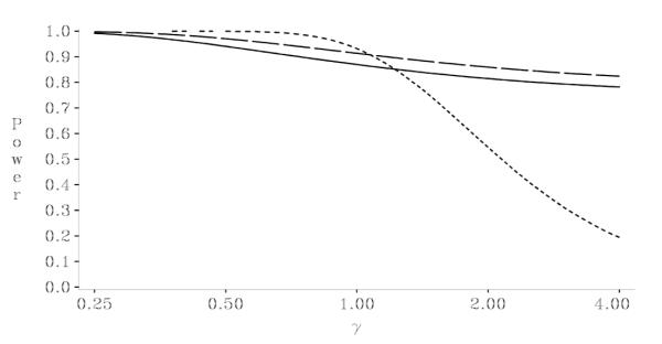
Plot of power as a function of $\gamma ={\sigma }^2∕{\sigma }_0^2$ for CLAHE example with α_t = 0.0011, P_t = 0.90, θ_* = 0.10, ${\sigma }_0^2$ = 0.0065, n₁ = 10, and n₀ 20, for: (a) Fixed sample design n₀ = 20: dotted line; (b) IP unadjusted = with test with n_+,min = 10 and n_+,max = ∞: dashed line; (c) IP bounding test with n_+,min = 10 and n_+,max = ∞: solid line

The luxury of fast calculations becomes a necessity when producing plots such as Figs. 1 and 2 to examine ranges of study designs. The speed of the new algorithms allows visualizing the tradeoffs among a variety of internal pilot designs. Generating the entire set of Type I error rate values for the unadjusted and bounding tests shown in Fig. 1 took approximately 5 and 20 s, respectively. In contrast, we estimate that the old algorithm, if it always converged, would take 10–20 min for each curve.

4. Conclusions

The new and much simpler density and cdf open new avenues for determining previously unknown exact and approximate analytic properties of internal pilot designs. Notable improvements in computing stability, speed, and accuracy illustrate the point emphatically: The bounding test becomes practical and convenient even in the small sample studies where it has the most value. The new algorithms are available in GLUMIP version 2.0, free SAS/IML® code available at www.soph.uab.edu/coffey.

The improved speed also allows quickly plotting power and expected sample size over wide ranges of design parameters. The ability to produce such plots in a timely manner has many advantages. For example, there is an obvious trade-off between choosing a large enough value of n₁ to ensure a reliable estimate of σ² and choosing the smallest possible value of n₁ such that modifications to sample size, and any corresponding logistical changes to the on-going study, can be implemented as early as possible. Examining plots of power over a wide range of design parameters can be used to determine the smallest value of n₁ retaining the desired benefits of an internal pilot.

As with all of our previous work, the new results apply to any general linear model with fixed predictors and Gaussian errors, and therefore include the t-test as a special case. The properties of internal pilot designs with repeated measures or other correlated outcomes have received only limited attention. Our current research focuses on extending the results to internal pilot designs with repeated measures and exploring additional improvements to the bounding test.

References

- Coffey CS, Muller KE. Exact test size and power of a Gaussian error linear model for an internal pilot study. Statist. Med. 1999;18:1199–1214. doi: 10.1002/(sici)1097-0258(19990530)18:10<1199::aid-sim124>3.0.co;2-0. [DOI] [PubMed] [Google Scholar]
- Coffey CS, Muller KE. Properties of doubly-truncated gamma variables. Commun. Statist. Theor. Meth. 2000a;29:851–857. doi: 10.1080/03610920008832519. [DOI] [PMC free article] [PubMed] [Google Scholar]
- Coffey CS, Muller KE. Some distributions and their implications for an internal pilot study with a univariate linear model. Commun. Statist. Theor. Meth. 2000b;29:2677–2691. doi: 10.1080/03610920008832631. [DOI] [PMC free article] [PubMed] [Google Scholar]
- Coffey CS, Muller KE. Controlling test size while gaining the benefits of an internal pilot design. Biometrics. 2001;57:625–631. doi: 10.1111/j.0006-341x.2001.00625.x. [DOI] [PubMed] [Google Scholar]
- Coffey CS, Muller KE. Properties of internal pilots with the univariate approach to repeated measures. Statist. Med. 2003;22:2469–2485. doi: 10.1002/sim.1466. [DOI] [PubMed] [Google Scholar]
- Davies RB. The distribution of a linear combination of 2 random variables. Appl. Statist. 1980;29:323–333. [Google Scholar]
- Friede T, Kieser M. Sample size recalculation in internal pilot study designs: a review. Biometrical J. 2006;4:537–555. doi: 10.1002/bimj.200510238. [DOI] [PubMed] [Google Scholar]
- Glueck DH, Muller KE. On the expected values of sequences of functions. Commun. Statist. Theor. Meth. 2001;30:363–369. doi: 10.1081/STA-100002037. [DOI] [PMC free article] [PubMed] [Google Scholar]
- Gould A, Shih W. Sample size re-estimation without unblinding for normally distributed outcomes with unknown variance. Commun. Statist. Theor. Meth. 1992;21:2833–2853. [Google Scholar]
- ICH Guideline E9 . International Conference on Harmonisation of Technical Requirements for Registration of Pharmaceuticals for Human Use. EMEA; London: 1998. ICH Topic E9: Statistical principles for clinical trials. ICH Technical Coordination. [Google Scholar]
- Jennison C, Turnbull BW. Group Sequential Methods with Applications to Clinical Trials. Chapman & Hall/CRC; Boca Raton, FL: 2000. [Google Scholar]
- Johnson NL, Kotz S, Balakrishnan N. Continuous Univariate Distributions - 1. 2nd ed Wiley; New York: 1994. [Google Scholar]
- Johnson NL, Kotz S, Balakrishnan N. Continuous Univariate Distributions - 2. 2nd ed Wiley; New York: 1995. [Google Scholar]
- Kiefer J. Sequential minimax search for a maximum. Proc. Amer. Mathemat. Soc. 1953;4:502–506. [Google Scholar]
- Kieser M, Friede T. Recalculating the sample size in internal pilot study designs with control of the type I error rate. Statist. Med. 2000;19:901–911. doi: 10.1002/(sici)1097-0258(20000415)19:7<901::aid-sim405>3.0.co;2-l. [DOI] [PubMed] [Google Scholar]
- Kieser M, Friede T. Simple procedures for blinded sample size adjustment that do not affect the type I error rate. Statist. Med. 2003;22:3571–3581. doi: 10.1002/sim.1585. [DOI] [PubMed] [Google Scholar]
- Miller F. Variance estimation in clinical studies with interim sample size reestimation. Biometrics. 2005;61:355–361. doi: 10.1111/j.1541-0420.2005.00315.x. [DOI] [PubMed] [Google Scholar]
- Pisano ED, Zong S, Hemminger BM, DeLuca M, Johnston RE, Muller KE, Brauening MP, Pizer SM. Contrast limited adaptive histogram equalization image processing to improve the detection of simulated speculations in dense mammograms. J. Digital Imaging. 1998;11:193–200. doi: 10.1007/BF03178082. [DOI] [PMC free article] [PubMed] [Google Scholar]
- Pizer SM, Zimmerman JB, Staab EV. Adaptive gray level assignment in CT scan display. J. Comput. Assisted Tomography. 1984;8:300–305. [PubMed] [Google Scholar]
- Proschan MA. Two-stage sample size re-estimation based on a nuisance parameter: a review. J. Biopharmaceutical Statist. 2005;15:559–574. doi: 10.1081/BIP-200062852. [DOI] [PubMed] [Google Scholar]
- Proschan MA, Wittes J. An improved double sampling procedure based on the variance. Biometrics. 2000;56:1183–1187. doi: 10.1111/j.0006-341x.2000.01183.x. [DOI] [PubMed] [Google Scholar]
- SAS Institute . SAS/IML® 9.1 User’s Guide, Volumes 1 and 2. SAS Institute; Cary, NC: 2004. [Google Scholar]
- Stein C. A two-sample test for a linear hypothesis whose power is independent of the variance. Ann. Mathemat. Statist. 1945;16:43–58. [Google Scholar]
- Wittes J, Brittain E. The role of internal pilot studies in increasing the efficiency of clinical trials. Statist. Med. 1990;9:65–72. doi: 10.1002/sim.4780090113. [DOI] [PubMed] [Google Scholar]
- Zucker DM, Wittes JT, Schabenberger O, Brittain E. Internal pilot studies II: comparison of various procedures. Statist. Med. 1999;18:3493–3509. doi: 10.1002/(sici)1097-0258(19991230)18:24<3493::aid-sim302>3.0.co;2-2. [DOI] [PubMed] [Google Scholar]