Automatic protein structure solution from weak X-ray data

Abstract

Determining new protein structures from X-ray diffraction data at low resolution or with a weak anomalous signal is a difficult and often an impossible task. Here we propose a multivariate algorithm that simultaneously combines the structure determination steps. In tests on over 140 real data sets from the protein data bank, we show that this combined approach can automatically build models where current algorithms fail, including an anisotropically diffracting 3.88 Å RNA polymerase II data set. The method seamlessly automates the process, is ideal for non-specialists and provides a mathematical framework for successfully combining various sources of information in image processing.

X-ray crystallography is a routine technique used to solve protein structures, but is often limited by weak anomalous scattering signals and low-resolution data. Here the authors develop a synergistic algorithm to significantly increase the success rate of structure solution when the signal is weak.

X-ray diffraction of macromolecular crystals does not provide a direct image of a molecule. The macromolecule’s electron density can be computationally constructed by exploiting the anomalous signal from heavy atoms, such as seleniums incorporated into a molecule of unknown fold. For data sets with a strong anomalous signal diffracting to resolutions better than 3 Å, current computational methods can usually automatically build an atomic model. Yet, determining crystal structures of large macromolecular assemblies or membrane proteins that tend to diffract to lower resolutions is difficult and involves manually iterating over the different steps in the structure solution process1 and still may not lead to an interpretable electron density map. Even at higher resolutions, diffraction data containing a weak anomalous signal can elude current computational methods and may require more data from other crystals2. Here we propose a new method that combines the traditional structure solution steps to push the limits of computational techniques.

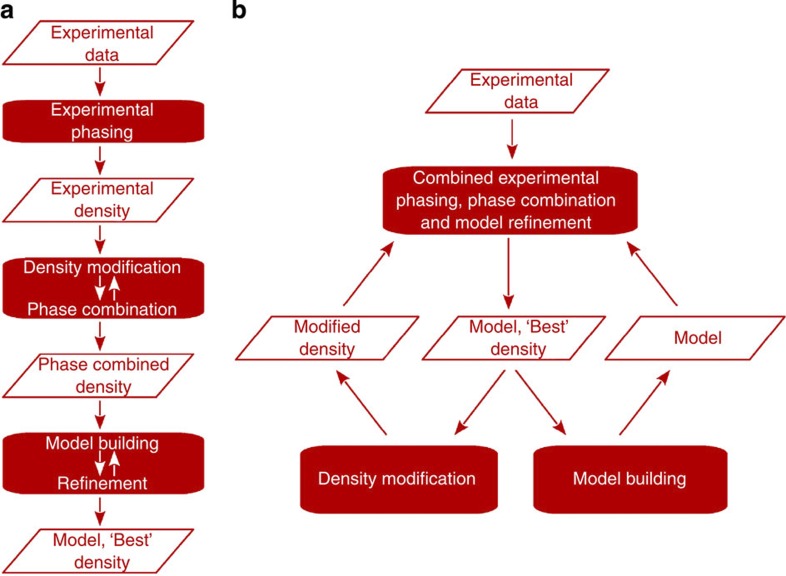
Currently, the process of solving a macromolecular crystal structure of unknown fold from X-ray data consists of distinct steps (Fig. 1a). In experimental phasing, crystallographic phase estimates are calculated by exploiting the signal from an anomalous substructure. An initial experimental electron density is constructed from these phase estimates and the X-ray data. Next, expected features of macromolecular electron density, such as the flatness of solvent regions, are imposed on the experimental electron density to improve its quality. This density-modified map is typically combined with the initial experimental density map in phase combination. Finally, the resulting electron density is used to iteratively build and refine a model of the macromolecule.

Figure 1. The current and new combined approach for structure solution.

(a) Currently, when solving a structure using anomalous scattering, the steps of experimental phasing, density modification with phase combination and model building with refinement are performed separately. (b) Unlike the traditional stepwise approach, the combined function simultaneously uses the information from density modification, model building and from the data to provide the best estimate of the electron density.

After the experimental density is constructed, information about the unknown phase and its accuracy is often ignored or approximated, and statically propagated to the steps of phase combination and model refinement via Hendrickson–Lattman coefficients3. We have previously demonstrated that using the experimental data and anomalous substructure directly in phase combination4 and model refinement5 via step-specific multivariate distributions can improve the individual steps.

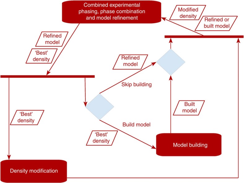
Here we present a novel combined multivariate probability function (Equation (2), see Methods section) that directly considers phase information from the experimentally collected X-ray data, and simultaneously combines it with the information from density modification and model building into a single unified process (Fig. 1b). The unified process consists of iterative minimization of the minus log-likelihood of the new combined probability distribution in reciprocal space, followed by current density modification and model-building procedures in crystal space. Thus, the structure solution process no longer relies on successive stepwise approximations of the experimental data. The full power of the new method is obtained by simultaneously considering the anomalous substructure, density-modified electron density map and partial protein model. If only the substructure is available, the new combined function elegantly reduces to the previously described experimental phasing function (Equation (3)). Similarly, when only the substructure and electron density are available, the combined function simplifies to the step-specific phase combination function. After a partial protein model has been built, the full combined probability distribution is used and all the information is exploited simultaneously. Results from our large collection of real data sets, described below, show that the best performance and efficiency of the new algorithm can be achieved by skipping the model-building step for some iterations (Fig. 2); currently, model building is first performed after 20 iterations and then repeated every eighth iteration. The total number of iterations is chosen automatically by the algorithm; more iterations are run for weaker signals.

Figure 2. Detailed diagram for the combined algorithm.

An expanded UML flowchart of the combined algorithm, which includes decision making (blue diamonds) to skip the model building.

Current automated structure solution systems use a stepwise approach (Fig. 1a) for structure solution, but can use different programmes or parameters for experimental phasing, density modification or model building. To objectively assess the new algorithm’s (Fig. 1b) power in a controlled fashion, we compare it against the stepwise algorithm using the same programmes and parameters. For both approaches, real-space density modification is performed in PARROT6 (version 1.0.2) and automated model building is performed in BUCCANEER7 (version 1.5.2). The new combined function, implemented in REFMAC8, simultaneously uses the information from real-space density modification and model building, whereas the current approach uses this information separately in stepwise phase combination and model refinement functions, also implemented in REFMAC. The automated structure solution package CRANK9 (version 2.0.0) is used to link these programmes for both approaches in this test. To assess the performance of the combined structure solution approach against another automated package, we also compare the new method against the default, recursive, stepwise approach of PHENIX AutoSol10 (version 1.8.2-1309). We find that the new combined algorithm performs significantly better in both the controlled test and in comparison with PHENIX, and led to many models built automatically when the current approaches failed.

Results

Large-scale and controlled comparison

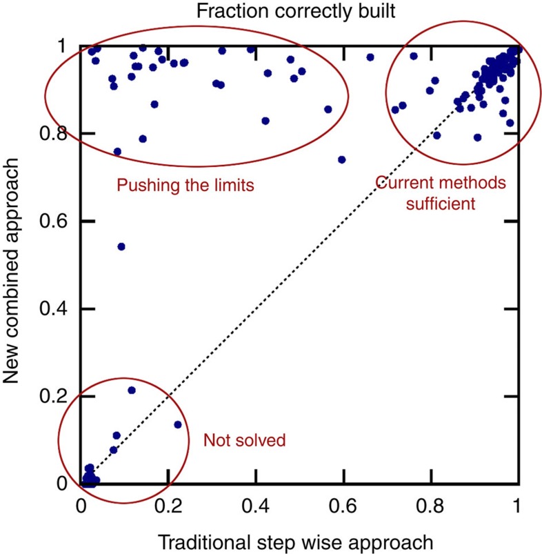
We test the performance and robustness of the new method for combined structure solution against the current stepwise approach on 147 single-wavelength anomalous diffraction (SAD) data sets spanning a wide range of resolutions from 0.94 to 3.88 Å and anomalous scatterers, including selenium, sulphur, chloride, iodide, bromide, calcium and zinc. Figure 3 compares the fraction of the 147 models automatically built within 1 Å of the deposited structure by the combined method on the y axis and the stepwise approach on the x axis, both implemented in CRANK. The cluster of points in the lower left corner of the plot represents the data sets where no model can be built, usually caused by the inability to find the heavy atom substructure. The data sets providing 85–100% complete models for both methods are depicted in the upper right corner. Finally, the ‘Pushing the limits’ cluster shows the numerous data sets for which partial or no model was built using the current stepwise method, but near complete models with the new combined method.

Figure 3. Comparison of CRANK's stepwise and combined approach.

The fraction of model correctly built by the CRANK's stepwise approach compared with the new multivariate combined method on 147 data sets. Each data set is represented by a circle. The y axis plots the fraction of model correctly built using the combined algorithm, whereas the x axis shows the performance of the stepwise traditional algorithm. The further a circle lies above the dotted diagonal line, the greater the improvement the new approach provides.

For all data sets, the average fraction of model correctly built increases from 60% to 74%. If we exclude the data sets built to at least 85% completeness by the stepwise method and data sets where the heavy atom substructure could not be found, 45 data sets remain with 28% of the model correctly built on average by the stepwise approach and 77% by the combined algorithm.

Large-scale comparison with PHENIX

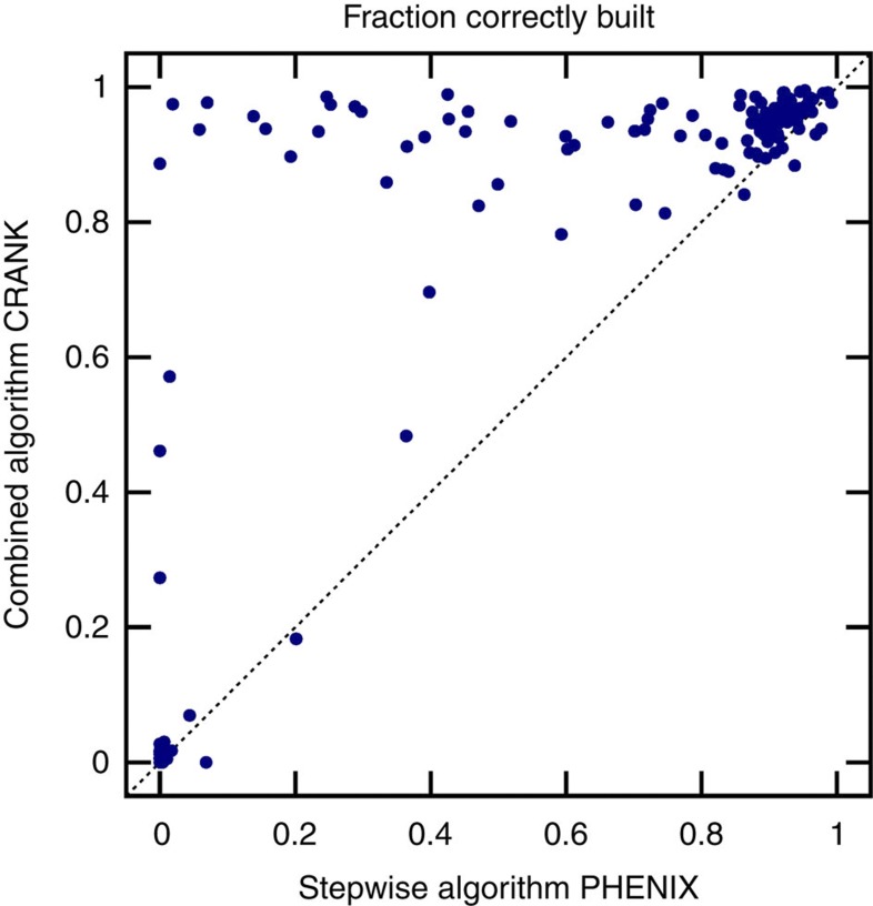
Figure 4 shows the fraction of the 147 models automatically built to within 1 Å of the deposited structure by the combined method and by the PHENIX AutoSol software. The results are similar to that of Fig. 3, showing many data sets significantly above the diagonal line for which no or a partial model is built using PHENIX, but nearly complete models with the combined method. Unlike in the controlled comparison of the stepwise and the combined algorithm shown in Fig. 3, we cannot draw direct conclusions about the performance of these algorithms, as although PHENIX also uses a stepwise approach it employs different programmes and parameters than CRANK. We can only conclude that with the default settings, more structures are built automatically with the combined approach in CRANK than with PHENIX for the random sample of 147 data sets: the average fraction correctly built increases from 59% to 74%.

Figure 4. Comparison of PHENIX and CRANK’s combined approach.

The fraction of model correctly built by PHENIX compared with the new multivariate combined method on 147 data sets. Each data set is represented by a circle. The y axis plots the fraction of model correctly built using the combined algorithm, whereas the x axis shows the performance of PHENIX. The further a circle lies above the dotted diagonal line, the greater the improvement the new approach provides.

RNA polymerase II data set (3.88 Å)

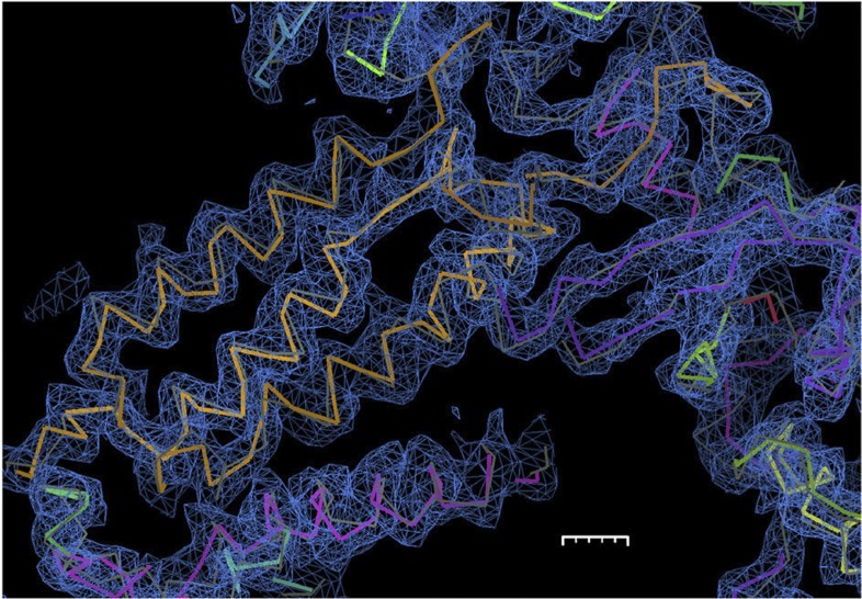
The performance of the new method at low resolution can be demonstrated on the 12-subunit RNA polymerase II SAD data set diffracting anisotropically to 3.88 Å (ref. 11) and containing 3,950 residues in the asymmetric unit. The authors could neither automatically nor manually build the structure from the SAD data set collected: structure solution was performed by a combination of multicrystal, multiple wavelength anomalous diffraction phasing from five crystals, molecular replacement from a partial model and manual iterative model building and refinement. The combined method results in automatic building of a majority of the protein backbone solely from the anomalous signal of eight intrinsic zinc atoms and the single SAD data set. The quality of the automatically built structure is evident from the R-free value12 of 37.6%. Figure 5 shows the agreement between the final and automatically built model, and the resulting electron density for a part of the RNA polymerase II molecule. 67% of the Cα positions were traced to 2 Å precision, 82%, to 2.5 Å precision, and 9% were placed incorrectly (see the Methods section for the definition we use to assess model-building quality that also requires a neighbouring Cα atom to be correctly placed).

Figure 5. RNA polymerase II electron density.

Electron density of a portion of the 3.88 Å RNA polymerase II structure automatically built by the new combined approach contoured at 2.1σ. The final Cα trace is shown in grey, whereas the automatically built model is multicoloured. This figure was made with COOT20. The length of the scale bar is 5 Å with minor ticks at 1 Å.

RNA polymerase clamp domain–Spt4/5 data set (3.3 Å)

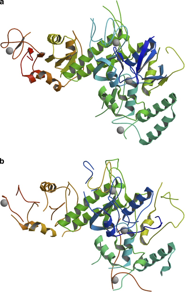
An RNA polymerase clamp domain–Spt4/5 complex13 was built manually from a partial molecular replacement model using a 3.3 Å SAD data set containing an anomalous signal from intrinsic zinc atoms. The authors could not get an interpretable electron density map from the anomalous signal alone. However, when using the combined algorithm, 77% of the deposited model backbone residues were automatically correctly built to the 2-Å criteria. Figure 6a,b show the deposited and automatically built structure, respectively. Table 1 shows model refinement and building statistics for these two low-resolution data sets.

Figure 6. Deposited and automatically built clamp domain–Spt4/5 models.

(a) The final, deposited structure of the related RNA polymerase clamp domain in complex with Spt4/5. (b) The automatically built structure using the combined method of the related RNA polymerase clamp domain in complex with Spt4/5. Fig. 6a,b were made with MOLSCRIPT21.

Table 1. Model-building statistics for the highlighted data sets.

	Resolution (Å)	Map correlation* after phasing	Map correlation* after structure solution	R-free	Model correctly built (%)
RNA polymerase	3.88	0.176	0.639	0.376	67
Clamp domain–Spt4/5	3.3	0.103	0.754	0.363	77

^*Correlations or fraction of model built were calculated using the structure deposited in the Protein Data Bank.

Discussion

The presented results demonstrate that the current limits of X-ray crystallography can be significantly extended by the synergistic effect of simultaneously combining the steps. Although the use of the combined method does not improve the automated structure solution if a substructure could not be found or if a nearly complete structure can be built by the current methods, its use substantially improves the automated model building limited by a weak anomalous signal or a low resolution.

The mathematical framework presented here is certainly not limited to X-ray crystallography, but can be applied to other techniques such as cryo-electron microscopy where a related maximum likelihood analysis14 can be generalized and combined with, for example, model building15, while considering the observed experimental data/images directly. Both CRANK and REFMAC are open-source packages and these latest developments will be available from CCP4 ( http://www.ccp4.ac.uk/).

Methods

Testing methodology

The new function and algorithm have been tested on 147 real SAD data sets mainly composed of the same data sets used previously4: all data sets are listed in Supplementary Table S1. The diffraction data, the sequence of the protein monomer, the f′ and f′′ values for the substructure atoms and the substructure as determined by SHELXC and SHELXD16, or AFRO9 and CRUNCH2 (ref. 17), were input to PHENIX and to CRANK’s stepwise and combined pipelines. All three approaches were run with default settings.

The combined algorithm and the PHENIX AutoSol software automatically choose the number of model-building cycles (the current defaults for the CRANK implementation of the combined algorithm are a minimum of 5 and a maximum of 50 building cycles). In CRANK’s stepwise approach, the density-modified map from PARROT is input to model building by BUCCANEER, which is iterated 50 times with refinement by the multivariate SAD function5 in REFMAC (Equaton (3)). If the fraction of model built after the first 5 building cycles was higher than after 50 cycles, it was used for comparison with the combined algorithm’s results, otherwise the fraction built after 50 cycles was used.

The quality of the protein models built is expressed as a fraction of the Protein Data Bank-deposited model backbone ‘correctly built’. In the massive testing on 147 data sets, a residue is considered correctly built if its Cα position is at most 1 Å distant from a deposited model Cα (Cα-deposited) position. For the highlighted low-resolution cases, a 2-Å criteria18 is used, as 1 Å is a minimal estimate of the coordinate uncertainty at 4 Å resolution19. However, we add an additional requirement that a neighbouring Cα position must be at most 2 Å distant from a neighbour of Cα deposited for the residue to be considered correctly built. A residue is considered incorrectly built if it is >2.5 Å distant from the nearest Cα-deposited position. Furthermore, a residue is also considered incorrectly built if it is <2.5 Å distant from the Cα deposited, but none of its neighbouring Cα positions are closer than 2.5 Å from a neighbour of Cα deposited.

The combined likelihood function

To apply a maximum likelihood analysis that combines the information from the different steps in macromolecular X-ray crystallography and incorporates the observed experimental diffraction data directly, the multivariate probability distribution of the observed SAD structure factor amplitudes (), given the partial (anomalous and/or non-anomalous) calculated structure factors () and density modification structure factors (F_DM=F_DMexp(iα_DM)) is required. Here the subscripts O,C,DM denote observed, partial anomalous and/or non-anomalous calculated, and density modification structure factors, respectively, and the + and − superscripts denote the Friedel pairs. To derive the above distribution, the starting point is the multivariate distribution of structure factors:

The distribution for equation (1) is well approximated by a complex multivariate Gaussian distribution via the Central Limit Theorem. After transforming the multivariate complex Gaussian to polar coordinates and integrating out the unknown ‘observed’ structure factor phases, the required distribution is obtained:

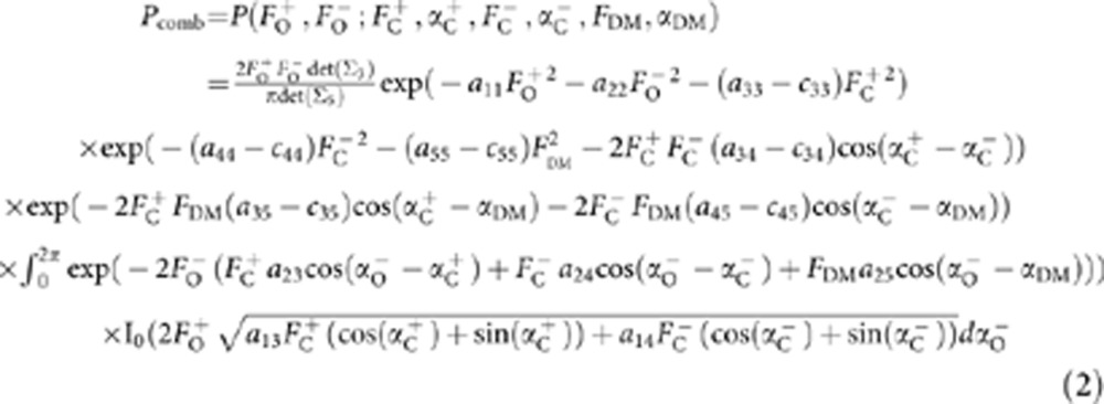In equation (2), a_ij is the ijth element of the inverse of the full 5 × 5 covariance matrix Σ₅ and c_ij is the ijth element of the model 3 × 3 (Σ₃) submatrix of Σ₅. If the density modification structure factor, F_DM, is not available, the equation reduces to the previously described multivariate function for SAD-based model refinement function5:

In equation (3), a_ij is the ijth element of the inverse of the 4 × 4 covariance matrix Σ₄ that is a submatrix of Σ₅ and c_ij is the ijth element of the model 2 × 2 (Σ₂) submatrix of Σ₄. If the partial structure factors consist only or mainly of contributions from anomalous atoms, such as those found in substructure detection, equation (3) reduces into the previously described function for multivariate heavy atom refinement and phasing, only differing by the covariance matrix Σ₄ definition. Similarly, if only density modification structure factors and anomalous atoms are available for calculation of , equation (2) reduces to the previously described multivariate phase combination function4, differing by the covariance matrix Σ₅ definition. These special cases have all been implemented in the programme REFMAC.

Author contributions

P.S. and N.S.P. designed the research, analysed the results and wrote the manuscript. P.S. wrote the computer source code and ran the test cases.

Additional information

How to cite this article: Skubák, P. & Pannu, N. S. Automatic protein structure solution from weak X-ray data. Nat. Commun. 4:2777 doi: 10.1038/ncomms3777 (2013).

Supplementary Material

Supplementary Table

Supplementary Table S1

References

- Schroder G., Levitt M. & Brunger A. T. Super-resolution biomolecular crystallography with low-resolution data. Nature 464, 1218–1222 (2010). [DOI] [PMC free article] [PubMed] [Google Scholar]
- Liu Q. et al. Structures from anomalous diffraction data of native biological macromolecules. Science 336, 1033–1037 (2012). [DOI] [PMC free article] [PubMed] [Google Scholar]
- Hendrickson W. A. & Lattman E. E. Representation of phase probability distributions for simplified combination of independent phase information. Acta Cryst. B26, 136–143 (1970). [Google Scholar]
- Skubak P., Waterreus W. J. & Pannu N. S. Multivariate phase combination improves automated crystallographic model building. Acta Cryst. D66, 783–788 (2010). [DOI] [PubMed] [Google Scholar]
- Skubak P., Murshudov G. N. & Pannu N. S. Direct incorporation of experimental phase information in model refinement. Acta Cryst. D60, 2196–2201 (2004). [DOI] [PubMed] [Google Scholar]
- Cowtan K. Recent developments in classical density modification. Acta Cryst. D66, 470–478 (2010). [DOI] [PMC free article] [PubMed] [Google Scholar]
- Cowtan K. The Buccaneer software for automated model building. 1. Tracing protein chains. Acta Cryst. D62, 1002–1011 (2006). [DOI] [PubMed] [Google Scholar]
- Murshudov G. N. et al. REFMAC5 for the refinement of macromolecular crystal structures. Acta Cryst. D67, 355–367 (2011). [DOI] [PMC free article] [PubMed] [Google Scholar]
- Pannu N. S. et al. Recent advances in the CRANK software suite for experimental phasing. Acta Cryst. D67, 331–337 (2011). [DOI] [PMC free article] [PubMed] [Google Scholar]
- Adams P. D. et al. PHENIX: a comprehensive Python-based system for macromolecular structure solution. Acta Cryst. D66, 213–221 (2010). [DOI] [PMC free article] [PubMed] [Google Scholar]
- Meyer P. A., Ye P., Zhang M., Suh M. H. & Fu J. Phasing RNA polymerase II using intrinsically bound Zn atoms: an updated structural model. Structure 14, 973–982 (2006). [DOI] [PubMed] [Google Scholar]
- Brunger A. T. The free R value: a novel statistical quantity for assessing the accuracy of crystal structures. Nature 355, 472–475 (1992). [DOI] [PubMed] [Google Scholar]
- Martinez-Rucobo F. W., Sainsbury S., Cheung A. C. M. & Cramer P. Achitecture of the RNA Polymerase-Spt4/5 complex and basis of universal transcription processivity. EMBO J. 30, 1302–1310 (2011). [DOI] [PMC free article] [PubMed] [Google Scholar]
- Sigworth F. J., Doerschuk P. C., Carazo J. M. & Scheres S. H. An introduction to maximum likelihood methods in cryo-EM. Methods Enzymol. 482, 263–294 (2010). [DOI] [PMC free article] [PubMed] [Google Scholar]
- Liu H. et al. Atomic structure of human adenovirus by cryo-EM reveals interactions among protein networks. Science 329, 1038–1043 (2010). [DOI] [PMC free article] [PubMed] [Google Scholar]
- Sheldrick G. M. A short history of SHELX. Acta Cryst. A64, 112–122 (2008). [DOI] [PubMed] [Google Scholar]
- de Graaff R. A. G., Hilge M., van der Plas J. L. & Abrahams J. P. Matrix methods for solving protein substructures of chlorine and sulfur from anomalous data. Acta Cryst. D57, 1857–1862 (2001). [DOI] [PubMed] [Google Scholar]
- Brunger A. T., Adams P. D., Fromme P., Fromme R., Levitt M. & Schroeder G. F. Improving the accuracy of macromolecular structure refinement at 7A resolution. Structure 20, 957–966 (2012). [DOI] [PMC free article] [PubMed] [Google Scholar]
- Brunger A. T. Free R value: cross-validation in crystallography. Methods Enzymol. 277, 366–396 (1997). [DOI] [PubMed] [Google Scholar]
- Emsley P., Lohkamp B., Scott W. G. & Cowtan K. Features and development of Coot. Acta Cryst. D66, 486–501 (2008). [DOI] [PMC free article] [PubMed] [Google Scholar]
- Kraulis P. J. MOLSCRIPT: a program to produce both detailed and schematic plots of protein structures. J. Appl. Cryst. 24, 946–950 (1991). [Google Scholar]
Associated Data
This section collects any data citations, data availability statements, or supplementary materials included in this article.
Supplementary Materials