Optimal indolence: a normative microscopic approach to work and leisure

Abstract

Dividing limited time between work and leisure when both have their attractions is a common everyday decision. We provide a normative control-theoretic treatment of this decision that bridges economic and psychological accounts. We show how our framework applies to free-operant behavioural experiments in which subjects are required to work (depressing a lever) for sufficient total time (called the price) to receive a reward. When the microscopic benefit-of-leisure increases nonlinearly with duration, the model generates behaviour that qualitatively matches various microfeatures of subjects’ choices, including the distribution of leisure bout durations as a function of the pay-off. We relate our model to traditional accounts by deriving macroscopic, molar, quantities from microscopic choices.

1. Introduction

What to do, when to do it and how long to do it for are fundamental questions for behaviour. Different options across these dimensions of choice yield different costs and benefits, making for a rich, complex, optimization problem.

One common decision is between working (performing an employer-defined task) and engaging in leisure (activities pursued for oneself). Working leads to external rewards, such as food and money; whereas leisure is supposed to be intrinsically beneficial (otherwise, one would not want to engage in it). As these activities are usually mutually exclusive, subjects must decide how to allocate time to each. Note that work need not be physically or cognitively demanding, but consumes time; equally leisure need not be limited to rest and may present physical and/or mental demands.

This decision has been studied by economists [1–5], behavioural psychologists [6–16], ethologists [17] and neuroscientists [18–24]. Tasks involving free-operant behaviour are particularly revealing, because subjects can choose what, when and how, minimally encumbered by direct experimenter intervention. We consider the cumulative handling time (CHT) schedule brain stimulation reward (BSR) paradigm of Shizgal and co-workers [20,21], in which animals have to invest quantifiable work to get rewards that are psychophysically stationary and repeatable.

Most previous investigations of time allocation (TA) have focused on molar or macroscopic characterizations of behaviour [1,2,4,10,18,21–23,25–31], capturing the average times allocated to work or leisure. Here, we characterize the detailed temporal topography of choice, i.e. the fine-scale molecular or microscopic structure of allocation [32–37], that is lost in molar averages (figure 1c). We build an approximately normative, reinforcement-learning, account, in which microscopic choices approximately maximize net benefit. Our central intent is to understand the qualitative structure of the molecular behaviour of subjects, providing an account that can generalize to many experimental paradigms. Therefore, although we apply the model to a set of CHT experiments in rats it is the next stage of the programme to fit this behaviour quantitatively in detail.

Figure 1.

Task and key features of the data. (a) CHT task. Grey bars denote work (depressing a lever), white gaps show leisure. The subject must accumulate work up to a total period of time called the price (P) in order to obtain a single reward (black dot) of subjective RI. The trial duration is 25×price (plus 2 s each time the price is attained, during which the lever is retracted so it cannot work; not shown). The RI and price are held fixed within a trial. (b) Molar TA functions of a typical subject as a function of RI and price. Red/grey curves: effect of RI, for a fixed short price; blue/dark grey curves: effect of price, for a fixed high RI; green/light grey curves: joint effect of RI and price. (c) A molecular analysis may reveal different microstructures of working and engaging in leisure. The three rows show three different hypothetical trials. All three microstructures have the same molar TA, but are clearly distinguishable. (d) Molecular ethogram showing the detailed temporal topography of working and engaging in leisure for the subject in (b). Upper, middle and lower panels show low, medium and high pay-offs, respectively, for a fixed, short price. Following previous reports using rat subjects, releases shorter than 1 s are considered part of the previous work bout (as subjects remain at the lever during this period). Graphically, this makes some work bouts appear longer than the others. The subject mostly pre-commits to working continuously for the entire price duration. When the pay-off is high, the subject works almost continuously for the entire trial, engaging in very short leisure bouts inbetween work bouts. When the pay-off is low, the subject engages in a long leisure bout after receiving a reward. This leisure bout is potentially longer than the trial, whence it would be censored. The part of a trial before the reward, price and probability of reward delivery are certainly known is coloured pink/dark and not considered further. Data collected by Y.-A.B. and R.S. and initially reported in [38]. (Online version in colour.)

Having introduced previous approaches, we describe an example task and experiments (§2), key molecular features of the data from those (§3), our novel normative, microscopic approach (§4) and how it captures these key features (§5).

2. Task and experiment

As an example paradigm employed in rodents, consider a CHT task [20,21] in which subjects choose between working—the facile task of holding down a light lever—and engaging in leisure, i.e. resting, grooming, exploring, etc. (figure 1a). A BSR [38] is given after the subject has accumulated work for an experimenter-defined total time-period called the price (P; see table 1 for a description of all symbols). BSR does not suffer satiation and allows precise, psychophysically stable data to be collected over many months. We show data initially reported in [39] (and subsequently in [40,41]).

Table 1.

List of symbols.

symbol	meaning
1/λ	mean of exponential effective prior probability density for leisure time
α ∈ [0,1]	weight on linear component of microscopic benefit-of-leisure
β ∈ [0,∞)	inverse temperature or degree of stochasticity–determinism parameter
CHT	cumulative handling time
CL(·)	microscopic benefit-of-leisure
	maximum of sigmoidal microscopic benefit-of-leisure
	shift of sigmoidal microscopic benefit-of-leisure
δ(·)	delta/indicator function
	expected value with respect to policy π
KL	slope of linear microscopic benefit-of-leisure
L	leisure
μa(τa)	effective prior probability density of choosing duration τa
P	price
	policy or choice rule: probability of choosing action a, for duration τa from state s
post	post-reward
pre	pre-reward
	expected return or (differential) Q-value of taking action a, for duration τa from state s
ρ	reward rate
ρτa	opportunity cost of time for taking action a for duration τa
RI	(subjective) reward intensity
	pay-off
s	state
TA	time allocation
τL	duration of instrumental leisure
τPav	Pavlovian component of post-reward leisure
τW	duration of work
W	work
w ∈ [0, P)	amount of work time so far executed out of the price
V(s)	expected return or value of state s

The objective strength of the BSR is the frequency of electrical stimulation pulses applied to the medial forebrain bundle. This is assumed to have a subjective worth, or microscopic utility (to distinguish it from the macroscopic utility described in [18–23]) called the reward intensity (RI, in arbitrary units). The transformation from objective to subjective worth has been previously determined [42–47]. The ratio of the RI to the price is called the pay-off. Leisure is assumed to have an intrinsic subjective worth, although its utility remains to be quantified. Throughout a task trial, the objective strength of the reward and price are held fixed. The total time a subject could work per trial is 25 times the price (plus extra time for ‘consuming’ rewards) enabling at most 25 rewards to be harvested. A behaviourally observed work or leisure bout is defined as a temporally continuous act of working or engaging in leisure, respectively. Of course, contiguous short work or leisure bouts are externally indistinguishable from one long bout. Subjects are free to distribute leisure bouts in between individual work bouts.

Subjects face triads of trials: ‘leading’, ‘test’ then ‘trailing’ (electronic supplementary material, figure S1). Leading and trailing trials involve maximal and minimal reward intensities, respectively, and the shortest price (we use the qualifiers ‘short’, ‘long’, etc., to emphasize that the price is an experimenter determined time-period). We analyse the sandwiched test trials, which span a range of prices and reward intensities. Leading and trailing trials allow calibration, so subjects can stably assess RI and P on test trials. Subjects tend to be at leisure on trailing trials, limiting physical fatigue. Subjects repeatedly experience each test RI and price over many months, and so can readily appreciate them after minimal experience on a given trial without uncertainty.

3. Molar and molecular analyses of data

The key molar statistic is the TA, namely the proportion of the available time for working in a test trial that the subject spends pressing the lever. Figure 1b shows example TAs for a typical subject. TA increases with the RI and decreases with the price. Conversely, a molecular analysis, shown in the ethograms in (figure 1c,d), assesses the detailed temporal topography of choice, recording when, and for how long, each act of work or leisure occurred (after the first acquisition of the reward in the trial, i.e. after the ‘pink/dark grey’ lever presses in figure 1d). The TA can be derived from the molecular ethogram data, but not vice versa, because many different molecular patterns (figure 1c) share a single TA.

Qualitative characteristics of the molecular structure of the data (figure 1d) include: (i) at high pay-offs, subjects work almost continuously, engaging in little leisure inbetween work bouts; (ii) at low pay-offs, they engage in leisure all at once, in long bouts after working, rather than distributing the same amount of leisure time into multiple short leisure bouts; (iii) subjects work continuously for the entire price duration, as long as the price is not very long (as shown by an analysis conducted by Y.-A.B., to be published separately) and (iv) the duration of leisure bouts is variable.

4. Micro-semi-Markov decision process model

We consider whether key features of the data in figure 1d might arise from the subject's making stochastic optimal control choices, i.e. ones that at least approximately maximize the expected return arising from all benefits and costs over entire trials. Following [24], we formulate this computational problem using the reinforcement-learning framework of infinite horizon (Semi) Markov decision processes ((S)MDPs) [48,49] (figure 2a). Subjects not only choose which action a to take, i.e. to work (W) or engage in leisure (L), but also the duration of the action (τ_a). They pay an automatic opportunity cost of time: performing an action over a longer period denies the subject the opportunity to take other actions during that period, and thus extirpates any potential benefit from those actions.

Figure 2.

Model and leisure functions. (a) The infinite horizon micro-SMDP. States are characterized by whether they are pre- or post-reward. Subjects choose not only whether to work or to engage in leisure, but also for how long to do so. Pre-reward states are further defined by the amount of work time w that the subject has so far invested. At a pre-reward state [pre, w], the subject can choose to work (W) for a duration τ_W or engage in leisure (L) for a duration τ_L. Working for τ_W transitions the subject to a subsequent pre-reward state [pre, w+τ_W] if w+τ_W < P, and to the post-reward state if w+τ_W ≥ P. Engaging in leisure for τ_L transitions the subject to the same state. For working, only transitions to the post-reward state are rewarded, with reward intensity RI. Engaging in leisure for τ_L has a benefit C_L(τ_L). In the post-reward state, the subject is assumed already to have been at leisure for a time τ_Pav, which reflects Pavlovian conditioning to the lever. By choosing to engage in instrumental leisure for a duration τ_L, it gains a microscopic benefit-of-leisure C_L(τ_Pav+τ_L), and then returns to state [pre, 0] at the start of the cycle whence the process repeats. ((b)(i)): canonical microscopic benefit-of-leisure functions C_L(·); (ii): the net microscopic benefit-of-leisure per unit time spent in leisure. For simplicity, we considered linear C_L(·) (blue/dark grey), whose net benefit per unit time is constant, sigmoidal C_L(·) (red/grey), which is initially supralinear but eventually saturates, and so has a unimodal net benefit per unit time; and a weighted sum of these two (green/light grey). See the electronic supplementary material, equation (S-3) for details. (c) Time τ_Pav is the Pavlovian component of leisure, reflecting conditioning to the lever. It is decreasing with RI (here, inversely) and increasing with price (here sigmoidally), so that it decreases with pay-off. (Online version in colour.)

As trials are substantially extended, we assume that the subjects do not worry about the time the trial ends, and instead make choices that would (approximately) maximize their average summed microscopic utility per unit time [24]. Nevertheless, for comparison to the data, we still terminate each trial at 25× price, so actions can be censored by the end of the trial, preventing their completion.

4.1. Utility

The utility of the reward is RI. We assume that pressing the lever requires such minimal force that it does not incur any direct effort cost. We assume leisure to be intrinsically beneficial according to a function C_L(τ) of its duration (but formally independent of any other rewards or costs). The simplest such function is linear C_L(τ) = K_Lτ (figure 2b(i), blue/dark grey line), which would imply that the net utility of several short leisure bouts would be the same as a single bout of equal total length (figure 2b(ii), blue/dark grey line).

Alternatively, C_L(·) could be supralinear (figure 2b(i), red/grey curve). For this function, a single long leisure bout would be preferred to an equivalent time spent in several short bouts (figure 2b(ii), red/grey curve). If C_L(·) saturates, the rate of accrual of benefit-of-leisure dC_L(τ)/dτ will peak at an optimal bout duration. We represent this class of functions with a sigmoid, although many other nonlinearities are possible. Finally, to encompass both extremes, we consider a weighted sum of linear and sigmoid C_L(·), with the same maximal slope (figure 2b, green/light grey curve. Linear C_L(·) has weight α = 1, electronic supplementary material, equation (S-3)).

Evidence from related tasks [50,51] suggests that the leisure time will be subject to Pavlovian as well as instrumental influences [52–54]. Subjects exhibit high error rates and slow reaction times for trials with high net pay-offs, even when this is only detrimental. We formalize this with a leisure time as a sum of a mandatory Pavlovian contribution τ_Pav (in addition to the extra time for ‘consuming’ rewards), and an instrumental contribution τ_L, chosen, in the light of τ_Pav, to optimize the expected return. The Pavlovian component comprises a mandatory pause, which is curtailed by the subject's reengagement (conditioned-response) with the reward (unconditioned-stimulus)-predicting lever (conditioned-stimulus). As we shall discuss, we postulate a Pavlovian component to account for the detrimental leisure bouts at high pay-offs. We assume τ_Pav = f_Pav (RI, P) decreases with pay-off—i.e. increases with price and decreases with RI (figure 2c). The net microscopic benefit-of-leisure is then C_L(τ_L + τ_Pav) over a bout of total length τ_L + τ_Pav.

4.2. State space

The state in the model contains all the information required to make a decision. This comprises a binary component (‘pre’ or ‘post’), reporting whether or not the subject has just received a reward; and a real-valued component, indicating if not, how much work w ∈ [0, P) out of the price P has been performed. Alternatively, P–w is how far the subject is from the price.

4.3. Transitions

At state [pre, w], the subject can choose to work (W) for a duration τ_W or engage in leisure (L) for a duration τ_L. If it chooses the latter, it enjoys a benefit-of-leisure C_L(τ_L) for time τ_L, after which it returns to the same state. If the subject chooses to work up to a time that is less than the price, (i.e. w + τ_W < P), then its next state is 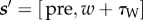. However, if w + τ_W ≥ P, the subject gains the work reward RI and transitions to the post-reward state , consuming time P–w. Although subjects can choose work durations τ_W that go beyond the price, they cannot physically work for longer than this time, because the lever is retracted as the reward is delivered.

In the post-reward state the subject can add instrumental leisure for time τ_L to the mandatory Pavlovian leisure τ_Pav discussed above. It receives utility C_L(τ_L+τ_Pav) over time τ_L+τ_Pav, and then transitions to state The cycle then repeats.

In all the cases, the subject's next state in the future depends on its current state s, the action a and the duration τ_a, but is independent of all other states, actions and durations in the past, making the model an SMDP. The model is molecular, as it generates the topography of lever depressing and releasing. It is microscopic as it commits to particular durations of performing actions. We therefore refer to it as a micro-SMDP. In the Discussion section, we consider an alternate, nanoscopic variant which makes choices at a finer timescale.

4.4. Policy evaluation

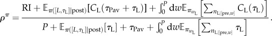
A (stochastic) policy π determines the probability of each choice of action and duration. It is assumed to be evaluated according to the average reward rate (see electronic supplementary material, equation (S-1)). In the SMDP, the state cycles between ‘pre-’ and ‘post-'reward. The average reward rate is the ratio of the expected total microscopic utility accumulated during a cycle to the expected total time that a cycle takes. The former comprises RI from the reward and the expected microscopic utilities of leisure; the latter includes the price P and the expected duration engaged in leisure.

The total average reward rate is

4.1

Here, π([L, τ_L]|post) and are the probabilities of engaging in instrumental leisure L for time τ_L in the post-reward and pre-reward state [pre, w], respectively; is the expectation over those probabilities. is the (random) number of times the subject engages in leisure in the pre-reward state [pre, w].

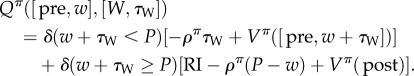
For state s = post, the action a = [L, τ_L] of engaging in leisure for time τ_L has differential value Q^π(post,[L, τ_L]) (see the electronic supplementary material, equation (S-2)) that includes three terms: (i) the microscopic utility of the leisure, C_L(τ_L+τ_Pav); (ii) opportunity cost –ρ^π(τ_L+τ_Pav) for the leisure time (the rate of which is determined by the overall average reward rate) and (iii) the long-run value V^π([pre, 0]) of the next state. The value of state s is defined as

averaging over the actions and durations that the policy π specifies at state s. Thus,

4.2

Note the clear distinction between the immediate microscopic benefit-of-leisure C_L (τ_L+τ_Pav) and the net benefit of leisure, given by the overall Q-value.

The value Q^π([pre, w], [L, τ_L]) of engaging in leisure for τ_L in the pre-reward state has the same form, but without the contribution of τ_Pav, and with a different subsequent state

4.3

Finally, the value Q^π([pre, w], [W, τ_W] of working for time τ_W in the pre-reward state has two components, depending on whether or not the accumulated work time w+τ_W is still less than the price (defined using a delta/indicator function as δ(w + τ_W < P)).

4.4

4.5. Policy

We assume the subject's policy π is stochastic, based on a softmax of the (differential) value of each choice, i.e. favouring actions and durations with greater expected returns. Random behavioural lapses make extremely long leisure or work bouts unlikely; we therefore consider a probability density μ_a(τ_a) of choosing duration τ_a (potentially depending on the action a), which is combined with the softmax like prior and likelihood (see the electronic supplementary material, text S1). We consider an alternative in the Discussion. For leisure bouts, we assume μ_L(τ_L) = λ exp(–λτ_L) is exponential with mean 1/λ = 10P. The prior μ_W(τ_W) for work bouts plays little role, provided its mean is not too short. This makes

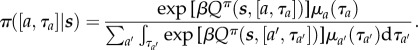4.5

Subjects will be more likely to choose the action with the greatest Q-value, but have a non-zero probability of choosing a suboptimal action. The parameter β ∈ [0, ∞) controls the degree of stochasticity in choices. Choices are completely random if β = 0, whereas β → ∞ signifies optimal choices. We use policy iteration [48,49] in order to compute policies that are self-consistent with their Q-values: these are the dynamic equilibria of policy iteration (see the electronic supplementary material, text S1). An alternative would be to compute optimal Q-values and then make stochastic choices based on them; however, this would lead to policies that are inconsistent with their Q-values. We shall show that stochastic, approximately optimal self-consistent choices lead to pre-commitment to working continuously for the entire price duration.

5. Micro-semi-Markov decision process policies

We first use the micro-SMDP to study the issue of stochasticity, then consider the three main regimes of behaviour evident in the data in figure 1d: when pay-offs are high (subjects work almost all the time), low (subjects never work) and medium (when they divide their time). Finally, we discuss the molar consequences of the molecular choices made by the SMDP. All throughout, RI and P are adopted from experimental data, while the parameters governing the benefit-of-leisure are the free parameters of interest.

5.1. Stochasticity

To illustrate the issues for the stochasticity of choice, we consider the case of a linear C_L(τ_L+τ_Pav) = K_L(τ_L+τ_Pav) and make two further simplifications: the subject does not engage in leisure in the pre-reward state (thus working for the whole price); and λ = 0, licensing arbitrarily long leisure durations. Then the Q-value of leisure is linear in τ_L, so the leisure duration distribution is exponential (see the electronic supplementary material, text S2). The expected reward rate and mean leisure duration can be derived analytically (see the electronic supplementary material, text S3).

As long as

5.1

Otherwise, if , then ρ^π → K_L (figure 3a(ii),b(ii)) and the subject would choose to engage in leisure for the entire trial as (figure 3a(i),b(i)).

Figure 3.

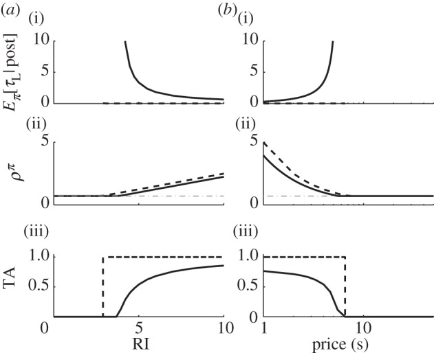
Effect of stochasticity. We use a linear microscopic benefit-of-leisure function (α = 1) to demonstrate the effect of stochasticity on: (i), mean instrumental leisure, post-reward; (ii), expected reward rate; (iii), TA as a function of (a) RI and (b) price. Solid and dashed black lines denote stochastic (β = 1) and deterministic, optimal (β → ∞) choices, respectively. Grey dash-dotted line in (ii) are ρ^π = K_L. TAs are step functions under a deterministic, optimal policy but smooth under a stochastic one. Price P = 4s in (a), while RI = 4.96 in (b).

Deterministically optimal behaviour requires β → ∞. In that case, provided RI > K_LP, the subject would not engage in leisure at all () but would work the entire trial (interspersed by only Pavlovian leisure τ_Pav) with optimal reward rate ρ* = (RI+K_Lτ_Pav)/(P+τ_Pav) (figure 3a(i),b(i) and a(ii),b(ii), respectively, dashed black lines). However, if RI < K_LP, then it would engage in leisure for the entire trial. Thus, TA functions would be step functions of the RI and price, as shown by the dashed black lines in figure 3a(iii),b(iii).

Of course, as is amply apparent in figure 1d, actual behaviour shows substantial variability, motivating stochastic choices, with β < ∞. As all the other quantities can be scaled, we set β = 1 without loss of generality. This leads to smoothly changing TA functions, expected leisure durations and reward rates, as shown by the solid lines in figure 3. We now return to the general case (λ ≠ 0, and leisure is possible in the pre-reward state).

5.2. High pay-offs

The pay-off is high when the RI is high or the price is short, or both. Subjects work as much as possible, making the reward rate in equation (4.1) ρ^π ≈ (RI+C_L(τ_Pav))/(P+τ_Pav). As τ_Pav is small for high pay-offs, ρ^π ≈ RI/P is just the pay-off of the trial. The opportunity cost of leisure time ρ^π(τ_L+τ_Pav) is then linear with a very steep slope (dash-dotted line in figure 4a(i)), which dominates C_L(τ_L+τ_Pav) (dashed line in figure 4a(i)), irrespective of which form it follows. The Q-value of engaging in leisure in the post-reward state then becomes the linear opportunity cost of leisure time, i.e. Q^π(post,[L, τ_L]) → –ρ^π(τ_L+τ_Pav) (solid bold line in figure 4a(i)).

Figure 4.

Q-values and policies for a high pay-off. ((a)(i)) and (ii) show Q-values and policies for engaging in instrumental leisure for time τ_L, respectively, in the post-reward state for three canonical C_L(·). In (i), solid bold curves show Q-values; coloured/grey dashed and dash-dotted lines show C_L(·) and the opportunity cost of time, respectively. Black dashed line is the linear component from the effective prior probability density for leisure time –λτ_L. Note the different y-axis scales. (b,d) Q-values and (c,e) policies for (b,c) engaging in leisure for time τ_L and (d,e) working for time τ_W in a pre-reward state [pre, w]. Light to dark colours shows increasing w, i.e. subject is furthest away from the price for light, and nearest to it for dark. (f) Probability of engaging in leisure for net time τ_L+τ_Pav in the post-reward state for sigmoid C_L(·) (α = 0). This is the same as the right in ((a)(ii)) but shifted by τ_Pav, RI = 4.96, price P = 4s. (Online version in colour.)

From equation (4.5), the probability density of engaging in instrumental leisure for time τ_L is π([L, τ_L] |post) ∝ exp[–(βρ^π + λ)τ_L]. This is an exponential distribution with very short mean (figure 4a(ii)). The net post-reward leisure bout, consisting of both Pavlovian and instrumental components has the same distribution, only shifted by τ_Pav, i.e. a lagged exponential distribution with mean (figure 4f).

The probability of choosing to engage in leisure in a pre-reward state (i.e. after the potential resumption of working) is correspondingly also extremely small. Furthermore, the steep opportunity cost of not working would make the distribution of any pre-reward leisure duration also be approximately a very short mean exponential (but not lagged by τ_Pav, figure 4b,c). Therefore when choosing to work, the duration of the work bout chosen (τ_W) barely matters (as revealed by the identical Q-values and policies for different work bout durations in figure 4d,e). That is, irrespective of whether the subject performs numerous short work bouts or pre-commits to working the whole price, it enjoys the same expected return. To the experimenter, the subject appears to work without interruption for the entire price. In summary, for high pay-offs, the subject works almost continuously, with very short, lagged-exponentially distributed leisure bouts at the end of each work bout (figure 5a, lowest panel). This accounts well for key feature (i) of the data.

Figure 5.

Micro-SMDP model with stochastic, approximately optimal choices accounts for key features of the molecular data. Ethogram data from left: experiment and right: micro-SMDP model. Upper, middle and lower panels show low, medium and high pay-offs, respectively. Pink/dark bars show work bouts before the subject knows what the reward and price are. These are excluded from all analyses, and so do not appear on the model plot. (Online version in colour.)

5.3. Low pay-offs

At the other extreme, after discovering that the pay-off is very low, subjects barely work (figure 1d(i)). Temporarily ignoring leisure consumed in the pre-reward state, the reward rate in equation (4.1) becomes

as shown by the dash-dotted line in figure 6a(i) and is comparatively small. The opportunity cost of time grows so slowly that the Q-value of leisure is dominated by the microscopic benefit-of-leisure C_L(τ_L+τ_Pav) (dashed curves in figure 6a(i)).

Figure 6.

(a–f) Q-values and policies for a low pay-off. Panel positions as in figure 4. RI = 0.04, price P = 4s. (Online version in colour.)

We showed that for linear C_L(·), the Q-value is linear and the leisure duration distribution is exponential (shown again in figure 6a, left panel). For initially supralinear C_L(·), the Q-value becomes a bump (solid bold curve in figure 6a(i), centre and right). The probability of choosing to engage in instrumental leisure for time τ_L is then the exponential of this bump, which yields a unimodal, gamma-like distribution (figure 6a(ii), centre and right). Thus for a low pay-off, a subject would opt to consume leisure all at one go, if from the mode of this distribution. This accounts for key feature (ii) of the data.

The net duration of leisure in the post-reward state τ_L+τ_Pav is then almost the same unimodal gamma-like distribution (figure 6f). If the Pavlovian component is increased, the instrumental component π(τ_L|post) will decrease leaving identical the distribution of their sum Pr(τ_L+τ_Pav|post) (cf. figure 6a(ii), right panel).

The location of the mode of the net leisure bout duration distribution (figure 6f) is crucial. For shorter prices associated with low net pay-offs, this mode lies much beyond the trial duration T = 25P. Hence, a leisure bout drawn from this distribution would almost always exceed the trial duration, and so be censored, i.e. terminated by the end of the trial. Our model successfully predicts the molecular data in this condition (figure 5a, upper panel). We discuss our model's predictions for long prices later.

The main effect of changing from partially linear to saturating C_L(·) is to decrease both the mean and the standard deviation of leisure bouts. The tail of the distribution (figure 6a, centre versus right panel) is shortened, because the Q-values of longer leisure bouts ultimately fail to grow.

Engaging in leisure in post- and pre-reward states are closely related. Thus, if the pay-off is too low then the subject will also choose to engage in long leisure bouts in the pre-reward states (figure 6b,c). Correspondingly, the subject will be less likely to commit to longer work times and lose the benefits of leisure (figure 6d,e). If behaviour is too deterministic, then the behavioural cycle from pre- to post-reward can fail to complete (leading to non-ergoditicity). This is not apparent in the behavioural data, so we do not consider it further.

5.4. Medium pay-offs

The opportunity costs of time for intermediate pay-offs are also intermediate. Thus, the Q-value of leisure (solid bold curves in figure 7a(i)) depends delicately on the balance between the benefit-of-leisure and the opportunity cost (dashed and dashed-dotted lines in figure 7a(i), respectively). For the sigmoidal C_L(·), the combination of supra- and sublinearity leads to a bimodal distribution for leisure bouts that is a weighted sum of an exponential and a gamma-like distribution (figure 7a(ii), centre and right panels; f).

Figure 7.

(a–f) Q-values and policies for a medium pay-off. Panel positions as in figure 4. RI = 1.76, price P = 4s. (Online version in colour.)

Bouts drawn from the exponential component will be short. However, the mode of the gamma-like distribution lies beyond the trial duration (figure 7f), as in the low pay-off case when the price is not long (figure 6f). Bouts drawn from this will thus be censored. Altogether, this predicts a pattern of several work bouts interrupted by short leisure bouts, followed by a long, censored leisure bout (figure 5a, middle panel). Occasionally, a long, but uncensored, duration can be drawn from the distribution in figure 7f. The subject would then engage in a long, uncensored leisure bout before returning to work. Our model thus also accounts well for the details of the molecular data on medium pay-offs, including variable leisure bouts (key feature (iv)).

5.5. Pre-commitment to working continuously for the entire price duration

The micro-SMDP model accounts for feature (iii) of the data that subjects generally work continuously for the entire price duration. That is, subjects could choose to pre-commit by working for the entire price P, or divide P into multiple contiguous work bouts. In the latter case, even if Q-value of working is greater than that of engaging in leisure, the stochasticity of choice implies that subjects would have some chance of engaging in leisure instead, i.e. the pessimal choice (figure 7b,c). Pre-committing to working continuously for the entire price avoids this corruption (figure 7d,e). In figure 7e, for any given state [pre, w] the probability of choosing longer work bouts τ_W increases, until the price is reached. Corruption does not occur for a deterministic, optimal policy, so pre-commitment is unnecessary. This case is then similar to that for a high pay-off (figure 4d,e).

5.6. Molar behaviour from the micro-semi-Markov decision process

If the micro-SMDP model accounts for the molecular data, integrating its output should account for the molar characterizations of behaviour that were the target of most previous modelling. Consider first the case of a fixed short price P = 4s, across different reward intensities (figure 8a). After an initial region in which different C_L(·) affect the outcome, the reward rate ρ^π in equation (4.1) increases linearly with the RI (figure 8a(i), left panel). Consequently, the opportunity cost of time increases linearly too. If C_L(·) is linear, the resultant linear Q-value of leisure in the post-reward state, and hence, the mean of the exponential leisure bout duration distribution decreases (figure 8a(i) and a(ii), centre panels, respectively). If C_L(·) is sigmoidal, the bump corresponding to the Q-value of leisure shifts leftwards to smaller leisure durations (figure 8a(i), right panel). Both the mode and the relative weight of the gamma-like distribution decrease as the RI increases (figure 8a(i), right panel). Thus, as the model smoothly transitions from low through medium-to-high reward intensities, TA increases smoothly from zero to one (figure 8a(ii), left panel).

Figure 8.

Macroscopic characterizations of behaviour. (a) Effect of RI for a short price (P = 4s). (i) and (ii) Left: reward rate ρ^π and TA, respectively. Blue/dark grey and red/grey curves are for linear (α = 1) and sigmoid (α = 0) C_L(·), respectively; error bars are standard deviations. (i) and (ii), centre and right: Q-values and policies for engaging in instrumental leisure for time τ_L in the post-reward state for linear (centre) and sigmoid (right) C_L(·). Black dashed line in panel (i) shows C_L(·); dashed and solid bold coloured/grey curves show the opportunity cost of time and Q-values, respectively. Light blue to dark red denotes increasing RI. (b) Effect of price for a high RI (RI = 4.96). Panel positions as in (a). Note that the abscissa in the left panel (i) is on a linear scale to demonstrate the hyperbolic relationship between reward rate and price. Light blue to dark red in the centre and right panels denotes lengthening price. (c) Left: probability of engaging in leisure for net time τ_L+τ_Pav in the post-reward state, and right: ethograms for two long prices (dashed cyan: P = 30.1s and solid magenta: P = 21.4s). RI is fixed at RI = 4.96. As the price is increased, reward rate asymptotes ((b)(i), left panel), and hence the mode of this probability distribution does not increase by much. The trial duration, proportional to the price does increase. Therefore, more of the probability mass (grey shaded area) is included in each trial. Samples drawn from this distribution for the lower price get censored more often. For a longer price, the subject is more often observed to resume working after a long leisure bout. The effect is an increase in observed TA. (Online version in colour.)

The converse holds if the price is lengthened while holding the RI fixed at a high value, making the TA decrease smoothly (figure 8b(ii)). The reward rate ρ^π in equation (4.1) decreases hyperbolically, eventually reaching an asymptote (at a level depending on C_L(·), figure 8b(i), left panel). For long prices, the mode of the unimodal distribution does not increase by much as the price becomes longer. However, by design of the experiment, the trial duration increases with the price. When the trial is much shorter than this mode, most long leisure bouts are censored and TA is near zero. As the trial duration approaches the mode, long leisure bouts are less likely to get censored (figure 8c, left panel).

We therefore make the counterintuitive prediction that as the price becomes longer, subjects will eventually be observed to resume working after a long leisure bout. Thus with longer prices, proportionally more work bouts will be observed (figure 8c, right panel). Consequently, TA would be observed to not decrease, and even increase with the price (see the foot of the red/grey curve in figure 8b(ii), left panel). Such behaviour would be observed for eventually sublinear benefits-of-leisure. An increase in TA at long prices is not possible for linear C_L(·) (blue/dark grey curve in figure 8b(ii), left panel). As the price becomes longer, so does the mean of the resultant exponential leisure bout duration distribution (figure 8b, centre panels) and long leisure bouts will still be censored.

In general, for the same RI and price, less time is spent working for linear than saturating C_L(·) (compare the blue/dark grey and red/grey curves figure 8a(ii),b(ii), left panels), because linear C_L(·) is associated with longer leisure bouts. Thus, larger pay-offs are necessary to capture the entire range of TA. The effect of different C_L(·) on the reward rate at low pay-offs is more subtle (compare blue/dark grey and red/grey curves in figure 8a(i),b(i), left panels). This depends on the ratio of the expected microscopic benefit-of-leisure and the expected leisure duration in the reward rate equation (equation (4.1)). This is constant (=K_L) for a linear C_L(·). The latter term can be much greater for a saturating C_L(·), leading to a lower reward rate.

Figure 8 shows that the Pavlovian component of leisure τ_Pav will mainly be evident at shorter prices. At high reward intensities, instrumental leisure is negligible and leisure is mainly Pavlovian. That TA for real subjects saturates at 1, implies that τ_Pav decreases with pay-off, as argued.

6. Discussion

Real-time decision-making involves choices about when and for how long to execute actions as well as which to perform. We studied a simplified version of this problem, considering a paradigmatic case with economic, psychological, ethological and biological consequences, namely working for explicit external rewards versus engaging in leisure for its own implicit benefit. We offered a normative, microscopic framework accounting for subjects’ temporal choices, showing the rich collection of effects associated with the way that the subjective benefit-of-leisure grows with its duration.

Our microscopic formulation involved an infinite horizon SMDP with three key characteristics: approximate optimization of the reward rate, stochastic choices as a function of the values of the options concerned and an assumption that, a priori, temporal choices would never be infinitely extended (owing to either lapses or the greater uncertainty that accompanies the timing of longer intervals [55]). The metrics associated with this last assumption had little effect on the output of the model. We may have alternately assumed that arbitrarily long durations could be chosen as frequently as short ones but more noisily executed; we imputed all such noise to the choice rule for simplicity.

We exercised our model by examining a psychophysical paradigm called the CHT schedule involving BSR. The CHT controls both the (average) minimum inter-reward interval and the amount of work required to earn a reward. More common schedules of reinforcement, such as fixed ratio, or variable interval, control one but not the other. This makes the CHT particularly useful for studying the choice of how long to either work or engage in leisure. Nevertheless, it would be straightforward to adapt our model to treat waiting schedules, such as [56–62] or to add other facets. For instance, effort costs would lead to shorter work bouts rather than the pre-commitment to working for the duration of the price observed in the data. Costs of waiting through a delay would also lead subjects to quit waiting earlier than later. Other tasks with other work requirements could also be fitted into the model by changing the state and transition structure of the Markov chain. The main issue the CHT task poses for the model is that it is separated into episodic trials of different types making infinite horizon optimization an approximation. However, the approximation is likely benign, because the relevant trials are extended (each lasts 25 times the price), and the main effect is that work and leisure bouts can sometimes be censored at the ends of trials.

It is straightforward to account for subjects’ behaviour in the CHT when pay-offs are high (i.e. when the rewards are big and the price is short and the subjects work almost all the time) or low (vice versa, when the subjects barely work at all). The medium pay-off case involves a mixture of working and leisure and is more challenging. As the behaviour of the model is driven by relative utilities, the key quantity controlling the allocation of time is the microscopic benefit-of-leisure function. This qualitatively fits the medium pay-off case when it is sigmoidal. Then, the predicted leisure duration distribution is a mixture of an exponential and a gamma-like component, with the weight on the longer, gamma-like component decreasing with pay-off.

The microscopic benefit-of-leisure function reflects a subject's innate preference for the duration of leisure when only considering leisure. It is independent of the effects of all other rewards and costs. It is not the same as the Q-value of leisure, which is pay-off dependent because it includes the opportunity cost of time (see equation (4.2)). For intuition about the consequences of different functions, consider the case of choosing between taking a long holiday all at one go, or taking multiple short holidays of the same net duration. Given a linear microscopic benefit-of-leisure function, these would be equally preferred; however, sigmoidal functions (or other functions with initially supralinear forms) would prefer the former. A possible alternate form for the benefit-of-leisure could involve only its maximum utility or the utility at the end of a bout [63]; however, the systematic temporal distribution of leisure in the data suggest that it is its duration which is important.

Stochasticity in choices had a further unexpected effect in tending to make subjects pre-commit to a single long work bout rather than dividing work up into multiple short bouts following on from each other. The more bouts the subject used for a single overall work duration, the more probably stochasticity would lead to a choice in favour of leisure, and thus the lower the overall reward rate. Pre-commitment to a single long duration avoids this. Our model therefore provides a novel reason for pre-commitment to executing a choice to completion: the avoidance of corruption owing to stochasticity. If there was also a cost to making a decision—either from the effort expended or from starting and stopping the action at the beginning and ends of bouts, then this effect would be further enhanced. Such switch costs would mainly influence pre-commitment during working rather than the duration of leisure, because there is exactly one behavioural switch in the latter no matter how long it lasts.

Even at very high pay-offs, subjects are observed still to engage in short leisure bouts after receiving a reward—the so-called post-reinforcement pause (PRP). This is apparently not instrumentally appropriate, and so we consider PRPs to be Pavlovian. The PRP may consist of an obligatory initial component, which is curtailed by the subject's Pavlovian response to the lever. This obligatory component could be owing to the enjoyment or ‘consumption’ of the reward. The task was set up so that instrumental rather than Pavlovian components of leisure dominate, so for simplicity we assumed the latter to be a pay-off-dependent constant (rather than being a random variable). We can only model PRPs rather crudely, given the paucity of independent data to fit—but our main conclusions are only very weakly sensitive to changes.

By integrating molecular choices we derived molar quantities. A standard molar psychological account assumes that subjects match their TA between work and leisure to the ratio of their pay-offs as in a form of the generalized matching law [8,9,11,14,16]. This has been used to yield a three-dimensional relationship known as a mountain, which directly relates TA to objective reward strength and price [19,21]. However, the algorithmic mountain models depend on a rather simple assignment of utility to leisure that does not have the parametric flexibility to encompass the issues on which our molecular model has focused. Those issues can nevertheless have molar signatures—for instance, if the microscopic benefit-of-leisure is eventually sublinear, then as the price becomes very long, extended leisure bouts are less likely to get censored, and so the subject would then be observed to resume working before the end of the trial. Integrating this, at long prices, TA would be observed not to decrease, and even increase with the price, a prediction not made by any existing macroscopic model. Whereas animals have been previously shown to consistently work more when work requirements are greater (e.g. ostensibly owing to sunk costs [64]), the apparent anomaly discussed here only occurs at very long prices and is unexpected from a macroscopic perspective. Our microscopic model predicts how this anomaly can be resolved. Experimentally testing whether this prediction holds true would shed light on the types of nonlinear microscopic benefit-of-leisure functions and their parameters actually used by subjects.

Another standard molar (but computational) approach comes from the microeconomic theory of labour supply [1]. Subjects are assumed to maximize their macroscopic utility over combinations of work and leisure [3,5,18]. If work and leisure were imperfect substitutes, so leisure is more valuable given that a certain amount of work has been performed, and/or vice versa, then perfect maximizers would choose some of each. Such macroscopic utilities do not distinguish whether leisure is more beneficial because of recent work, e.g. owing to fatigue. We propose a novel microscopic benefit-of-leisure, which is independent of the recent history of work. We use stochasticity to capture the substantial variability evident at a molecular scale, and thus also molar TA.

Behavioural economists have investigated real-life TA [2,3,5], including making predictions which seemingly contradict those made by labour supply theory accounts [4]. For instance, Camerer et al. [4] found that New York City taxi drivers gave up working for the day once they attained a target income, even when customers were in abundance. Contrary to this finding, in the experimental data we model, subjects work nearly continuously when the pay-off is high rather than giving up early. Income-targeting could be used when the income earned from work can be saved, and then spent on essential commodities and leisure activities [65]. Once sufficient quantities of the latter can be guaranteed, there is no need to earn further income from work. In the experimental data, we model a reward-like BSR cannot be saved for future expenditures, a possible reason why we do not see income-targeting effects.

One class of models that does make predictions at molecular as well as molar levels involves the continuous time Markov chains popular in ethology [17]. In these models, the entire stream of observed behaviour (work and leisure bouts) can be summarized by a small set of parametric distributions, and the effect of variables, for example pay-off, can be assessed with respect to how those parameters change. These models are descriptive, characterizing what the animal does, rather than being normative: positing why it does so.

Our micro-SMDP model has three revealing variants. One is a nanoscopic MDP, for which choices are made at the finest possible temporal granularity rather than having determinable durations (so a long work bout would turn into a long sequence of ‘work-work-work … ’ choices). This model has a straightforward formal relationship to the micro-SMDP model [66]. The distinction between these formulations cannot be made behaviourally, but may be possible in terms of their neural implementations. The second, minor alteration, restricts transitions to those between work and leisure, precluding the above long sequences of choices. The third variant is to allow a wider choice of actions, notably a ‘quit’, which would force the subject to remain at leisure until the end of the trial. This is simpler and can offer a normative account of behaviour for high and low pay-offs. However, in various cases, subjects resume working after long leisure bouts, whereas this should formally not be possible following quitting.

Considered more generally, quitting can be seen as an extreme example of correlation between successive leisure durations—and it is certainly possible that quantitative analyses of the data will reveal subtler dependencies. One source of these could be fatigue (or varying levels of attention or engagement). The CHT procedure (with trailing trials enabling sufficient rest) was optimized to provide stable behavioural performance over long periods. However, fatigue together with the effect of pay-off might explain aspects of the microstructure of the data, especially on medium pay-off trials. Fatigue would lead to runs of work bouts interspersed with short leisure bouts, followed by a long leisure bout to reset or diminish the degree of fatigue. Note, however, that fatigue would make the benefit-of-leisure depend on the recent history of work.

We modelled epochs in a trial after the RI and price are known for sure. The subjects repeatedly experience the RI and price conditions during training over many months, and so would be able to appreciate them after minimal experience on a given trial. However, before this minimal experience, subjects face partial observability, and have to decide whether to explore (by depressing the lever to find out about the benefits of working) or exploit the option of leisure (albeit in ignorance of the price). This leads to a form of optimal stopping problem. However, the experimental regime is chosen broadly so that subjects almost always explore to get at least one sample of the reward and the price (the pink/dark grey shaded bouts in figure 1d).

Finally, having raised computational and algorithmic issues, we should consider aspects of the neural implementation of the microscopic behaviour. The neuromodulator dopamine is of particular interest. Previous macroscopic analyses from pharmacological and drugs of addiction studies have revealed that an increase in the tonic release of the neuromodulator dopamine shifts the three-dimensional relationships towards longer prices [21–23], as if, for instance, dopamine multiplies the intensity of the reward. Equally, models of instrumental vigour have posited that tonic dopamine signals the average reward rate, thus realizing the opportunity cost of time [24,67,68]. This would reduce the propensity to be at leisure. It has also suggested to affect Pavlovian conditioning [69,70] to the reward-delivering lever. Except at very high pay-offs, in our model this by itself would have minimal effect, because instrumental leisure durations would be adjusted accordingly. Finally, it has been suggested as being involved in overcoming the cost of effort [71], a factor that could readily be incorporated into the model. While the ability to discriminate between these various factors is lost in macroscopic analyses, we hope that a microscopic analysis will distinguish them.

Funding statement

R.K.N. and P.D. received funding from the Gatsby Charitable Foundation. Y.-A.B., R.B.S., K.C. and P.S. received funding from Canadian Institutes of Health Research grant MOP74577, Fond de recherche Québec - Santé (Group grant to the Groupe de recherche en neurobiologie comportementale, Shimon Amir, P.I.), and Concordia University Research Chair (Tier I).

References

- 1.Frank RH. 2005. Microeconomics and behavior. New York, NY: McGraw-Hill Higher Education. [Google Scholar]
- 2.Kagel JH, Battalio RC, Green L. 1995. Economic choice theory: an experimental analysis of animal behavior. Cambridge, UK: Cambridge University Press. [Google Scholar]
- 3.Battalio RC, Green L, Kagel JH. 1981. Income–leisure tradeoffs of animal workers. The Am. Econ. Rev. 71, 621–632. [Google Scholar]
- 4.Camerer C, Babcock L, Loewenstein G, Thaler R. 1997. Labor supply of New York city cabdrivers: one day at a time. Q. J. Econ. 112, 407–441. ( 10.1162/003355397555244) [DOI] [Google Scholar]
- 5.Green L, Kagel JH, Battalio RC. 1987. Consumption–leisure tradeoffs in pigeons: effects of changing marginal wage rates by varying amount of reinforcement. J. Exp. Anal. Behav. 47, 17–28. ( 10.1901/jeab.1987.47-17) [DOI] [PMC free article] [PubMed] [Google Scholar]
- 6.Skinner BF. 1938. The behavior of organisms: an experimental analysis. New York, NY: Appleton-Century-Crofts. [Google Scholar]
- 7.Skinner BF. 1981. Selection by consequences. Science 213, 501–504. ( 10.1126/science.7244649) [DOI] [PubMed] [Google Scholar]
- 8.Herrnstein RJ. 1961. Relative and absolute strength of response as a function of frequency of reinforcement. J. Exp. Anal. Behav. 4, 267–272. ( 10.1901/jeab.1961.4-267) [DOI] [PMC free article] [PubMed] [Google Scholar]
- 9.Herrnstein RJ. 1974. Formal properties of the matching law. J. Exp. Anal. Behav. 21, 159–164. ( 10.1901/jeab.1974.21-159) [DOI] [PMC free article] [PubMed] [Google Scholar]
- 10.Baum WM, Rachlin HC. 1969. Choice as time allocation. J. Exp. Anal. Behav. 12, 861–874. ( 10.1901/jeab.1969.12-861) [DOI] [PMC free article] [PubMed] [Google Scholar]
- 11.Baum WM. 1974. On two types of deviation from the matching law: bias and undermatching. J. Exp. Anal. Behav. 22, 231–242. ( 10.1901/jeab.1974.22-231) [DOI] [PMC free article] [PubMed] [Google Scholar]
- 12.Baum WM. 1981. Optimization and the matching law as accounts of instrumental behavior. J. Exp. Anal. Behav. 36, 387–403. ( 10.1901/jeab.1981.36-387) [DOI] [PMC free article] [PubMed] [Google Scholar]
- 13.Green L, Rachlin H. 1991. Economic substitutability of electrical brain stimulation, food, and water. J. Exp. Anal. Behav. 55, 133–143. ( 10.1901/jeab.1991.55-133) [DOI] [PMC free article] [PubMed] [Google Scholar]
- 14.McDowell JJ. 1986. On the falsifiability of matching theory. J. Exp. Anal. Behav. 45, 63–74. ( 10.1901/jeab.1986.45-63) [DOI] [PMC free article] [PubMed] [Google Scholar]
- 15.Dallery J, McDowell JJ, Lancaster JS. 2000. Falsification of matching theory's account of single-alternative responding: Herrnstein's k varies with sucrose concentration. J. Exp. Anal. Behav. 73, 23–43. ( 10.1901/jeab.2000.73-23) [DOI] [PMC free article] [PubMed] [Google Scholar]
- 16.McDowell JJ. 2005. On the classic and modern theories of matching. J. Exp. Anal. Behav. 84, 111–127. ( 10.1901/jeab.2005.59-04) [DOI] [PMC free article] [PubMed] [Google Scholar]
- 17.Haccou P, Meelis E. 1992. Statistical analysis of behavioural data: an approach based on time-structured models. New York, NY: Oxford University Press. [Google Scholar]
- 18.Conover KL, Shizgal P. 2005. Employing labor-supply theory to measure the reward value of electrical brain stimulation. Games Econ. Behav. 52, 283–304. ( 10.1016/j.geb.2004.08.003) [DOI] [Google Scholar]
- 19.Arvanitogiannis A, Shizgal P. 2008. The reinforcement mountain: allocation of behavior as a function of the rate and intensity of rewarding brain stimulation. Behav. Neurosci. 122, 1126–1138. ( 10.1037/a0012679) [DOI] [PubMed] [Google Scholar]
- 20.Breton YA, Marcus JC, Shizgal P. 2009. Rattus Psychologicus: construction of preferences by self-stimulating rats. Behav. Brain Res. 202, 77–91. ( 10.1016/j.bbr.2009.03.019) [DOI] [PubMed] [Google Scholar]
- 21.Hernandez G, Breton YA, Conover K, Shizgal P. 2010. At what stage of neural processing does cocaine act to boost pursuit of rewards? PLoS ONE 5, e15081 ( 10.1371/journal.pone.0015081) [DOI] [PMC free article] [PubMed] [Google Scholar]
- 22.Trujillo-Pisanty I, Hernandez G, Moreau-Debord I, Cossette MP, Conover K, Cheer JF, Shizgal P. 2011. Cannabinoid receptor blockade reduces the opportunity cost at which rats maintain operant performance for rewarding brain stimulation. J. Neurosci. 31, 5426–5435. ( 10.1523/JNEUROSCI.0079-11.2011) [DOI] [PMC free article] [PubMed] [Google Scholar]
- 23.Hernandez G, Trujillo-Pisanty I, Cossette MP, Conover K, Shizgal P. 2012. Role of dopamine tone in the pursuit of brain stimulation reward. J. Neurosci. 32, 11 032–11 041. ( 10.1523/JNEUROSCI.1051-12.2012) [DOI] [PMC free article] [PubMed] [Google Scholar]
- 24.Niv Y, Daw ND, Joel D, Dayan P. 2007. Tonic dopamine: opportunity costs and the control of response vigor. Psychopharmacology 191, 507–520. ( 10.1007/s00213-006-0502-4) [DOI] [PubMed] [Google Scholar]
- 25.Baum WM. 2002. From molecular to molar: a paradigm shift in behavior analysis. J. Exp. Anal. Behav. 78, 95–116. ( 10.1901/jeab.2002.78-95) [DOI] [PMC free article] [PubMed] [Google Scholar]
- 26.Baum WM. 2001. Molar versus molecular as a paradigm clash. J. Exp. Anal. Behav. 75, 338–378 (discussion 367–378) ( 10.1901/jeab.2001.75-338) [DOI] [PMC free article] [PubMed] [Google Scholar]
- 27.Baum WM. 2004. Molar and molecular views of choice. Behav. Process. 66, 349–359. ( 10.1016/j.beproc.2004.03.013) [DOI] [PubMed] [Google Scholar]
- 28.Baum WM. 1995. Introduction to molar behavior analysis. Mex. J. Behav. Anal. 21, 7–25. [Google Scholar]
- 29.Baum WM. 1976. Time-based and count-based measurement of preference. J. Exp. Anal. Behav. 26, 27–35. ( 10.1901/jeab.1976.26-27) [DOI] [PMC free article] [PubMed] [Google Scholar]
- 30.Rachlin H. 1978. A molar theory of reinforcement schedules. J. Exp. Anal. Behav. 30, 345–360. ( 10.1901/jeab.1978.30-345) [DOI] [PMC free article] [PubMed] [Google Scholar]
- 31.Hineline PN. 2001. Beyond the molar–molecular distinction: we need multiscaled analyses. J. Exp. Anal. Behav. 75, 342–347 (discussion 367–378). [DOI] [PMC free article] [PubMed] [Google Scholar]
- 32.Ferster C, Skinner BF. 1957. Schedules of reinforcement. New York, NY: Appleton-Century-Crofts. [Google Scholar]
- 33.Gilbert TF. 1958. Fundamental dimensional properties of the operant. Psychol. Rev. 65, 272–282. ( 10.1037/h0044071) [DOI] [PubMed] [Google Scholar]
- 34.Shull RL, Gaynor ST, Grimes JA. 2001. Response rate viewed as engagement bouts: effects of relative reinforcement and schedule type. J. Exp. Anal. Behav. 75, 247–274. ( 10.1901/jeab.2001.75-247) [DOI] [PMC free article] [PubMed] [Google Scholar]
- 35.Williams J, Sagvolden G, Taylor E, Sagvolden T. 2009. Dynamic behavioural changes in the spontaneously hyperactive rat: 1. Control by place, timing, and reinforcement rate. Behav. Brain Res. 198, 273–282. ( 10.1016/j.bbr.2008.08.044) [DOI] [PubMed] [Google Scholar]
- 36.Williams J, Sagvolden G, Taylor E, Sagvolden T. 2009. Dynamic behavioural changes in the spontaneously hyperactive rat: 2. Control by novelty. Behav. Brain Res. 198, 283–290. ( 10.1016/j.bbr.2008.08.045) [DOI] [PubMed] [Google Scholar]
- 37.Williams J, Sagvolden G, Taylor E, Sagvolden T. 2009. Dynamic behavioural changes in the spontaneously hyperactive rat: 3. Control by reinforcer rate changes and predictability. Behav. Brain Res. 198, 291–297. ( 10.1016/j.bbr.2008.08.046) [DOI] [PubMed] [Google Scholar]
- 38.Olds J, Milner P. 1954. Positive reinforcement produced by electrical stimulation of septal area and other regions of rat brain. J. Comp. Phys. Psychol. 47, 419–427. ( 10.1037/h0058775) [DOI] [PubMed] [Google Scholar]
- 39.Breton Y, Conover K, Shizgal P.2009. Probability discounting of brain stimulation reward in the rat. In 39th Ann. Meeting of the Society for Neuroscience (Neuroscience 2009), 17–21 October, Chicago, IL, presentation 892.14/GG98. Washington, DC: Society for Neuroscience.
- 40.Breton YA. Molar and molecular models of performance for rewarding brain stimulation. PhD thesis, Concordia University, 2013.
- 41.Solomon RB, Conover K, Shizgal P. In preparation Measurement of subjective opportunity costs in rats working for rewarding brain stimulation. [DOI] [PMC free article] [PubMed]
- 42.Gallistel CR, Leon M. 1991. Measuring the subjective magnitude of brain stimulation reward by titration with rate of reward. Behav. Neurosci. 105, 913–925. ( 10.1037/0735-7044.105.6.913) [DOI] [PubMed] [Google Scholar]
- 43.Simmons JM, Gallistel CR. 1994. Saturation of subjective reward magnitude as a function of current and pulse frequency. Behav. Neurosci. 108, 151–160. ( 10.1037/0735-7044.108.1.151) [DOI] [PubMed] [Google Scholar]
- 44.Hamilton AL, Stellar JR, Hart EB. 1985. Reward, performance, and the response strength method in self-stimulating rats: validation and neuroleptics. Phys. Behav. 35, 897–904. ( 10.1016/0031-9384(85)90257-4) [DOI] [PubMed] [Google Scholar]
- 45.Mark TA, Gallistel CR. 1993. Subjective reward magnitude of medial forebrain stimulation as a function of train duration and pulse frequency. Behav. Neurosci. 107, 389–401. ( 10.1037/0735-7044.107.2.389) [DOI] [PubMed] [Google Scholar]
- 46.Leon M, Gallistel CR. 1992. The function relating the subjective magnitude of brain stimulation reward to stimulation strength varies with site of stimulation. Behav. Brain Res. 52, 183–193. ( 10.1016/S0166-4328(05)80229-3) [DOI] [PubMed] [Google Scholar]
- 47.Sonnenschein B, Conover K, Shizgal P. 2003. Growth of brain stimulation reward as a function of duration and stimulation strength. Behav. Neurosci. 117, 978–994. ( 10.1037/0735-7044.117.5.978) [DOI] [PubMed] [Google Scholar]
- 48.Sutton RS, Barto AG. 1998. Reinforcement learning: an introduction, vol. 28 Cambridge, UK: Cambridge University Press. [Google Scholar]
- 49.Puterman ML. 2005. Markov decision processes: discrete stochastic dynamic programming. Wiley Series in Probability and Statistics New York, NY: Wiley-Blackwell. [Google Scholar]
- 50.Guitart-Masip M, Fuentemilla L, Bach DR, Huys QJM, Dayan P, Dolan RJ, Duzel E. 2011. Action dominates valence in anticipatory representations in the human striatum and dopaminergic midbrain. J. Neurosci. 31, 7867–7875. ( 10.1523/JNEUROSCI.6376-10.2011) [DOI] [PMC free article] [PubMed] [Google Scholar]
- 51.Shidara M, Aigner TG, Richmond BJ. 1998. Neuronal signals in the monkey ventral striatum related to progress through a predictable series of trials. J. Neurosci. 18, 2613–2625. [DOI] [PMC free article] [PubMed] [Google Scholar]
- 52.Breland K, Breland M. 1961. The misbehavior of organisms. Am. Psychol. 16, 681–684. ( 10.1037/h0040090) [DOI] [Google Scholar]
- 53.Dayan P, Niv Y, Seymour B, Daw ND. 2006. The misbehavior of value and the discipline of the will. Neural Netw. 19, 1153–1160. ( 10.1016/j.neunet.2006.03.002) [DOI] [PubMed] [Google Scholar]
- 54.Takikawa Y, Kawagoe R, Itoh H, Nakahara H, Hikosaka O. 2002. Modulation of saccadic eye movements by predicted reward outcome. Exp. Brain Res. 142, 284–291. ( 10.1007/s00221-001-0928-1) [DOI] [PubMed] [Google Scholar]
- 55.Gibbon J. 1977. Scalar expectancy theory and Weber's law in animal timing. Psychol. Rev. 84, 279–325. ( 10.1037/0033-295X.84.3.279) [DOI] [Google Scholar]
- 56.Miyazaki K, Miyazaki KW, Doya K. 2011. Activation of dorsal raphe serotonin neurons underlies waiting for delayed rewards. J. Neurosci. 31, 469–479. ( 10.1523/JNEUROSCI.3714-10.2011) [DOI] [PMC free article] [PubMed] [Google Scholar]
- 57.Miyazaki KW, Miyazaki K, Doya K. 2012. Activation of dorsal raphe serotonin neurons is necessary for waiting for delayed rewards. J. Neurosci. 32, 10451–10457. ( 10.1523/JNEUROSCI.0915-12.2012) [DOI] [PMC free article] [PubMed] [Google Scholar]
- 58.Fletcher PJ. 1995. Effects of combined or separate 5,7-dihydroxytryptamine lesions of the dorsal and median raphe nuclei on responding maintained by a DRL 20s schedule of food reinforcement. Brain Res. 675, 45–54. ( 10.1016/0006-8993(95)00037-Q) [DOI] [PubMed] [Google Scholar]
- 59.Jolly DC, Richards JB, Seiden LS. 1999. Serotonergic mediation of DRL 72s behavior: receptor subtype involvement in a behavioral screen for antidepressant drugs. Biol. Psychiatry 45, 1151–1162. ( 10.1016/S0006-3223(98)00014-6) [DOI] [PubMed] [Google Scholar]
- 60.Ho MY, Al-Zahrani SS, Al-Ruwaitea AS, Bradshaw CM, Szabadi E. 1998. 5-Hydroxytryptamine and impulse control: prospects for a behavioural analysis. J. Psychopharmacol. 12, 68–78. ( 10.1177/026988119801200109) [DOI] [PubMed] [Google Scholar]
- 61.Bizot JC, Thibot MH, Le Bihan C, Soubri P, Simon P. 1988. Effects of imipramine-like drugs and serotonin uptake blockers on delay of reward in rats. Possible implication in the behavioral mechanism of action of antidepressants. J. Pharmacol. Exp. Ther. 246, 1144–1151. [PubMed] [Google Scholar]
- 62.Bizot J, Le Bihan C, Puech AJ, Hamon M, Thibot M. 1999. Serotonin and tolerance to delay of reward in rats. Psychopharmacology 146, 400–412. ( 10.1007/PL00005485) [DOI] [PubMed] [Google Scholar]
- 63.Diener E, Wirtz D, Oishi S. 2001. End effects of rated life quality: the James Dean effect. Psychol. Sci. 12, 124–128. ( 10.1111/1467-9280.00321) [DOI] [PubMed] [Google Scholar]
- 64.Kacelnik A, Marsh B. 2002. Cost can increase preference in starlings. Anim. Behav. 63, 245–250. ( 10.1006/anbe.2001.1900) [DOI] [Google Scholar]
- 65.Dupas P, Robinson J. 2013. Daily needs, income targets and labor supply: evidence from Kenya. See http://www.nber.org/papers/w19264.
- 66.Sutton R, Precup D, Singh S. 1999. Between MDPs and semi-MDPs: a framework for temporal abstraction in reinforcement learning. Artif. Intell. 112, 181–211. ( 10.1016/S0004-3702(99)00052-1) [DOI] [Google Scholar]
- 67.Cools R, Nakamura K, Daw ND. 2011. Serotonin and dopamine: unifying affective, activational, and decision functions. Neuropsychopharmacology 36, 98–113. ( 10.1038/npp.2010.121) [DOI] [PMC free article] [PubMed] [Google Scholar]
- 68.Dayan P. 2012. Instrumental vigour in punishment and reward. Eur. J. Neurosci. 35, 1152–1168. ( 10.1111/j.1460-9568.2012.08026.x) [DOI] [PubMed] [Google Scholar]
- 69.Berridge KC. 2007. The debate over dopamine's role in reward: the case for incentive salience. Psychopharmacology 191, 391–431. ( 10.1007/s00213-006-0578-x) [DOI] [PubMed] [Google Scholar]
- 70.Lyon M, Robbins T. 1975. The action of central nervous system stimulant drugs: a general theory concerning amphetamine effects. Curr. Dev. Psychopharmcol. 2, 79–163. [Google Scholar]
- 71.Salamone JD, Correa M. 2002. Motivational views of reinforcement: implications for understanding the behavioral functions of nucleus accumbens dopamine. Behav. Brain Res. 137, 3–25. ( 10.1016/S0166-4328(02)00282-6) [DOI] [PubMed] [Google Scholar]