Semiparametric Bayes hierarchical models with mean and variance constraints

Abstract

In parametric hierarchical models, it is standard practice to place mean and variance constraints on the latent variable distributions for the sake of identifiability and interpretability. Because incorporation of such constraints is challenging in semiparametric models that allow latent variable distributions to be unknown, previous methods either constrain the median or avoid constraints. In this article, we propose a centered stick-breaking process (CSBP), which induces mean and variance constraints on an unknown distribution in a hierarchical model. This is accomplished by viewing an unconstrained stick-breaking process as a parameter-expanded version of a CSBP. An efficient blocked Gibbs sampler is developed for approximate posterior computation. The methods are illustrated through a simulated example and an epidemiologic application.

1. Introduction

Hierarchical models that incorporate latent variables or random effects are very widely used. However, a common concern is the appropriateness of parametric assumptions on the latent variable distributions. This has motivated a rich literature on semiparametric approaches, which treat the latent variable distributions as unknown. For example, Bush and MacEachern (1996), Müller and Rosner (1997), Mukhopadhyay and Gelfand (1997), Kleinman and Ibrahim (1998) and Ishwaran and Takahara (2002) use Dirichlet process (DP) (Ferguson, 1973, 1974) mixture models (Escobar, 1994; Escobar and West, 1995) for modeling of unknown random effects distributions.

In many hierarchical models, it is important to constrain the latent variable distributions for the sake of interpretability and identifiability. For example, parametric latent factor models commonly constrain the latent variable distributions to have mean zero and variance one. In the semiparametric Bayes literature, several authors have proposed methods for constraining quantiles of an unknown distribution. Burr and Doss (2005) recently used mixtures of conditional Dirichlet processes (Doss, 1985) to model the random effects distribution in a meta-analysis application. Their formulation allows median constraints, as does the class of mixture models proposed by Kottas and Gelfand (2001). Hanson and Johnson (2002) instead proposed using mixtures of Pólya trees with median constrained to be zero. Dunson et al. (2003) used an alternative strategy for median regression relying on a substitution likelihood (Lavine, 1995). Li et al. (2007) proposed an approach to correct for bias in generalized linear mixed models with a DP prior on the random effects distribution. Their approach relies on post-processing of the samples from an MCMC algorithm.

In contrast to the literature on semiparametric Bayes methods for median or quantile constraints, there has been essentially no work done (to our knowledge) on the problem of modeling of a random distribution subject to mean and variance constraints. A number of authors have proposed approaches for modeling of unknown symmetric densities having mean and mode at zero. For example, Brunner and Lo (1989) and Lavine and Mockus (1995) use DP mixtures of uniform distributions. Hoff (2003) proposed a general approach for defining probability measures in a convex set and applied it to construct measures with mean constraint. Hoff (2000) noted that mean-zero variance-one measures can be characterized using his theory, but difficulties arise in parameterizing the extreme points. Motivated by this problem and by the application to semiparametric latent factor regression, we develop a class of centered stick-breaking processes (CSBP).

In the Bayesian nonparametric literature, stick-breaking formulations of random probability measures have been considered by an increasing number of authors. In pioneering work, Sethuraman (1994) showed that the DP has a stick-breaking representation. In particular, let G ~ DP(αG₀), where G is a random probability measure, α a precision parameter, and G₀ a base probability measure,

$$G=\sum _{h=1}^{\infty }{V}_h\prod _{l<h}(1-V_l){\delta }_{{\theta }_h},V_h\stackrel{\mathit{iid}}{\sim }\text{beta}(1,\alpha ),{\theta }_h\stackrel{\mathit{iid}}{\sim }{G}_0,$$ (1)

with {V_h, h = 1, …, ∞} an infinite sequence of random stick-breaking probabilities, {θ_h, h = 1, …, ∞} an infinite sequence of random atoms, and δ_θ a probability measure concentrated at θ. Ishwaran and James (2001) generalized the DP to a broad class of stick-breaking random measures by letting V_h ~ beta(a_h, b_h) in (1).

It is not straightforward to directly modify the components in (1) to constrain the mean and variance of G. Instead, we view the unconstrained stick-breaking random measure as a parameter-expanded formulation of a constrained stick-breaking random measure. Parameter expansion was initially proposed as an approach to accelerate convergence of the Gibbs sampler (Liu and Wu, 1999). However, recent work has also used parameter expansion to induce new families of prior distributions (Gelman, 2004, 2006). To our knowledge, this approach has not yet been considered in the context of nonparametric models.

Section 2 motivates the problem through an application to a semiparametric latent factor model, describing a standard Dirichlet process mixture model. Section 3 proposes the centered stick-breaking process (CSBP) and considers its properties. Section 4 develops an efficient parameter expansion blocked Gibbs sampler for posterior computation. Sections 5 and 6 provide simulations and real data analyses, and Section 7 discusses the results.

2. Semiparametric latent factor models

2.1. Motivation

As motivation, we focus initially on the latent factor model:

$$\begin{array}{l}{y}_{ij}={\tau }_j+{\mathbf{\lambda }}_j^{\prime }{\mathbf{\eta }}_i+{\epsilon }_{ij},{\epsilon }_{ij}~\text{N}(0,{\sigma }_j^2),\\ {\mathbf{\eta }}_i~G,i=1,\dots n,\end{array}$$ (2)

where y_i = (y_i1, …, y_ip)′ ∈ ℜ^p is a vector of continuous measurements on subject i, τ = (τ₁, …, τ_p)′ is a mean vector, Λ = (λ₁, …, λ_p)′ is a p×r factor loadings matrix, η_i = (η_i1, …, η_ir)′ is a r ×1 vector of latent factors, ε_i = (ε_i1, …, ε_ip)′ is an p ×1 vector of idiosyncratic measurement errors, and $\mathbf{\sum }=\text{diag}({\sigma }_1^2,\dots ,{\sigma }_p^2)$ is the residual covariance matrix. Model (2) and closely related models have been widely used in recent years due to flexibility in modeling of covariance structures in high-dimensional data (West, 2003). Although we focus initially on the case in which the measured variables are continuous for simplicity, the methods can be directly applied when the variables have mixed categorical and continuous measurement scales, as will be illustrated in Section 6.

Parametric analyses of model (2) typically assume that G is the multivariate normal distribution N_r (0, I). These constraints on the mean and variance, made for identifiability and interpretability, result in the marginal model: y_i ~ N_p(τ, ΛΛ′ + Σ). Further constraints are typically incorporated in the factor loadings matrix, Λ, to ensure identifiability, as one can replace Λ with ΛP, for any orthonormal matrix P, without changing the likelihood (refer to Lopes and West, 2004).

Although the restrictions on the mean and variance of G are clearly justified in order to set the scale and location of the latent variable distribution, the normality assumption is often called into question in applications. This has motivated a rich literature on frequentist semiparametric methods, which avoid a full likelihood specification (Pison et al., 2003; Pison and Van Aelst, 2004).

Our goal is to develop Bayesian semiparametric methods, which treat G as an unknown distribution on ℜ^r with mean 0 and variance I, with the dimension r treated as known for ease in exposition. For a recent article on accommodating uncertainty in the number of factors in a normal linear factor model, refer to Bhattacharya and Dunson (2009); their approach is easily modified to accommodate factor selection in the semiparametric latent factor models we consider. The Bayesian approach has the distinct advantages of allowing inferences on the latent variable distributions, while also allowing estimation of posterior distributions for the latent variables.

2.2. Dirichlet process prior

Ignoring the problem of constraining the mean and variance, one could potentially allow the latent variable distribution, G, to be unknown by choosing a Dirichlet process (DP) prior: G ~ DP(αG₀). Relying on the stick-breaking representation (1), it is then straightforward to show that

$$\begin{array}{l}{\mathbf{\mu }}_G=\text{E}({\mathbf{\eta }}_i\mid G)=\sum _{h=1}^{\infty }{V}_h\prod _{l<h}(1-V_l){\mathbf{\theta }}_h,\\ {\mathbf{\sum }}_G=\text{V}({\mathbf{\eta }}_i\mid G)=\sum _{h=1}^{\infty }{V}_h\prod _{l<h}(1-V_l)({\mathbf{\theta }}_h-{\mathbf{\mu }}_G){({\mathbf{\theta }}_h-{\mathbf{\mu }}_G)}^{\prime },\end{array}$$ (3)

with (μ_G, Σ_G) ≠ (0, I) almost surely. There is a rich literature focused on characterizing the exact distributions of functionals of a Dirichlet process, including the mean and variance (Regazzini et al., 2002; James, 2005, among others).

Conditionally on G, the marginal expectation and variance of y_i integrating over the latent variable distribution are:

$$\begin{array}{l}\text{E}({\mathbf{y}}_i\mid \mathbf{\tau },\mathbf{\Lambda },\mathbf{\sum },G)=\mathbf{\tau }+\mathbf{\Lambda }{\mathbf{\mu }}_G,\\ \text{V}({\mathbf{y}}_i\mid \mathbf{\tau },\mathbf{\Lambda },\mathbf{\sum },G)=\mathbf{\Lambda }{\mathbf{\sum }}_G{\mathbf{\Lambda }}^{\prime }+\mathbf{\sum },\end{array}$$ (4)

so that τ and Λ no longer have the same marginal interpretation as in the parametric analysis that chooses G as N_r (0, I). Ignoring this issue can result in misleading inferences. Note that it is not sufficient to choose G₀ to correspond to N_r (0, I), as the resulting posterior distribution for (μ_G, Σ_G) need not be concentrated around (0, I).

3. Centered Dirichlet process priors

3.1. Formulation

Let G ~ , where G is a probability measure on (ℜ^r, ) and is a probability measure on ( ${\mathrm{\Omega }}_{\mathbf{0},\mathbf{I}}^r$, ), with ${\mathrm{\Omega }}_{\mathbf{0},\mathbf{I}}^r$ the space of probability measures on (ℜ^r, ) corresponding to distributions with mean 0 and variance I. Here, and are σ-algebras. Our focus is on the choice of . In particular, letting ${\mathbf{\eta }}_i\stackrel{\mathit{iid}}{\sim }G$, with G ~ , we choose

$$\begin{array}{l}G=\sum _{h=1}^{\infty }{V}_h\prod _{l<h}(1-V_l){\delta }_{{\mathbf{\theta }}_h},\\ {\mathbf{\theta }}_h={\mathbf{\sum }}_{G^{\ast }}^{-1/2}({\mathbf{\theta }}_h^{\ast }-{\mathbf{\mu }}_{G^{\ast }}),h=1,\dots ,\infty ,\\ V_h~\text{beta}(a_h,b_h),h=1,\dots ,\infty ,\\ {\mathbf{\theta }}_h^{\ast }\stackrel{\mathit{iid}}{\sim }{G}_0,h=1,\dots ,\infty ,\end{array}$$ (5)

where μ_G^*, Σ_G^* are obtained from expression (3) substituting ${\mathbf{\theta }}^{\ast }=({\mathbf{\theta }}_h^{\ast },h=1,\dots ,\infty )$ for θ = (θ_h, h = 1, …, ∞). We refer to the choice of implied by (5) as a centered stick-breaking process (CSBP). The centered Dirichlet Process (CDP) corresponds to the special case in which a_h = 1, b_h = α, h = 1, …, ∞.

Lemma 1

Given specification (5), we have E(η_i | G) = 0 and V (η_i | G) = I.

The proof of Lemma 1 is straightforward. Note that Lemma 1 holds for any realization from the prior, , and hence has support ${\mathrm{\Omega }}_{\mathbf{0},\mathbf{I}}^r$ as required.

Expression (5) is identical to the class of stick-breaking random measures considered by Ishwaran and James (2001) except for the standardization of the atoms to constrain the random distribution to have mean 0 and covariance I (shown in line 2 of expression (5)).

3.2. Alternative formulation

In investigating properties and developing computational algorithms, it is useful to consider an alternative, but equivalent, specification to (5). In particular, note that η_i ~ G, i = 1, …, n, G ~ , with a CSBP, is equivalent to the following:

$$\begin{array}{l}{\mathbf{\eta }}_i={\mathbf{\sum }}_{G^{\ast }}^{-1/2}({\mathbf{\eta }}_i^{\ast }-{\mathbf{\mu }}_{G^{\ast }}),i=1,\dots ,n,\\ {\mathbf{\eta }}_i^{\ast }~G^{\ast },i=1,\dots ,n,\\ G^{\ast }=\sum _{h=1}^{\infty }{V}_h\prod _{l<h}(1-V_l){\delta }_{{\theta }_h^{\ast }},\end{array}$$ (6)

where μ_G^*, Σ_G^*, V = (V_h, h = 1, …, ∞)′ and θ^* are as defined in Section 2.1. Hence, the latent variables, η_i, are treated as normalized transformations of latent variables, ${\mathbf{\eta }}_i^{\ast }$, having a distribution G^* ~ , with an unconstrained stick-breaking prior.

Note that we are effectively using a form of parameter expansion, which is conceptually related to the approach proposed by Gelman (2006). Gelman (2006) induces a prior on the variance of a random effect in a parametric model by expressing the random effect as a transformation of a latent variable in an over-parameterized, or parameter-expanded (PX), model. His PX approach results in a prior with appealing properties, while also facilitating efficient posterior computation. In contrast, we induce a prior on a latent variable distribution with mean zero and identity covariance by expressing the latent variable as a transformation of a latent variable in an over-parameterized model that does not constrain the mean and variance. Similarly to Gelman (2006), we can use the PX form in (6) to construct efficient MCMC methods for posterior computation, modifying algorithms developed for unconstrained stick-breaking priors.

3.3. Truncations

For unconstrained stick-breaking priors, Ishwaran and James (2001) proposed a blocked Gibbs sampling algorithm for posterior computation, which relies on approximating the infinite-dimensional random measure by truncating the stick-breaking representation. In this section, we adapt their approach for the CSBP.

Let denote the prior on G resulting from the following specification, used as an approximation or alternative to (5):

$$\begin{array}{l}G=\sum _{h=1}^N{V}_h\prod _{l<h}(1-V_l){\delta }_{{\mathbf{\theta }}_h},\\ {\mathbf{\theta }}_h={\mathbf{\sum }}_{G_N^{\ast }}^{-1/2}({\mathbf{\theta }}_h^{\ast }-{\mathbf{\mu }}_{G_N^{\ast }}),h=1,\dots ,N,\end{array}$$ (7)

where V_h ~ beta(a_h, b_h), h = 1, …, N − 1, V_N = 1, ${\mathbf{\theta }}_h^{\ast }\stackrel{\mathit{iid}}{\sim }{G}_0$, h = 1, …, N, and

$$\begin{array}{l}{\mathbf{\mu }}_{G_N^{\ast }}=\sum _{h=1}^N{V}_h\prod _{l<h}(1-V_l){\mathbf{\theta }}_h^{\ast }\\ {\mathbf{\sum }}_{G_N^{\ast }}=\sum _{h=1}^N{V}_h\prod _{l<h}(1-V_l)({\mathbf{\theta }}_h^{\ast }-{\mathbf{\mu }}_{G_N^{\ast }}){({\mathbf{\theta }}_h^{\ast }-{\mathbf{\mu }}_{G_N^{\ast }})}^{\prime }.\end{array}$$

Letting η_i ~ G, i = 1, …, n, with G ~ , we can obtain the following equivalent specification:

$$\begin{array}{l}{\mathbf{\eta }}_i={\mathbf{\sum }}_{G_N^{\ast }}^{-1/2}({\mathbf{\eta }}_i^{\ast }-{\mathbf{\mu }}_{G_N^{\ast }}),i=1,\dots ,n,\\ {\mathbf{\eta }}_i^{\ast }~G^{\ast },i=1,\dots n,\\ G^{\ast }=\sum _{h=1}^N{V}_h\prod _{l<h}(1-V_l){\delta }_{{\mathbf{\theta }}_h^{\ast }}.\end{array}$$ (8)

Letting ${\mathcal{P}}_N^{\ast }$ denote the resulting prior on G^*, Theorem 2 of Ishwaran and James (2001) provides a bound on the distance between ${\mathcal{P}}_N^{\ast }$ and . In the DP special case, this bound → 0 at an exponential rate as N increases, suggesting that a highly accurate approximation can be obtained for moderate sized N in most cases. Because ${\mathbf{\sum }}_{G_N^{\ast }}^{-1/2}$ and ${\mathbf{\mu }}_{G_N^{\ast }}$ are functionals of G^* this result also suggests that should provide an accurate approximation to for moderate N when V_h ~ beta(1, α), with α small to moderate.

3.4. Centered stick-breaking mixtures

Assuming η_i ~ G, i = 1, …, n, with G ~ and a CSBP, G is almost surely discrete. Hence, the nr × 1 latent variable vectors for the different subjects will not be unique; instead, there will be k ≤ n unique values or clusters. The CSBP induces a prior on the set of partitions of the integers {1, …, n}, which is identical to the prior under the uncentered stick-breaking process. This equivalence is a direct consequence of the fact that the centering modifies the locations of the atoms but not the stick-breaking weights.

Latent variable models that assume discrete distributions for the latent variables are typically referred to as latent class models (LCMs). The CSBP should be widely useful for constructing semiparametric Bayesian latent class models without the need to assume a known number of classes or induce parameter restrictions to identify the classes. In applications in which one wishes to cluster individuals it may be appealing to focus on a LCM.

However, in many settings, it is considered unrealistic to allow ties in the latent variables, as any two individuals are unlikely to be exactly the same. To allow unknown continuous latent trait distributions having zero mean and identity covariance, we propose a centered stick-breaking mixture (CSBM). In particular, starting with a parameter-expanded specification, we let

$$\begin{array}{l}{\mathbf{\eta }}_i={({\mathbf{\sum }}_{G^{\ast }}+\mathbf{I})}^{-1/2}({\mathbf{\eta }}_i^{\ast }-{\mathbf{\mu }}_{G^{\ast }}),i=1,\dots ,n,\\ {\mathbf{\eta }}_i^{\ast }~{\text{N}}_r({\mathbf{\mu }}_i^{\ast },\mathbf{I}),i=1,\dots ,n,\\ {\mathbf{\mu }}_i^{\ast }~G^{\ast },\end{array}$$ (9)

where G^* is assigned an uncentered stick-breaking prior and the other terms are as described above. Marginalizing out the latent variables { ${\mathbf{\eta }}_i^{\ast }$}, we obtain:

$$\begin{array}{l}{\mathbf{\eta }}_i~{\text{N}}_r\left({\mathbf{\mu }}_i,{({\mathbf{\sum }}_{G^{\ast }}+\mathbf{I})}^{-1}\right),i=1,\dots ,n,\\ {\mathbf{\mu }}_i~G,i=1,\dots ,n,\\ G=\sum _{h=1}^{\infty }{V}_h\prod _{l<h}(1-V_l){\delta }_{{\mathbf{\theta }}_h},\\ {\mathbf{\theta }}_h={({\mathbf{\sum }}_{G^{\ast }}+\mathbf{I})}^{-1/2}({\mathbf{\theta }}_h^{\ast }-{\mathbf{\mu }}_{G^{\ast }}),h=1,\dots ,\infty .\end{array}$$ (10)

Note that the implied prior for G is identical to the CSBP of Section 2.1, with the exception that the pre-multiplier is (Σ_G^* + I)^−1/2 instead of ${\mathbf{\sum }}_{G^{\ast }}^{-1/2}$. Hence, we obtain V(μ_i | G) = Σ_G^* (Σ_G^* + I)⁻¹, so that

$$\text{E}({\mathbf{\eta }}_i\mid G)=\mathbf{0}\text{and}\text{V}({\mathbf{\eta }}_i\mid G)={\mathbf{\sum }}_{G^{\ast }}{({\mathbf{\sum }}_{G^{\ast }}+\mathbf{I})}^{-1}+{({\mathbf{\sum }}_{G^{\ast }}+\mathbf{I})}^{-1}=\mathbf{I}.$$

Thus, the CSBM prior for G has support on the space of absolutely continuous densities having mean 0 and covariance I.

4. Parameter-expanded blocked Gibbs sampler

The latent factor model (2), with a CSBP or a CSBM prior for the latent variable distribution G, can be expressed in parameter-expanded form as a Dirichlet process mixture model relying on expression (6) or (9). In either case, computation proceeds under the working model:

$$y_{ij}={\tau }_j^{\ast }+{\lambda }_j^{\ast }{\eta }_i^{\ast }+{\epsilon }_{ij},{\epsilon }_{ij}~N(0,{\sigma }_j^2).$$ (11)

We complete a specification of the model with prior distributions for ${\mathbf{\tau }}^{\ast }={({\tau }_1^{\ast },\dots ,{\tau }_p^{\ast })}^{\prime },{\mathbf{\Lambda }}^{\ast }={({\lambda }_1^{\ast },\dots ,{\lambda }_p^{\ast })}^{\prime }$ and $\mathbf{\sum }=\mathit{diag}({\sigma }_1^2,\dots ,{\sigma }_p^2)$. For convenience in computation, one can choose a normal prior for τ^*, normal or truncated normal priors for Λ^*, and inverse-gamma priors for the diagonal elements of Σ.

For the CSBP prior, we have ${\eta }_i^{\ast }~G^{\ast }$ with G^* ~ CSBP, and approximate posterior computation can proceed through direct application of the blocked Gibbs sampling algorithm of Ishwaran and James (2001), which relies on truncating the stick-breaking from. After obtaining draws for the approximate parameter-expanded posterior, we transform back to the original hierarchical model using:

$${\tau }_j={\tau }_j^{\ast }+{\lambda }_j^{{\ast }^{\prime }}{\mu }_{G_N^{\ast }},{\lambda }_j={\lambda }_j^{{\ast }^{\prime }}{\mathbf{\sum }}_{G_N^{\ast }}^{1/2},{\eta }_i={\mathbf{\sum }}_{G_N^{\ast }}^{-1/2}({\eta }_i-{\mu }_{G_N^{\ast }}).$$ (12)

Note that the convergence and mixing rates for the τ, Λ and η parameters tends to be improved over that for the τ^*, Λ^*, and η^*.

For the CSBM prior for G, a very similar approach can be used, with the transformations from the working to inferential parameterizations shown in (12) modified appropriately. Refer to the Appendix for the specific steps involved in posterior computation.

5. Fibroid tumor study

5.1. Scientific background and data description

We initially consider an application to data from an NIEHS study of uterine fibroids (Baird et al., 2003), a common reproductive tract tumor, which rarely becomes malignant, but leads to substantial morbidity. In cross-sectional analyses of data from this study, fibroid size was related to increased bleeding (Wegienka et al., 2003). The goal of the current study was to assess whether the current presence and size of uterine fibroids predict the future level of bleeding. In addition, investigators were interested in studying the distribution of bleeding intensity across women adjusting for fibroid size and African American ethnicity. This motivates a nonparametric approach, as the shape of the latent bleeding intensity density is not known in advance; indeed it was of substantial interest to assess whether there is multimodality, suggesting the presence of latent sub-populations and important unmeasured predictors of bleeding.

The uterine fibroid study was conducted by NIEHS in 1996 in collaboration with George Washington University Medical Center. Members aged 35–49 of an urban prepaid health plan in Washington D.C. were selected for the study, out of 1430 participants, 1245 were premenopausal. In the study, information on menstrual, medical and reproductive history as well as any previous fibroid diagnoses and treatment were collected by phone interview. Detailed information on fibroid location and size were collected by ultrasound examination during a clinic visit or from recent medical records if available. After 3–5 years, we attempted to re-contact the premenopausal women, 981 of whom were interviewed and asked about symptoms. If women had had a myomectomy, hysterectomy, or menopause prior to follow-up, they were asked about symptoms prior to those events. Generally, African American women have higher risk of uterine fibroids than other ethnic groups (Baird et al., 2003). Our interest is in assessing how fibroid size at baseline and African American ethnicity relate to bleeding at the follow-up.

Size of the fibroid is categorized as 0, 1, 2 or 3, corresponding to none, small (<2 cm), medium (between 2 and 4 cm) or large (>4 cm). The following data are available on the intensity of bleeding at follow-up:

• Count data:

  • Y₁: number of days during menses of real blood flow.

  • Y₂: number of days of spotting.

  • Y₃: number of days each month in using more than 8 pads or tampons.

• Binary data:

  • Y₄: Is there intermenstrual spotting?

• Ordinal data (1–5 scale):

  • Y₅: How often do you have menstrual periods?

    1. Did not have any period.

    2. Too irregular to say.

    3. Less frequently than once a month (>34 days).

    4. About once a month (27–34 days).

    5. More frequently than once a month (<27 days).

  • Y₆: How often do you have gushing-type bleeding?

    1. Just once.

    2. During occasional periods.

    3. Most periods.

    4. Every period.

  • Y₇: How much did the menstrual bleeding limit social activities?

    1. Not at all.

    2. A little.

    3. Some.

    4. A lot.

Summary statistics for the bleeding symptom data are provided in Table 2. For flexibility in modeling and because most women had values close to 0, we treat the count data as ordinal data for our analysis.

Table 2.

Empirical means within different fibroid size and ethnicity categories for the seven bleeding symptoms.

Symptoms	Whites and other				African American
	Fibroid size				Fibroid size
	0	1	2	3	0	1	2	3
Y1	4.05	3.80	4.92	4.81	3.94	3.88	4.63	5.88
Y2	1.97	2.29	2.63	2.15	1.81	1.59	1.76	2.06
Y3	0.51	0.25	0.98	1.41	0.75	1.07	1.73	2.45
Y4	0.92	0.87	0.87	0.98	0.94	0.97	0.91	0.90
Y5	2.86	2.65	2.79	2.75	2.80	2.84	2.91	2.91
Y6	1.57	1.41	2.00	2.00	1.79	2.15	2.39	2.80
Y7	1.27	1.27	1.40	1.75	1.29	1.54	1.75	1.93
n	1453	496	601	383	826	550	1079	759

Letting η_i denote the latent bleeding intensity score for woman i, we used model

$${\eta }_i={\mathbf{x}}_i^{\prime }\mathbf{\beta }+{\delta }_i,{\delta }_i~G$$ (13)

to relate fibroid size and African American ethnicity to bleeding intensity. The vector x_i is coded without an intercept and with indicators for (x_i1) small, (x_i2) medium and (x_i3) large fibroids as well as (x_i4) African American ethnicity. To relate the bleeding score η_i, to the ordered categorical symptom data, we used a continuation ratio measurement model:

$$P(y_{ij}=c\mid y_{ij}\ge c,\mathbf{\tau },\lambda ,\eta )=\mathrm{\Phi }({\tau }_{jc}-{\lambda }_j{\eta }_i),c=1,\dots ,C_j,$$ (14)

where C_j is the number of categories for symptom type j, Φ(.) is the CDF of the standard normal distribution function, λ₁, …, λ₇ are the loading factors for symptoms Y₁ − Y₇.

Note that (14) differs from the measurement model originally proposed in line 1 of model (2). We had initially focused on a linear Gaussian measurement model for simplicity, but now to illustrate the generality of the framework and accommodate the ordered categorical measurement scale of the bleeding symptoms, we modify the measurement model to correspond to a continuation ratio probit model. The same methodology can be applied for essentially any form of the measurement model describing the conditional distribution of the measured variables given the latent variables. For example, one can allow mixed discrete and continuous variables using measurement models proposed in Moustaki and Knott (2000) and Dunson (2000). For categorical measured variables, probit models provide a computationally convenient choice, as underlying variables can be introduced to allow conjugate updating. However, any generalized latent trait model (Moustaki and Knott, 2000) can be used with only a modest additional computational burden. In the second example, we use the logit link for the binary observed variable.

5.2. Simulation experiment

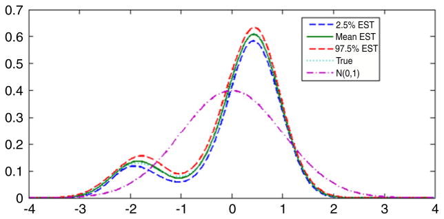
We assessed the performance of the approach through a simulation example designed to mimic the fibroid data described in Section 5.1. In this application, we are interested in inference under the latent factor regression model (13) with the same sample size and x_i values from the real data. For the simulation, we assume that the true parameter values are β = (1, 1, 1, 1)′, Λ = (λ₁, …, λ₇)′ = (1, 1, 1, 1, 1, 1, 1)′ and the latent variable density η_i is the following mixture of four normals:

$$0.15N(-1.92,0.24)+0.05N(-0.95,0.24)+0.15N(0.024,0.24)+0.65N(0.51,0.24)$$

which has mean 0 and variance 1.

The values of X = (x₁, …, x_n) and n are taken directly from the observed data. One of our goals was to assess whether the data contain sufficient information to reliably estimate the latent variable density.

We analyzed the simulation data using a CSBM prior for G, applying the algorithm of Section 4. The DP precision parameter, α, was treated as unknown using a gamma(1, 1) hyperprior, while G₀ was assumed to correspond to N(0, 1). Conditionally conjugate priors were chosen for the remaining parameters as follows:

$$\pi (\mathbf{\mu })={\text{N}}_p(\mathbf{0},10\mathbf{I}),\pi (\mathbf{\lambda })=\prod _{j=1}^p{\text{N}}_{+}({\lambda }_j;0,10),\pi (\mathbf{\tau })=\prod _{j=1}^p\text{gamma}({\tau }_j,1,1),$$

where N₊( m, v) refers to the N (m, v) distribution truncated to (0, ∞), and $\mathbf{\tau }=({\sigma }_1^{-2},\dots ,{\sigma }_p^{-2})$. A blocked Gibbs sampler was implemented in each case, with the chain run for 100,000 iterations after a 20,000 iteration burn-in, we take every 20th sample resulting in a total of 4000 samples. To assess convergence, we ran several independent chains with widely dispersed starting values; for sensitivity to prior specification, we also tried with varied variances: priors with variance/2, priors with variance ×2, priors with variance ×5. With all these trials, we do not see much differences between the results.

Table 1 presents posterior summaries of the model parameters in each case, while Fig. 1 plots the estimated and true latent variable distributions. From these results, we can see that our approach can produce good results. The estimated latent variable density is very close to the true density, suggesting that the data are informative.

Table 1.

Parameter estimation of DPM & CDPM for simulation.

Parameter	True value	DPM		CDPM
		Estimate	95% CI	Estimate	95% CI
β1	1.00	1.66	(1.27, 2.09)	0.88	(0.68, 1.07)
β2	1.00	1.61	(1.26, 2.00)	0.85	(0.68, 1.01)
β3	1.00	1.76	(1.38, 2.24)	0.93	(0.74, 1.14)
β4	1.00	1.73	(1.44, 2.11)	0.92	(0.78, 1.05)
λ1	1.00	0.54	(0.44, 0.63)	1.02	(0.89, 1.15)
λ2	1.00	0.56	(0.46, 0.65)	1.06	(0.92, 1.20)
λ3	1.00	0.56	(0.45, 0.67)	1.06	(0.91, 1.21)
λ4	1.00	0.58	(0.48, 0.69)	1.10	(0.94, 1.29)
λ5	1.00	0.62	(0.48, 0.79)	1.18	(0.97, 1.42)
λ6	1.00	0.61	(0.49, 0.72)	1.14	(0.98, 1.32)
λ7	1.00	0.58	(0.47, 0.68)	1.09	(0.95, 1.24)

Fig. 1.

True and estimated latent variable densities in simulation example.

The centered Dirichlet process mixture (CDPM) model results are much more accurate than the results for the DPM model, as expected due to the non-identifiability problem. In general, the closer the latent variable distribution is to the base G₀, the better the performance of the DPM model. However, the performance of the DPM degrades in the presence of deviation from G₀, while the CDPM results are robust to the shape of the latent variable density.

5.3. Analysis of real data

We implemented the analysis as in the simulation example, and again found the results robust to the prior specification. Posterior summaries of the parameters are provided in Table 3. These results suggest a significant increase in bleeding intensity with increasing fibroid size and for African American women compared with other races. For small fibroids compared with no fibroids, the expected change in the latent bleeding intensity score is 0.05 and the 95% credible interval (CI) includes 0. Note that the latent variable regression coefficients have a clear interpretation due to the incorporation of the variance = 1 constraint. In particular, the coefficients for the indicators represent the number of standard deviations the mean bleeding intensity score shifts between the categories. Hence, a shift of 0.05 is clearly not a clinically significant change. However, the estimated shift of β̂₁ + β̂₂ = 0.05+0.45 = 0.50 between no fibroids and size category 2 is significant. The estimated shift between no fibroids and size category 3 is β̂₁ + β̂₂ + β̂₃ = 1.26. Hence, fibroid size explains a sizable proportion of the variability in the latent bleeding score.

Table 3.

Parameter estimation of DPM & CDPM for real data analysis.

Parameter	DPM		CDPM
	Estimate	95% CI	Estimate	95% CI
β1	0.065	(−0.21, 0.35)	0.05	(−0.18, 0.28)
β2	0.53	(0.29, 0.91)	0.45	(0.25, 0.66)
β3	0.91	(0.60, 1.45)	0.76	(0.51, 1.01)
β4	0.54	(0.34, 0.87)	0.46	(0.28, 0.63)
λ1	0.51	(0.27, 0.71)	0.60	(0.43, 0.83)
λ2	0.018	(0.00, 0.06)	0.02	(0.00, 0.04)
λ3	1.17	(0.73, 1.55)	1.37	(1.04, 1.86)
λ4	0.02	(0.00, 0.07)	0.02	(0.00, 0.02)
λ5	0.12	(0.05, 0.19)	0.14	(0.06, 0.14)
λ6	0.96	(0.61, 1.23)	1.13	(0.88, 1.50)
λ7	0.80	(0.51, 1.01)	0.93	(0.73, 1.23)

Interestingly, African American ethnicity is also a significant predictor of bleeding intensity, even adjusting for fibroid size. Although it is known that African Americans have a higher fibroid prevalence, so that it would not be surprising to see more fibroid related bleeding, the occurrence of higher bleeding rates adjusting for fibroid sizes is interesting. It may be that future development of fibroids between the screening examination and the measurement of bleeding symptoms at the follow-up time may explain this difference.

The estimated latent bleeding intensity residual density is plotted in Fig. 2. Interestingly, the density is quite similar to a normal density, though we have demonstrated power to detect non-normality in the simulation example.

Fig. 2.

Estimated density of the latent bleeding intensity score in the fibroid data application.

It is important to assess which symptoms provide the most information about the latent bleeding intensity score for a woman and hence are most sensitive to fibroid size. With this goal in mind, we plot the predicted mean symptom score in different fibroid size categories for African American women in Fig. 3. The plot for white women and other ethnicities shows a very similar pattern. For symptoms 2, 4 and 5, there are essentially no differences across the fibroid size categories and the factor loading parameters are low, suggesting that the bleeding intensity score has low correlation with these symptoms. Symptoms 2 and 4 relate to spotting, while symptom 5 relates to frequency of menstrual periods. In contrast, for symptom 1, there is a moderate shift across fibroid size categories, while for symptoms 3, 6 and 7, the shift is large, with non-overlapping 95% predictive intervals. These findings are quite plausible biologically, as symptoms 3 and 6 relate to frequency of severe bleeding, while symptom 7 measures bleeding that is sufficient to limit activities.

Fig. 3.

Comparison of bleeding symptoms for black women with large fibroid size (solid line, diamond: estimated mean) vs. no fibroids (dashed line, square: estimated mean).

6. DDT and premature delivery study

6.1. Scientific background and data description

As a second example, we analyzed data from an epidemiology study investigating the relationship between DDT exposure and premature delivery (Longnecker et al., 2001). The study measured concentrations of p, p′-DDT and p, p′-DDE (1, 1-dichloro-2, 2-bis(p-chlorophenyl) ethylene), a persistent metabolite of DDT, in 2613 third trimester maternal serum samples from the US Collaborative Perinatal Project (CPP). Although Longnecker et al. (2001) focused their analysis on serum concentration of p, p′-DDE (x_i1), data were also collected on lipid-adjusted p, p′-DDE (x_i2), serum concentration of p, p′-DDT (x_i3), and lipid-adjusted p, p′-DDT (x_i4). The x_i1, x_i2, x_i3, x_i4 variables are moderately to highly correlated, and it is not clear which should be used in assessing the relationship between DDT exposure and premature delivery.

For this reason, it is natural to consider a latent variable model of the form:

$$\begin{array}{l}\text{logit}\{\text{Pr}(y_i=1\mid {\eta }_i,{\mathbf{z}}_i)\}={\mathbf{z}}_i^{\prime }{\mathbf{\tau }}_y+{\lambda }_y{\eta }_i\\ x_{ij}={\tau }_{x,j}+{\lambda }_{x,j}{\eta }_i+{\epsilon }_{ij},{\epsilon }_{ij}~N(0,{\sigma }_j^2),j=1,2,3,4\\ {\eta }_i~G,\end{array}$$ (15)

where y_i = 1 if woman i experiences a preterm birth and y_i = 0 otherwise, z_i is a vector of predictors with z_i = (1, age_i, black_i)′, age_i is standardized age for woman i, black_i is an indicator of African American ethnicity, η_i is a latent variable summarizing the level of DDT exposure, λ_y is a coefficient characterizing the effect of η_i on the log-odds of preterm birth, and G is the distribution of η_i. Mean and variance constraints on G are necessary to fix the scale of the latent variable, which is needed for identifiability and interpretability of the λ_y coefficient. If G has mean zero and variance one, then λ_y is interpretable as the increase in log-odds of preterm birth attributable to a one standard deviation increase in exposure, and z′ τ_y is the baseline log-odds of preterm birth among individuals with an average level of exposure having predictors z.

To provide further motivation, DDT is a pesticide, which is currently banned in the United States and numerous countries. However, DDT is still in routine use in the developing world as an anti-malarial agent due to its effectiveness against mosquitoes. Decisions to continue the use of DDT must weigh this public health benefit against the increasing evidence of adverse human health effects.

Our interest focuses on investigating the impact on preterm delivery, which is a major public health concern worldwide, as babies born premature are at substantially increased risk of infant mortality as well as short and long term morbidity. In addition, extended hospital stays and care associated with prematurity is extremely expensive. In assessing public health impact and conveying this impact to clinicians and policy makers, it is important to have a simple and interpretable summary of association between DDT exposure and risk of prematurity.

It is not possible to accurately measure the level of external exposure to DDT for different women in a large, prospective epidemiologic study, such as the US Collaborative Perinatal Project (CPP). Instead, Longnecker et al. (2001) relied on assaying maternal serum samples collected in the third trimester of pregnancy. Blood levels of p, p′-DDT and the persistent metabolite, p, p′-DDE, provide surrogates of the external exposure to DDT, with the health impact of the external exposure being the primary interest from a public health perspective. Because p, p′-DDT and p, p′-DDE are lipid-soluble, there has been some controversy in the literature over whether one should basis the analysis on serum levels in μg/L or on lipid-adjusted values. As there are valid arguments on both sides, our preference is to include both types of measurements through the latent variable model (15).

An additional argument in favor of the latent variable model (15) is interpretability. As an overall measure of the association between p, p′-DDE and preterm birth, one can present an estimated logistic regression coefficient, say θ̂. The coefficient θ is interpretable as the increase in the log-odds of preterm birth attributable to a one μg/L increase in serum level of p, p′-DDE. Unfortunately, the value of θ̂ provides no insight into public health impact in the absence of careful thinking about the population distribution of p, p′-DDE. In contrast, the coefficient λ_y in model (15) is interpretable as the increase in log-odds of exposure due to a one standard deviation increase in the summary measure of exposure to DDT.

6.2. Simulation experiment

For comparison, as in Section 5.2, we repeated the analysis under the assumption that the latent variable had a N(0, 1) density instead of an unknown density. Fig. 5 presents the estimated and true latent variable densities in comparison with the standard normal. It is clear that the data contain substantial information about the latent variable density in that we obtained a very accurate estimate of the density in this simulation, which was chosen to have the same sample size and data structure as the DDT and preterm birth application presented in Section 6. Table 4 provides posterior summaries of the parameters in the CDPM and normal latent variable analysis. Most of the parameter estimates seemed robust to misspecification of the latent variable density in that the normal analysis produced posterior means close to the true values for the factor loadings, residual variances, and intercepts in the predictor model. However, as shown in Fig. 6 there was evidence of bias in estimation of the exposure effect coefficient, λ_y, which would be the primary interest in most applications. For the CDPM analysis, the posterior density of λ_y was centered on the true value of 0.2, while in the normal analysis the true value was in the right tail of the posterior. Although the results are not presented here, the uncentered DPM produced poor results in this and other simulation cases we considered.

Fig. 5.

True and estimated latent variable densities for the simulation example. The dotted line is the posterior mean estimate, the solid line is the true density, and the dashed lines are 95% pointwise credible intervals.

Table 4.

Summaries of the posterior distributions under the normal latent factor model and the centered Dirichlet process mixture latent factor model for data simulated to mimic the DDT and premature delivery data.

Parameter	True value	Normal		CDPM
		Estimate	95% CI	Estimate	95% CI
τy,1	−2.2	−2.09	(−2.43, −1.85)	−2.19	(−2.71, −2.03)
τy,2	0.10	0.11	(0.08, 0.11)	0.10	(0.09, 0.12)
τy,3	1.00	1.12	(0.98, 1.24)	1.03	(0.95, 1.20)
λy,1	0.20	0.15	(0.09, 0.21)	0.20	(0.13, 0.26)
λx,1	1.00	0.99	(0.94, 1.04)	1.01	(0.97, 1.06)
λx,2	2.00	2.01	(1.94, 2.08)	1.99	(1.92, 2.06)
λx,3	3.00	3.01	(2.92, 3.11)	3.00	(2.93, 3.10)
λx,4	4.00	4.01	(3.88, 4.13)	3.99	(3.89, 4.11)
σx,1	1.00	1.01	(0.98, 1.04)	0.98	(0.95, 1.01)
σx,2	1.00	0.98	(0.96, 0.99)	1.01	(0.99, 1.04)
σx,3	1.00	0.96	(0.92, 1.02)	0.97	(0.93, 1.01)
σx,4	1.00	0.99	(0.94, 1.07)	1.02	(0.98, 1.09)
τx,1	0.00	0.00	(−0.06, 0.06)	0.00	(−0.06, 0.05)
τx,2	0.00	−0.01	(−0.08, 0.08)	−0.04	(−0.13, 0.04)
τx,3	0.00	−0.04	(−0.17, 0.08)	−0.05	(−0.16, 0.08)
τx,4	0.00	−0.01	(−0.17, 0.14)	−0.06	(−0.16, 0.05)

Fig. 6.

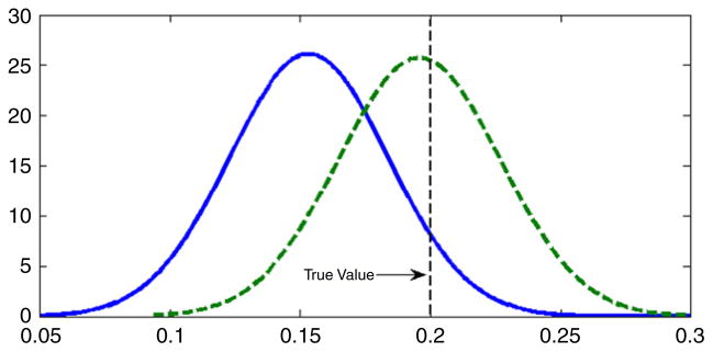
Estimated posterior densities for λ_y in the simulation example. The dotted line is the density in the normal analysis, and the solid line is the density in the CDPM analysis. The vertical line shows the true value.

6.3. Analysis and results

The Longnecker et al. (2001) study had serum measurements for 2613 women selected from the CPP. Our analysis focused on 2380 women, obtained after removing 233 women who had missing covariate values. Data for a single pregnancy was available for each woman, with 361/2380 = 15% of the pregnancies resulting in a preterm birth. The average age for women in the sample was 24, with an interquartile range of 20–28.

Fig. 4 shows histograms for x_i1 − x_i4, while Table 6 shows the correlations in the different DDT surrogates. It is clear from Fig. 4 that the surrogates are not normally distributed and there is a tendency towards a large right skew in the distributions. In addition, the surrogates are moderately to highly correlated, providing support for the incorporation of a single summary latent variable η_i in model (15). The women in the right tail of the distribution for one surrogate tended to be in the right tail for the other surrogates.

Fig. 4.

Histograms of the DDT data.

Table 6.

DDT surrogates correlation table.

	xi1	xi2	xi3	xi4
xi1	1.00	0.91	0.69	0.61
xi2	0.91	1.00	0.61	0.70
xi3	0.69	0.61	1.00	0.91
xi4	0.61	0.70	0.91	1.00

To minimize the influence of subjective hyperparameter selection, which was necessary to avoid the possibility of an improper posterior, we standardized the surrogates prior to analysis. A repeat analysis without standardization did not change the results. We implemented the analysis for the CDPM and normal latent variable models using the same prior and computational implementation as that described in Section 5. Table 5 presents posterior summaries for each of the parameters. In both the normal and CDPM analysis, there was no association between preterm birth and age, likely due to the fact that women in the sample were primarily young. In addition, the analyses estimated a 0.26–0.27 increase in the log-odds of preterm birth among African Americans. It is well known in the literature that African American’s tend to have consistently higher rates of preterm birth.

Table 5.

Posterior summaries under the normal latent factor model and the centered DPM latent factor model for the DDT and preterm birth data.

Parameter	Normal		CDPM
	Estimate	95% CI	Estimate	95% CI
τy,1	−1.11	(−1.39, −0.84)	−1.14	(−1.42, −0.87)
τy,2	0.00	(−0.01, 0.00)	0.00	(−0.01, 0.01)
τy,3	0.27	(0.13, 0.41)	0.26	(0.12, 0.40)
λy	0.14	(0.07, 0.20)	0.11	(0.05, 0.18)
λx,1	0.95	(0.92, 0.98)	0.71	(0.65, 0.79)
λx,2	0.95	(0.92, 0.99)	0.74	(0.67, 0.81)
λx,3	0.72	(0.69, 0.76)	0.96	(0.89, 1.05)
λx,4	0.74	(0.70, 0.78)	0.98	(0.90, 1.07)
σx,1	0.33	(0.30, 0.34)	0.70	(0.68, 0.73)
σx,2	0.30	(0.28, 0.32)	0.68	(0.66, 0.70)
σx,3	0.70	(0.68, 0.72)	0.34	(0.32, 0.36)
σx,4	0.69	(0.66, 0.71)	0.28	(0.26, 0.31)
τx,1	0.00	(−0.04, 0.04)	0.00	(−0.04, 0.04)
τx,2	0.00	(−0.04, 0.04)	0.00	(−0.04, 0.04)
τx,3	0.00	(−0.04, 0.05)	0.00	(−0.03, 0.05)
τx,4	0.00	(−0.04, 0.05)	0.00	(−0.03, 0.05)

The results of the parametric and CDPM analysis were much less consistent for the parameters characterizing the relationship between the latent variable, η_i, and the measured variables, y_i and x_i = (x_i1, x_i2, x_i3, x_i4)′. As shown in Fig. 8, there is a non-negligible shift in the posterior distribution for λ_y, with the normal analysis producing an estimate of λ̂_y = 0.14 (95% CI = [0.07, 0.20]) and the CDPM analysis resulting in λ̂_y = 0.11 (95% CI = [0.05, 0.18]). In both cases, there is a clear increase in the risk of preterm birth as level of exposure increases, and 95% credible intervals have similar widths, suggesting that the nonparametric approach does not in general result in a reduction in efficiency. In fact, we have observed in other cases that the credible intervals are commonly narrower for the nonparametric analysis in cases in which the parametric model provides a poor approximation.

Fig. 8.

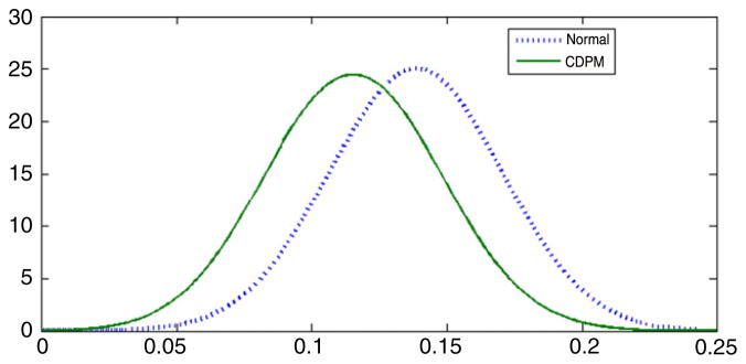
Estimated posterior densities for λ_y in the DDT and preterm birth application. The solid line is the estimate in the CDPM analysis, while the dotted line is the estimate for the normal latent variable model.

Fig. 7 shows the estimated latent variable density along with pointwise 95% credible intervals. Clearly, there are substantial departures from normality, with the latent variable density having a large right skew consistent with the surrogate distributions shown in Fig. 4 and with exploratory analyses of the data. It appears that many individuals have a low level of exposure to DDT, but there are a few individuals with very high levels of exposure. This is certainly a common scenario in epidemiology. We note that log transforming the surrogate data results in a latent variable density that is closer to normal, but with clear departures. Post hoc choices of transformations can result in an underestimation of uncertainty and biased inferences, and we find it unappealing to obscure the large differences in exposure level through a transformation that reduces the right tail. In addition to obtaining a very different estimate of the latent variable density under our semiparametric Bayes analysis, we also note that the variance component estimates are substantially different than those obtained in the normal latent variable analysis. This is apparent in examining Table 3.

Fig. 7.

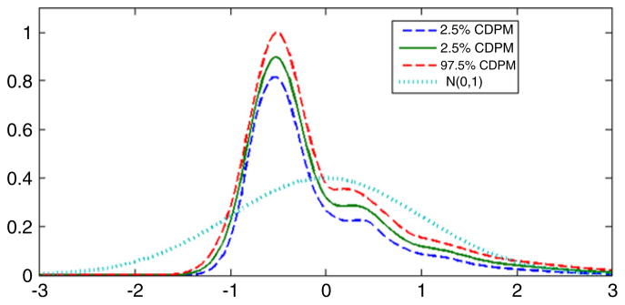
Estimated density of the latent DDT exposure variable in the DDT and premature birth application. The solid line is the posterior mean, the dashed lines are 95% pointwise credible intervals, and the dotted line is the standard normal density.

We repeated the convergence assessments and sensitivity analyses reported in Section 5, and obtained very similar results. In particular, rates of convergence and mixing were quite good based on examination of trace plots and standard diagnostics, and inferences were not sensitive to local changes in the hyperparameter choice.

7. Discussion

In this article, we propose a centered stick-breaking process that constrains the mean and variance for latent variable distributions in a hierarchical model. We accomplish this method with the use of parameter expansion, that is, by viewing the uncentered stick-breaking process as a parameter-expanded version of the centered stick-breaking process. This is a simple but useful idea that has a clear impact on the results, reducing bias and improving interpretability over uncentered methods. An appealing feature is that approximate posterior computation can proceed as in the uncentered case with a very simple post-processing algorithm applied to the MCMC draws. This bypasses the need to implement computation directly for the constrained model, which is very challenging.

Appendix

Here, we present the conditional posterior distribution used in implementing the Gibbs sampler for the following models:

$$\begin{array}{l}{y}_{ij}={\tau }_j+{\lambda }_j{\eta }_i+{\epsilon }_{ij},{\epsilon }_{ij}~N(0,{\sigma }_j^2)\\ {\eta }_i={\mathbf{x}}_i\mathbf{\beta }+{\mu }_i+{\delta }_i,{\delta }_i~N(0,1),{\mu }_i~G.\end{array}$$

• With prior ${\tau }_j~N({\mu }_{\tau },{\sigma }_{\tau }^2)$, the posterior is $N({\mu }_{\tau }^{\ast },{\sigma }_{\tau }^{\ast 2})$.

  $$\begin{array}{l}{\sigma }_{\tau }^{\ast -2}={\sigma }_{\tau }^{-2}+{\eta }_j{\sigma }_j^{-2}\\ {\mu }_{\tau }^{\ast }={\sigma }_{\tau }^{\ast 2}\left\{{\mu }_{\tau }{\sigma }_{\tau }^{-2}+\sum _{i=1}^n{\sigma }_{\tau }^{-2}(y_{ij}-{\lambda }_j{\eta }_i)\right\}.\end{array}$$
• For prior ${\lambda }_j~N_{+}({\mu }_{\lambda },{\sigma }_{\lambda }^2)$, the posterior is truncated positive normal with parameters

  $$\begin{array}{l}{\sigma }_{\lambda }^{\ast -2}={\sigma }_{\lambda }^{-2}+\sum _{i=1}^{n_j}{\eta }_i^2/{\sigma }_j^2\\ {\mu }_{\lambda }^{\ast }={\sigma }_{\lambda }^{\ast 2}\left\{{\mu }_{\lambda }{\sigma }_{\lambda }^{-2}+\sum _{i=1}^{n_j}{\eta }_i{\sigma }_j^{-2}(y_{ij}-{\tau }_j)\right\}.\end{array}$$
• For prior ${\sigma }_j^2~\text{IG}(d_1,d_2)$, the posterior is also inverse-gamma distribution with parameters

  $$\begin{array}{l}{d}_1^{\ast }=d_1+n_j/2\\ d_2^{\ast }=d_2+\sum _{i=1}^{n_j}{(y_{ij}-{\tau }_j-{\lambda }_j{\eta }_i)}^2/2.\end{array}$$
• Sample η_i from the posterior normal distribution with parameters

  $$\begin{array}{l}{\sigma }_{{\eta }_i}^{\ast -2}=1.0+\sum _{j=1}^p{\lambda }_j^2/{\sigma }_j^2\\ {\mu }_{{\eta }_i}^{\ast }={\sigma }_{{\eta }_i}^{\ast 2}\left\{{\mathbf{x}}_i^{\prime }\mathbf{\beta }+{\mu }_i+\sum _{j=1}^p{\lambda }_j{\sigma }_j^{-2}(y_{ij}-{\tau }_j)\right\}.\end{array}$$
• With prior of N(β₀, Σ_β0), sample β from the posterior normal distribution with parameters

  $$\begin{array}{l}{\mathbf{\sum }}_{\mathbf{\beta }}^{\ast -1}={\mathbf{xx}}^{\prime }+{\mathbf{\sum }}_{{\mathbf{\beta }}_0}^{-1}\\ {\mathbf{\mu }}_{\mathbf{\beta }}^{\ast }={\mathbf{\sum }}_{\mathbf{\beta }}^{\ast }\left\{{\mathbf{\sum }}_{{\mathbf{\beta }}_0}^{-1}{\mathbf{\beta }}_0+\sum _{i=1}^n{\mathbf{x}}_i({\eta }_i-{\mu }_i)\right\}.\end{array}$$
• The unique values of ${\mathbf{\mu }}^{\ast }=({\mu }_1^{\ast },\dots ,{\mu }_N^{\ast })$, which corresponds to μ = (μ₁, …, μ_n), n ≥ N. With prior N(g1, g2), we sample the posterior ${\mu }_i^{\ast }$ from normal distribution with parameters

  $$\begin{array}{l}{g}_2^{\ast }=g_2^{-1}+\sum _{i:{\mu }_i={\mu }_j^{\ast }}{\mu }_j^{\ast 2}\\ g_1^{\ast }=g_2^{\ast }\left\{g_1/g_2+\sum _{i:{\mu }_i={\mu }_j^{\ast }}({\eta }_i-{\mathbf{x}}_i\mathbf{\beta })\right\}.\end{array}$$
• Allocate individuals to latent classes for ${\mu }_i^{\ast }$ by sampling $K_i^{\ast }$ from

  $$\begin{array}{l}{K}_i^{\ast }~\sum _{k=1}^N{p}_{K,i}{\delta }_k(·)\\ p_{k,i}\propto p_{k}N({\eta }_i\mid {\mathbf{x}}_i\mathbf{\beta }+{\mu }_i,1.0).\end{array}$$

• Sample $V_j^{\ast }$ from posterior Beta distribution $V_j^{\ast }~\text{Beta}(1.0+q_j,c+{\sum }_{l=j+1}^N{q}_l)$, j = 1, …, N − 1, where $q_j={\sum }_{i=1}^{n}I({\mu }_i={\mu }_j^{\ast })$. Set $p_1=V_1^{\ast },\dots ,p_j=(1-V_1^{\ast })(1-V_2^{\ast })\cdots (1-V_{j-1}^{\ast })V_j^{\ast }$ for j = 2, …, N − 1.

• With prior gamma(g, h), sample c from posterior gamma with parameters

  $$\begin{array}{l}{g}^{\ast }=g+N\\ h^{\ast }=h-\sum _{i=1}^{N}log(1-V_i^{\ast }).\end{array}$$

References

- Baird DD, Dunson DB, Hill MC, Cousins D, Schectman JM. High cumulative incidence of uterine leiomyoma in black and white women: ultrasound evidence. American Journal of Obstetrics and Gynecology. 2003;188:100–107. doi: 10.1067/mob.2003.99. [DOI] [PubMed] [Google Scholar]
- Bhattacharya A, Dunson DB. Discussion Paper. Vol. 23. Department of Statistical Science, Duke University; Durham, NC: 2009. Sparse Bayesian infinite factor models. [Google Scholar]
- Brunner L, Lo A. Bayes methods for a symmetric unimodal density and its mode. The Annals of Statistics. 1989;17:1550–1566. [Google Scholar]
- Burr D, Doss H. A Bayesian semiparametric model for random-effects meta-analysis. Journal of the American Statistical Association. 2005;100:242–251. [Google Scholar]
- Bush CA, MacEachern SN. A semiparametric Bayesian model for randomized block designs. Biometrika. 1996;83:275–285. [Google Scholar]
- Doss H. Bayesian nonparametric estimation of the median: part 1: computation of the estimates. The Annals of Statistics. 1985;13:1432–1444. [Google Scholar]
- Dunson DB. Bayesian latent variable models for clustered mixed outcomes. Journal of the Royal Statistical Society B. 2000;62:355–366. [Google Scholar]
- Dunson DB, Watson M, Taylor JA. Bayesian latent variable models for median regression on multiple outcomes. Biometrics. 2003;59:296–304. doi: 10.1111/1541-0420.00036. [DOI] [PubMed] [Google Scholar]
- Escobar M. Estimating normal means with a Dirichlet process prior. Journal of the American Statistical Association. 1994;89:268–277. [Google Scholar]
- Escobar M, West M. Bayesian density estimation and inference using mixtures. Journal of the American Statistical Association. 1995;90:577–588. [Google Scholar]
- Ferguson TS. A Bayesian analysis of some nonparametric problems. The Annals of Statistics. 1973;1:209–230. [Google Scholar]
- Ferguson TS. Prior distributions on spaces of probability measures. The Annals of Statistics. 1974;2:615–629. [Google Scholar]
- Gelman A. Parameterization and Bayesian modeling. Journal of the American Statistical Association. 2004;99:537–545. [Google Scholar]
- Gelman A. Prior distributions for variance parameters in hierarchical models. Bayesian Analysis. 2006;1:515–534. [Google Scholar]
- Hanson T, Johnson WO. Modeling regression error with a mixture of polya trees. Journal of the American Statistical Association. 2002;97:1020–1033. [Google Scholar]
- Hoff PD. Doctoral Dissertation. Department of Statistics, University of Wisconsin; 2000. Constrained nonparametric estimation via mixtures. [Google Scholar]
- Hoff PD. Nonparametric estimation of convex models via mixtures. The Annals of Statistics. 2003;31:174–200. [Google Scholar]
- Ishwaran H, James LF. Gibbs sampling methods for stick-breaking priors. Journal of the American Statistical Association. 2001;96:161–173. [Google Scholar]
- Ishwaran H, Takahara G. Independent and identically distributed Monte Carlo algorithms for semiparametric linear mixed models. Journal of the American Statistical Association. 2002;97:1154–1166. [Google Scholar]
- James LF. Functionals of Dirichlet processes, the Cifarelli–Regazzini identity and beta–gamma processes. The Annals of Statistics. 2005;33:647–660. [Google Scholar]
- Kleinman KP, Ibrahim JG. A semiparametric Bayesian approach to the random effects model. Biometrics. 1998;54:921–938. [PubMed] [Google Scholar]
- Kottas A, Gelfand AE. Bayesian semiparametric median regression modeling. Journal of the American Statistical Association. 2001;96:1458–1468. [Google Scholar]
- Lavine M. On an approximate likelihood for quantiles. Biometrika. 1995;82:220–222. [Google Scholar]
- Lavine M, Mockus A. A nonparametric Bayes method for isotonic regression. Journal of Statistical Planning and Inference. 1995;46:235–248. [Google Scholar]
- Li Y, Muller P, Lin X. Technical Report. 2007. Bias-Corrected Inference in Semiparametric Bayesian Mixed Models. [Google Scholar]
- Liu JS, Wu YN. Parameter expansion for data augmentation. Journal of the American Statistical Association. 1999;94:1264–1274. [Google Scholar]
- Lopes HF, West M. Bayesian model assessment in factor analysis. Statistica Sinica. 2004;14:41–67. [Google Scholar]
- Longnecker MP, Klebanoff MA, Zhou HB, Brock JW. Association between maternal serum concentration of the DDT metabolite DDE and preterm and small-for-gestational-age babies at birth. Lancet. 2001;358:110–114. doi: 10.1016/S0140-6736(01)05329-6. [DOI] [PubMed] [Google Scholar]
- Moustaki I, Knott Generalized latent trait models. Psychometrika. 2000;65:391–441. [Google Scholar]
- Mukhopadhyay S, Gelfand AE. Dirichlet process mixed generalized linear models. Journal of the American Statistical Association. 1997;92:633–639. [Google Scholar]
- Müller P, Rosner G. A Bayesian population model with hierarchical mixture priors applied to blood count data. Journal of the American Statistical Association. 1997;92:1279–1292. [Google Scholar]
- Pison G, Rousseeuw PJ, Flizmoser P, Croux C. Robust factor analysis. Journal of Multivariate Analysis. 2003;84:145–172. [Google Scholar]
- Pison G, Van Aelst S. Diagnostic plots for robust multivariate methods. Journal of Computational and Graphical Statistics. 2004;13:310–329. [Google Scholar]
- Regazzini E, Guglielmi A, Di Nunno G. Theory and numerical analysis for exact distributions of functionals of a Dirichlet process. The Annals of Statistics. 2002;30:1376–1411. [Google Scholar]
- Sethuraman J. A constructive definition of the Dirichlet process. Statistica Sinica. 1994;4:639–650. [Google Scholar]
- Wegienka G, Baird D, Hertz-Picciotto I, Harlow S, Steege J, Hill M, Schectman M, Hartmann K. Self-reported heavy bleeding associated with uterine leiomyomata. American Journal of Obstetrics and Gynecology. 2003;3:431–437. doi: 10.1016/s0029-7844(02)03121-6. [DOI] [PubMed] [Google Scholar]
- West M. Bayesian factor regression models in the large p, small n paradigm. Bayesian Statistics. 2003;7:723–732. [Google Scholar]