

Abstract
Understanding the mechanisms underlying the observed dynamics of complex biological systems requires the statistical assessment and comparison of multiple alternative models. Although this has traditionally been done using maximum likelihood-based methods such as Akaike's Information Criterion (AIC), Bayesian methods have gained in popularity because they provide more informative output in the form of posterior probability distributions. However, comparison between multiple models in a Bayesian framework is made difficult by the computational cost of numerical integration over large parameter spaces. A new, efficient method for the computation of posterior probabilities has recently been proposed and applied to complex problems from the physical sciences. Here we demonstrate how nested sampling can be used for inference and model comparison in biological sciences. We present a reanalysis of data from experimental infection of mice with Salmonella enterica showing the distribution of bacteria in liver cells. In addition to confirming the main finding of the original analysis, which relied on AIC, our approach provides: (a) integration across the parameter space, (b) estimation of the posterior parameter distributions (with visualisations of parameter correlations), and (c) estimation of the posterior predictive distributions for goodness-of-fit assessments of the models. The goodness-of-fit results suggest that alternative mechanistic models and a relaxation of the quasi-stationary assumption should be considered.
Introduction
Model comparison
Model-based inference is widely used in life sciences in order to assess the plausibility of hypothesised biological mechanisms based on data from observations or experiments. One of the most common approaches to compare competing models representing alternative hypotheses relies on Akaike's Information Criterion (AIC) [1]. For a given data set  , the plausibility of the candidate models
  is assessed by calculating their respective AIC values,
  :
:
| (1) |
In (1),  is the maximum likelihood estimate of the set parameters associated with model
  , and
, and  is the corresponding number of degrees of freedom. If
  then
then  is more plausible than
  , with respect to
  , in the sense that the Kullback-Liebler divergence of
  from the true model is smaller [2].
An important drawback to the classic approach to model choice is that it is based on a single point estimate  of
of  , the uncertainty in
  being ignored. In contrast, the Bayesian approach considers a probability distribution for
  , with
  expressing the uncertainty in
  given
given  (for a model
  ).
).
Suppose that we wish to select a model from a set of candidate models  given our observation of data
  . We can express this goal probabilistically by stating that the aim is to determine the most probable model:
  .
.
From Bayes' theorem, we have
| (2) |
therefore, if  is known, or considered to be equal for all
  then the focus is on the model evidence
  .
.
If  is the set of parameters associated with model
  , the Bayesian approach to
  is to integrate over all possible values of
  :
:
| (3) |
In addition to allowing for parameter uncertainty, (3) intrinsically penalizes against models that are better able to fit to observed data because of their complexity [3], thereby removing the need for an explicit complexity penalization term.
The integral of (3) can be estimated analytically or numerically. In analytical approaches, the integral is approximated by the adoption of simplifying assumptions; for example, as used for derivation of the Bayes Information Criterion [4]. Numerical approaches are based on some form of Monte Carlo sampling such as Gibbs Sampling [5].
One approach to estimating the integral
 |
numerically is to sample  randomly from its prior,
| (4) |
however, the prior  is often concentrated in places where the likelihood
  is relatively low. This problem becomes more severe in high-dimensional parameter
  spaces, or in problems where the likelihood function
  is concentrated in a very small region.
To overcome the problem, Skilling [6], [7] proposed a means of estimating  that, by design, samples
  sparsely from the
  space where the likelihood
  is low, and densely where
  is high, by means of ‘nested sampling’, which is the focus of this paper. A recent addition to the Bayesian arsenal, nested sampling has been used in cosmology to compare alternative models of the universe against observed data [8]. Outside of physics, it has, so far, received little attention [9], [10].
Within-host dynamics of a bacterial infection
Quantitative research on infectious disease dynamics has undergone rapid development over the last two decades, motivated by concerns about emerging infections that can spread globally and about the evolution of pathogens resistant to existing control measures such as antimicrobials and vaccines. Bayesian computation has become the method of choice to fit stochastic dynamic models to epidemiological [11] or experimental datasets [12]. This is in large part due to the appeal of being able to produce measures of uncertainty and correlation for the model parameters based on their posterior probability distributions. Similarly, models for within-host dynamics of infection have more recently started to benefit from Bayesian inference approaches [13].
Salmonella enterica causes systemic diseases (typhoid and paratyphoid fever) [14], food-borne gastroenteritis and non-typhoidal septicaemia (NTS) [15] in humans and in many other animal species world-wide, which also cause a very serious problem for the food industry. The global burden of typhoid fever is estimated at ca. 22 million cases with a mortality estimated at ca. 200,000 deaths per year [14], [16]. Paratyphoid has an estimated 5.4 million illnesses worldwide [16]. The high incidence of these diseases, that affect both travellers to and residents in endemic areas, and threaten infants, children and immunodeficient patients, dictates the urgent need for more efficacious preventive and therapeutic measures.
In the mouse model of systemic infection, Salmonella reside and proliferate mainly within phagocytic cells of the spleen liver, bone marrow and lymph nodes [17]–[19]. Observation of Salmonella by fluorescence microscopy in the tissues of mice has revealed that a key feature of systemic infections with wild type bacteria is the presence, on average, of low bacterial numbers within individual phagocytes irrespective of net bacterial growth rate and time since infection [20]–[23].
In an effort to understand the dynamics that underpin the intracellular numerical distributions of Salmonella within the host cells, and to capture the essential traits of the cell-to-cell spread of the bacteria, we have used mathematical model frameworks for the intensity of intracellular infection that links the quasi-stationary distribution of bacteria to bacterial and cellular demography. An example of this the work done by Brown et al. [24], who compared the observed distribution  , where
  is the number of cells with
  bacteria, across 16 candidate infection models. The models under consideration were as follows: (a) one homogeneous model, in which, for every cell, burst occurred only when the number of bacteria
  in a cell reached a single burst threshold
  ; (b) five heterogeneous models having a probability distribution of burst thresholds; and (c) eight stochastic models for which there is a probability that a given cell will undergo burst. Two datasets were analysed, one for a virulent strain of bacteria and the other for an attenuated strain. Brown et al. [24] computed the maximum likelihood estimates of the parameters of each model, and selected the ‘best’ model based on the corresponding AIC values.
In order to overcome the issues raised by AIC discussed above, we decided to re-analyse the datasets and re-assess the models within a Bayesian framework.
Methods
What follows is an elaboration of the description of nested sampling given by Skilling [6], [7].
Nested sampling
The expected value of a function  of a random variable
  is given by
where  is the pdf of
  . On comparing this expression with the target integral
  , it is clear that
| (5) |
that is to say, the expected value of the likelihood under the prior. The cumulative distribution function  with respect to a random variable
  is defined by
and is related to the expectation  by
by
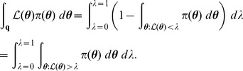
[25]; consequently, from (5), we obtain the important relationship
| (6) |
where  is likelihood, and
  in the right-hand integral is equal to
  . The reason why (6) is important is that the multivariate integral on the left-hand side has been equated to a univariate integral.
Since  has a distribution defined by prior
  , and
, and  , it follows that
  has a probability distribution and thus a cumulative distribution function,
| (7) |
which is present in the integrand of the right-hand integral of (6).
We can replace  in (6) with a more accessible integral by the following steps. First, since the pdf of
  is connected to the pdf of
  via
via  , we can write
| (8) |
thus, from (6), (7) and (8), we can write
 |
(9) |
It will be convenient to rewrite the inner integral of (9) as  to give
| (10) |
where  is the probability of selecting
  from the prior
  such that
  :
:
| (11) |
Introducing  , hence
  , we can rewrite the previous integral as
| (12) |
where  is that likelihood
  such that
  (cf. Equation (11)); for example, if
  then 90% of
  drawn from the prior
  will have likelihoods greater than 0.0042.
The algorithm
The main steps of the nested sampling technique are as follows. First,  points
  (i.e., parameter vectors) are sampled from the prior
  , and their corresponding likelihoods
  determined. The point
  having the smallest likelihood is determined and its likelihood
  is recorded. Furthermore, the probability
  that
that  is also recorded.Point
  is replaced by a new
  drawn from the prior
  but restricted to those
  for which
  . In other words, a restricted prior is used:
  . If
. If  is the set of all possible
  then the set
 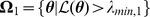 is a subset of
  .
.
The above sequence of determining  and the corresponding
  is performed on the new set of points, giving rise to
  and
and  . Point
  is replaced by a
  drawn from the new restricted prior
  . In other words,
  is sampled from
 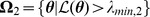 , for which
  .
.
This cycle is repeated until some stopping criterion has been reached. If this termination occurs at the  -th iteration then the resulting values of
  and
and  will be
and the resulting sequence of  subsets is
hence the term nested sampling.
Model evidence 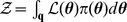 can be estimated from the recorded
  and
and  values by means of the approximation
| (13) |
where  is the number of iterations used, and
  is a vertical rectangular segment under the curve of Figure 1.
Figure 1. The shaded area below the curve for  is equal to
  .
.

See Equation (12).
Algorithm 1 (Table 1) describes the above process in pseudocode.
Table 1. Algorithm 1: The nested sampling algorithm.
Input: (a) likelihood function  ; (b) prior ; (b) prior  ; (c) number ; (c) number  of active parameter vectors in use during nested sampling. of active parameter vectors in use during nested sampling. |
Out put: an estimate  of of  . . |
1: Let  be a set of be a set of  parameter vectors parameter vectors 
|
2: 
|
3: 
|
| 4:while terminating condition not satisfied do |
5: 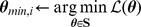
|
6: 
|
7: 
|
8: if
 then
then
|
9:  ▹Estimated segment of ▹Estimated segment of 
|
10: 
|
11:  ▹Restricted prior ▹Restricted prior |
12: 
|
13: 
|
return

|
Practical adjustments to the algorithm
We will now consider how some of the aspects of Algorithm 1 can be implemented.
Segment  used in (13) could be evaluated by the trapezoidal approach
but Sivia and Skilling [26] have found
to be adequate (line 9 in Algorithm 1).
Line 7 in Algorithm 1 used the assignment  , but an alternative approach is to replace this assignment with
  . An approximation of
  is derived as follows. Let
  denote the ratio
  , with
  . At the
  th iteration we have
and so
therefore,
| (14) |
Now,
therefore, from (14),
Since the logarithm function is strictly increasing and concave, we have, from Jensen's inequality, that
and thus
however, Sivia and Skilling [26, p. 186] drop the inequality and use the approximation
As regards the termination of Algorithm 1, there is no rigorous criterion as to when the algorithm should be stopped, but Skilling [7] and Feroz and Hobson [28] have found
to be an effective stopping condition, where  is the fraction of
  that will not significantly contribute to the estimate of
  (according to a user-defined value).
Chopin and Robert [29] have shown that the asymptotic variance of the nested sampling approximation typically grows linearly with parameter dimensions.
Finally, there is the structure of the restricted priors. Each new point  for a set
  of active points is sampled from prior
  conditioned on the restriction that
  . Rather than searching across the entire
  -space for such a point, it is more computationally efficient to restrict the search to a region
  that contains
  . We have used rectangular cuboids for
  .
.
Incorporating the above points into Algorithm 1 leads to Algorithm 2 (Table 2). Before applying the algorithm to our experimental datasets, we tested it on a simple two-parameter likelihood function  . The analyses and results are presented in Methods S1.
Table 2. Algorithm 2: An implementation of Algorithm 1 in which practical adjustments are included.
Input (a) likelihood function  ; (b) prior ; (b) prior  ; (c) number ; (c) number  of active parameter vectors in use during nested sampling; (d) procedure for determining a region of active parameter vectors in use during nested sampling; (d) procedure for determining a region  of parameter space that encloses a set of parameter vectors of parameter space that encloses a set of parameter vectors  ; (e) fraction ; (e) fraction  of of  to be estimated. to be estimated. |
Output: an estimate  of of  . . |
1: Let  be a set of be a set of  parameter vectors parameter vectors 
|
2: 
|
3: 
|
| 4:Repeat |
5: 
|
6: 
|
7: 
|
8: if
 then
then
|
9:  ▹Estimated segment of ▹Estimated segment of 
|
10: 
|
11:  ▹Restricted prior ▹Restricted prior |
12: 
|
13: 
|
14: until:
 ▹The stopping condition ▹The stopping condition |
return

|
The Salmonella models
Evidence  was estimated by nested sampling with respect to two groups of models associated with within-host S. enterica infection, were each model
  provides an expression for the probability
  that a host cell contains
  bacteria.
In the first group of models, infected cells are assumed to burst when the number of bacteria they contain reach a fixed threshold  . The probability distributions considered for
  are shown in Table 3.
Table 3. Probability distributions  for the burst thresholds
  .
.
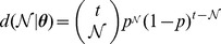
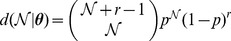
| Model | Distribution | Parameters, θ |
| 1 |

|
|
| 2 |

|
 , ,  , , 
|
| 3 |

|

|
| 4 |
|
 , , 
|
| 5 |
|
 , , 
|
| 6 |
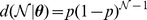
|

|
(1) Unimodal Kronecker, (2) bimodal Kronecker, (3) Poisson, (4) binomial, (5) negative binomial, and (6) geometric.
For the second group of models, the assumption is that, instead of pre-programmed burst thresholds  , there is burst rate
  that is a function of the number of bacteria
  in a cell. For these models, the general relationship is
| (15) |
where  . Furthermore, the rate of bacterial replication
  is assumed to be related to
  by
by
| (16) |
where  . As explained in Brown et al. [24], in the dynamic model, time can be re-scaled by the baseline replication rate
  , therefore this parameter cannot be estimated using the quasi-stationary distribution. For convenience, we set
  , so that the values of other parameters are relative to the baseline replication rate. The parameters of the eight stochastic models considered are shown in Table 4.
Table 4. Parameters used for the eight stochastic models based on (15) and (16).
| Parameters, θ | |||||
| Model | μ 0 | μ 1 | μ 2 | α 0 | αe |
| 7 | μ 0 | 0 | 0 | 1 | 0 |
| 8 | 0 | μ 1 | 0 | 1 | 0 |
| 9 | 0 | 0 | μ 0 | 1 | 0 |
| 10 | μ 0 | μ 1 | μ 2 | 1 | 0 |
| 11 | μ 0 | 0 | 0 | 1 | αe |
| 12 | 0 | μ 1 | 0 | 1 | αe |
| 13 | 0 | 0 | μ 2 | 1 | αe |
| 14 | μ 0 | μ 1 | μ 2 | 1 | αe |
For each model, some of the parameters were set equal to constant values, which effectively removed the parameters from the model. The range of values considered were  and
and  .
.
Under the assumption that the number of host cells infected by  bacteria reaches a quasi-stationary distribution, the probability
  that a cell contains
  bacteria can be derived for the 14 models [30]. For Model 1, we have the relationship
| (17) |
For Models 2 to 6, the relationship is
| (18) |
For Models 7 to 16, we have the recursive relationship
| (19) |
where the infection rate constant  is given by
| (20) |
The value for q(1|  ,
,  ) can be handled as follows. Let
| (21) |
so that (19) can be written as  , then
 |
but  ; therefore,
When bacterial replication is not dependent on  ,
,  , in which case
  , but when replication is density dependent, (19) and (20) need to be solved self-consistently. This can be done by assuming an initial value for
  , computing
  from (19), updating
  using (20), and repeating this iteratively until
  no longer changes significantly. This process is shown in Algorithm 3 (Table 5).
Table 5. Algorithm 3: Estimation of  using an iterative estimation of the infection rate constant
  .
.
Input: parameters  for model for model  . . |
Output: an estimate of probabilities  . . |
1:  Initial value for Initial value for 
|
2: 
|
3: while:
 do
do
|
4: 
|
5: 
|
where  ▹Equation (21) ▹Equation (21)
|
6:  ▹Estimate of ▹Estimate of 
|
7:  ▹Estimates of ▹Estimates of  where where 
|
8:  ▹Normalisation of the estimated probabilities ▹Normalisation of the estimated probabilities |
9: 
|
return:

|
Likelihood function
With expressions for  established for all the models, we can now determine the likelihood
  required for Algorithm 2. Following Brown et al. [30], we can express the likelihood function by a multinomial distribution:
| (22) |
| (23) |
| (24) |
where  is the observed distribution of
  (the number of cells with
  bacteria), and
  , if observations are assumed to be independent. Garca-Pérez [31] provides an algorithm for the accurate computation of multinomial probabilities.
As regards the prior  for a model
  , it will be assumed to be uniform across the parameter space of interest for that model; consequently, the prior will be set equal to the reciprocal of the size of the parameter space. More precisely,
A continuation approach
The theory underlying nested sampling assumes that all the parameters for a model have continuous values, however, this will not necessarily be the case in practice. For example, the binomial model (Model 3) has a discrete parameter  and a continuous parameter
  .
.
It is possible to formulate a theory of nested sampling for discrete parameters by replacing integrals with summations, but modifications to Algorithm 2 would be required to take account of the fact that, if  is discrete, several points could occupy the same location in parameter space.
An alternative response to the presence of discrete parameters is to use a type of continuation approach
[32]; in other words, if  is a function defined only for integer values of
  , replace it with another function
  that takes real values, but for which
  when
when  (or
(or  ).
).
For Model 2, the Kronecker delta  can be replaced with a narrow Gaussian function
  with
with  . In the case of Model 1, continuation can be applied directly to (17) by allowing
  .
.
For those models using a factorial of a parameter (i.e., Models 4 and 5), we can replace  with
with  since
since  is a function of a real value.
The data
The data  consisted of the number
  of mice cells observed (via fluorescence microscopy) to contain
  S. enterica bacteria:
  . One dataset was used for a virulent bacterial strain (SL5560); another for an attenuated strain (SL3261). The infected cells were taken randomly from various locations in the liver. The observed
  values are shown in Table 6.
Table 6. The number Cn of cells containing n bacteria when virulent (SL5560) and attenuated (SL3261) strains of bacteria were used.
| Cn | ||
| n | Virulent | Attenuated |
| 1 | 655 | 1189 |
| 2 | 250 | 396 |
| 3 | 87 | 104 |
| 4 | 86 | 70 |
| 5 | 54 | 40 |
| 6 | 42 | 25 |
| 7 | 13 | 8 |
| 8 | 30 | 10 |
| 9 | 8 | 9 |
| 10 | 19 | 3 |
| 11 | 5 | 7 |
| 12 | 12 | 4 |
| 13 | 5 | 3 |
| 14 | 1 | 4 |
| 15 | 6 | 0 |
| 16 | 3 | 2 |
| 17 | 2 | 1 |
| 18 | 0 | 2 |
| 19 | 1 | 1 |
| 20 | 4 | 0 |
| 21 | 0 | 0 |
| 22 | 0 | 0 |
| 23 | 0 | 0 |
| 24 | 0 | 1 |
| 25 | 1 | 0 |
| 26 | 0 | 0 |
| 27 | 0 | 0 |
| 28 | 0 | 0 |
| 29 | 1 | 0 |
The data was pooled. If  denotes the number of cells having
  bacteria on day
  then, for the virulent strain, Brown et al. [24] used
  , and for the attenuated strain they used
  .
.
Posterior model probabilities
If we assume that the set of candidate models is exhaustive, we can apply (2) to estimate the posterior probability  for each model. Furthermore, if
  is assumed to be equal for all models, we can use
 |
(25) |
There are 14 models, each arbitrarily having 10 estimates of  , but it is impractical to systematically apply each of the
  possible combinations of
  to [25]; therefore, the
  values were chosen randomly in order to obtain distributions for
  . The resulting distributions are shown in Figure 2.
Figure 2. Estimates of the posterior model probabilities  when using data from (A) the attenuated strain and (B) the virulent strain.

An alternative approach to Bayesian model comparison is to use the Bayes factor  . This provides a relative comparison of models
  and
and  but not the absolute values of their posterior probabilities
  .
.
Results
The estimated model-evidence values  obtained by nested sampling for each model is shown in Tables 7 and 8. The ranges are shown in Table 9.
Table 7. Median  estimated for Models 1 to 6.
| Model | Distribution | Attenuated | Virulent |
| 1 |
|
77.59 | 38.56 |
| 2 |

|
69.49 | 92.79 |
| 3 |

|
53.75 | 34.09 |
| 4 |
|
245.87 | 281.46 |
| 5 |

|
30.26 | 34.18 |
| 6 |

|
84.26 | 79.97 |
The highest model evidence  (bold) and second highest model evidence (italic) models are highlighted.
Table 8. Median  estimated for stochastic Models 7 to 14.
| Parameters, θ | |||||||
| Model | μ 0 | μ 1 | μ 2 | α 0 | αe | Attenuated | Virulent |
| 7 | μ 0 | 0 | 0 | 1 | 0 | 27.21 | 38.56 |
| 8 | 0 | μ 1 | 0 | 1 | 0 | 28.00 | 36.93 |
| 9 | 0 | 0 | μ 2 | 1 | 0 | 38.80 | 35.24 |
| 10 | μ 0 | μ 1 | μ 2 | 1 | 0 | 29.21 | 39.21 |
| 11 | μ 0 | 0 | 0 | 1 | αe | 27.32 | 34.27 |
| 12 | 0 | μ 1 | 0 | 1 | αe | 30.13 | 34.43 |
| 13 | 0 | 0 | μ 2 | 1 | αe | 41.25 | 34.60 |
| 14 | μ 0 | μ 1 | μ 2 | 1 | αe | 30.04 | 36.34 |
The highest model evidence  (bold) and second highest model evidence (italic) models are highlighted.
Table 9.
 estimates for all models.
| Attenuated | Virulent | |||||
| Model | min | median | max | min | median | max |
| 1 | 77.56 | 77.59 | 77.63 | 38.55 | 38.56 | 38.58 |
| 2 | 69.38 | 69.49 | 69.66 | 92.66 | 92.79 | 92.88 |
| 3 | 53.71 | 53.75 | 53.79 | 34.07 | 34.09 | 34.10 |
| 4 | 245.83 | 245.87 | 245.91 | 281.36 | 281.46 | 281.50 |
| 5 | 29.93 | 30.26 | 30.52 | 34.16 | 34.18 | 34.24 |
| 6 | 84.23 | 84.26 | 84.30 | 79.93 | 79.97 | 80.01 |
| 7 | 27.19 | 27.21 | 27.24 | 38.52 | 38.56 | 38.58 |
| 8 | 27.94 | 28.00 | 28.02 | 36.88 | 36.93 | 36.97 |
| 9 | 38.78 | 38.80 | 38.85 | 35.20 | 35.24 | 35.98 |
| 10 | 29.06 | 29.21 | 29.39 | 38.66 | 39.21 | 43.12 |
| 11 | 27.28 | 27.32 | 27.38 | 34.24 | 34.27 | 34.28 |
| 12 | 29.99 | 30.13 | 30.36 | 34.39 | 34.43 | 34.50 |
| 13 | 40.93 | 41.25 | 41.84 | 34.53 | 34.60 | 34.63 |
| 14 | 29.86 | 30.04 | 30.48 | 36.19 | 36.34 | 39.65 |
With respect to the data from the attenuated strain, the most probable model was Model 7 ( only) followed by Model 11 (
 and
and  ). With respect to the data from the virulent strain, the most probable model was Model 3 (Poisson) followed by Model 5 (negative binomial).
Parameter distributions
After having estimated the most probable model,  , it is of interest to estimate the posterior joint probability of the parameters
  with respect to
  and
and  :
:  .
.
From Bayes' theorem, we can write
| (26) |
and the denominator of Eqn (26) can be estimated by nested sampling:
| (27) |
Parameter estimation via reject sampling
Distribution  can be estimated using reject sampling with approximation (27). As part of this process, the maximum of
  can be determined by performing Nelder-Mead simplex optimisation with respect to this distribution over parameter space.
The estimated parameter distributions obtained by reject sampling for Models 3, 5, 7 and 11, are shown in Figures 3, 4, 5, and 6, respectively. In each case, the sample size  was 10000. The samples obtained by reject sampling were also used to construct density scatter plots (Figures 7 and 8), which provide a visualisation of the correlations between the parameters.
Figure 3. An estimate of the marginal probability distribution  .
.

 is data from the attenuated strain.
Figure 4. Estimates of the marginal probability distributions  and
and  .
.

 is data from the attenuated strain.
Figure 5. An estimate of the marginal probability distribution  .
.

 is data from the virulent strain.
Figure 6. Estimates of the marginal probability distributions  and
and  .
.

 is data from the virulent strain.
Figure 7. Density scatter plot of the estimated joint probability distribution  .
.

 is data from the attenuated strain.
Figure 8. Density scatter plot of the estimated joint probability distribution  .
.

 is data from the virulent strain.
Parameter estimation directly from nested sampling
The parameter sequence  is produced during nested sampling. Can this set of parameters be regarded as a random sample from
  ? Sivia and Skilling [26] proposed using
  for this purpose so long as it is weighted by
  , where
  , on the basis that
  . A theoretical justification for this is given by Chopin and Robert [29].
The appropriateness of regarding  as a random sample from
  , was ascertained empirically using the Kolomogorov-Smirnov test, as follows.
The Kolmogorov-Smirnov statistic  is given by
where  is the cdf of the null-hypothesis pdf, and
  is the empirical cdf obtained from a sample
  :
:
| (28) |
This definition can be generalized to a weighted Kolmogorov-Smirnov statistic by replacing (28) with a weighted cdf:
This allows us to take account of the weights  on
on  .
.
Applying this method to the toy model  presented in Methods S1, a sample
  , with
  , was obtained by performing nested sampling for the evaluation of evidence
  , where
  . The corresponding sample
  was compared with the marginal beta distribution,
using the weighted Kolmogorov-Smirnov statistic  . This statistic was equal to 0.01298. In order to obtain a frequentist
  -value for the statistic, an empirical probability distribution for
  was obtained by randomly selecting a set
  of
of  values from
  and determining
  for the set, this being done 10000 times. On comparing 0.01298 with this empirical distribution, the
  -value for
  was found to be 0.0276. In contrast, when a sample of size
  was obtained by reject sampling from
  , the value of unweighted
  was 0.00630, which has a
  -value of 0.5772.
As a result of this experiment, it was decided not to use  for estimating parameter distributions.
Model checking
It does not follow that the most probable model from a set of candidate models is necessarily an acceptable model: the most probable model may be the least worst of a set of poor models. What is required is an assessment of the fit of the most probable models to the observed data.
A common approach to assessing the fit of a model to data is to use a  -value with respect to some statistic
  , where
  is observed data. More formally, the classical
  -value is given by
| (29) |
where  is a possible future value, and the probability is taken over the distribution of
  given
given  , a single parameter estimate.
A drawback of (29) is that it does not take account of the uncertainty in  expressed by the posterior distribution
  . In contrast, the Bayesian posterior predictive
 -value
[33], [34]
-value
[33], [34]
| (30) |
overcomes the problem by using the posterior predictive distribution:
The posterior distribution can be simulated by drawing  values
  from
from  , and then, for each
  , sampling a
  from
from  . The resulting
  values of
  represent draws from
  .
.
In the context of the Salmonella study,  was provided by the parameter estimates obtained for
  ,
,  was set to 10000, and
  was modelled as a multinomial distribution
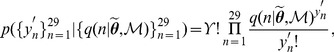 |
(31) |
where  is the total number of counts (cf. (22)).
In order to obtain  values of
  drawn from
  , each
  drawn from
  is mapped to
  .
.
We used the  -statistic for the test statistic
  [35]. The
  -statistic is proportional to the Kullback-Leibler measure of distribution divergence, and is given by
| (32) |
where  , and
, and  is the expected value for
  :
:  .
.
Applying the above approach for estimating the distribution of  under a given model
  , the posterior predictive
  -values for
  were found to be 0.005 for Model 7 and 0.006 for Model 11 (with respect to the attenuated strain),
  for Model 3 and
  for Model 5 (with respect to the virulent strain). This suggests a poor fit of the models to the data.
A visual representation of the fit of data to a model  can be provided by comparing the observed count
  (the number of cells containing
  bacteria) to the distribution of
  possible count values
  obtained via (31). This visualisation is shown in Figures 9, 10, 11 and 12.
Figure 9. The observed number of cells with  bacteria (blue) compared with 95% credibility intervals (red) predicted by Model 3 with respect to the virulent strain.

Figure 10. The observed number of cells with  bacteria (blue) compared with 95% credibility intervals (red) predicted by Model 5 with respect to the virulent strain.

Figure 11. The observed number of cells with  bacteria (blue) compared with 95% credibility intervals (red) predicted by Model 7 with respect to the attenuated strain.

Figure 12. The observed number of cells with  bacteria (blue) compared with 95% credibility intervals (red) predicted by Model 11 with respect to the attenuated strain.

Discussion
The AIC is a common maximum-likelihood approach to model comparison, but nested sampling enables a Bayesian approximation of model evidence  to be computed, along with the advantages of adopting the Bayesian approach. These include integration across parameters; estimation of the posterior parameter distributions (with visualisation of parameter correlations); and estimation of the posterior predictive distributions for goodness-of-fit assessments of the models.
Under the assumptions used, the most probable models with respect to the virulent and attenuated strains of S. enterica were burst-threshold Model 3 (Poisson) and burst-rate Model 7 ( only), respectively. The next two most probable models were burst-threshold Model 5 (negative binomial) and burst-rate Model 11 (
 plus
plus  ), respectively. However, the Bayesian posterior predictive
  -values indicate that alternative models and/or a relaxation of the quasi-stationary assumption adopted by Brown et al. [24] should be considered. It may be the case that one of the candidate models is correct but the use of pooled data was detrimental.
Other assumptions of the underlying mechanistic model may also be wrong; in particular, the absence of bacterial death and the assumption that each released bacterium infects a new macrophage.
For both the attenuated and virulent strains, the data  was recorded over a number of days following infection and then pooled, with
  . If time-dependent data is to be retained and nested sampling is to be applied then a method is required to estimate the likelihood function
  , where
  and
and  is the number of cells containing
  bacteria on the
  -th day. Branching processes have been used to model a variety of biological systems [36], and we will investigate the potential of estimating
  through the use of Bellman-Harris processes to model within-host infection dynamics.
We have demonstrated that a visualisation of the marginal and joint posterior parameter distributions  is readily obtainable once model evidence
  has been estimated by nested sampling. The estimated joint posterior distributions provided a visualisation of the correlations between the parameters. Through the use of a weighted Kolomogorov-Smirnov test, we also found that the parameter sequence
  resulting from nested sampling could not be regarded as a random sample from the posterior parameter distribution
  .
.
One drawback of Algorithm 2 is that the restricted priors will converge to a single mode when a likelihood is multi-modal, and this will cause the evidence  to be underestimated. This issue can be resolved by implementing a multi-modal version of nested sampling, such as that proposed by Feroz et al. [37] for comparing cosmological models.
Supporting Information
Toy example of nested sampling.
(PDF)
Acknowledgments
We wish to thank Dr Andrew Grant and Dr Chris Coward for their helpful contributions during discussions.
Funding Statement
RD was funded by the Biotechnology and Biological Sciences Research Council (BBSRC) (grant number BB/I002189/1). TJM was funded by the Biotechnology and Biological Sciences Research Council (BBSRC) (grant number BB/I012192/1). OR was funded by the Royal Society. The funders had no role in study design, data collection and analysis, decision to publish, or preparation of the manuscript.
References
- 1.Anderson D (2008) Model based inference in the life sciences: a primer on evidence. New York, NY: Springer Science+Business Media, LLC. [Google Scholar]
- 2. Akaike H (1974) A new look at statistical model identification. IEEE Transactions on Automatic Control AU-19 195–223. [Google Scholar]
- 3.Bishop C (2006) Pattern Recognition and Machine Learning. New York: Springer. [Google Scholar]
- 4. Schwarz G (1978) Estimating the dimension of a model. Annals of Statistics 6: 461–464. [Google Scholar]
- 5. Geman S, Geman D (1984) Stochastic relaxation, Gibbs distributions, and the Bayesian restoration of images. IEEE Transactions on Pattern Analysis and Machine Intelligence 6: 721–741. [DOI] [PubMed] [Google Scholar]
- 6. Skilling J (2004) Nested sampling. AIP Conference Proceedings 735: 395–405. [Google Scholar]
- 7. Skilling J (2006) Nested sampling for general Bayesian computation. Bayesian Analysis 1 4: 833–859. [Google Scholar]
- 8. Mukherjee P, Parkinson D, Liddle A (2006) A nested sampling algorithm for cosmological model selection. Astrophysical Journal Letters 638: L51–L54. [Google Scholar]
- 9.Murray I, Ghahramani Z, Mackay D, Skilling J (2006) Nested sampling for Potts models. In: Weiss Y, Scholkopf B, Platt J, editors. Advances in Neural Information Processing Systems (NIPS) 19. Cambridge, MA: MIT Press. pp. 947–954. [Google Scholar]
- 10. Jasa T, Xiang N (2012) Nested sampling applied in Bayesian room-acoustics decay analysis. Journal of the Acoustical Society of America 132: 3251–3262. [DOI] [PubMed] [Google Scholar]
- 11. O'Neill P (2002) A tutorial introduction to Bayesian inference for stochastic epidemic models using Markov chain Monte Carlo methods. Mathematical Biosciences 180: 103–114. [DOI] [PubMed] [Google Scholar]
- 12. Charleston B, Bankowski B, Gubbins S, Chase-Topping M, Schley D, et al. (2011) Relationship between clinical signs and transmission of an infectious disease and the implications for control. Science 332: 726–729. [DOI] [PMC free article] [PubMed] [Google Scholar]
- 13. Miller M, Raberg L, Read A, Savill N (2010) Quantitative analysis of immune response and edrythropoiesis during rodent malarial infection. PLoS Computational Biology 6: e1000946. [DOI] [PMC free article] [PubMed] [Google Scholar]
- 14. Crump J, Luby S, Mintz E (2004) The global burden of typhoid fever. Bulletin of the World Health Organization 82: 346–353. [PMC free article] [PubMed] [Google Scholar]
- 15. Mulholland E, Adegbola R (2005) Bacterial infections - a major cause of death among children in Africa. New England Journal of Medicine 352: 75–77. [DOI] [PubMed] [Google Scholar]
- 16. Crump J, Mintz E (2010) Global trends in typhoid and paratyphoid fever. Clinical Infectious Diseases 50: 241–246. [DOI] [PMC free article] [PubMed] [Google Scholar]
- 17. Mastroeni P, Grant A, Restif O, Maskell D (2009) A dynamic view of the spread and intracellular distribution of Salmonella enterica. Nature Reviews Microbiology 7: 73–80. [DOI] [PubMed] [Google Scholar]
- 18. Mastroeni P, Grant A (2011) Spread of Salmonella enterica in the body during systemic infection: unravelling host and pathogen determinants. Expert Reviews in Molecular Medicine 13: e12. [DOI] [PubMed] [Google Scholar]
- 19. Richter-Dahlfors A, Buchan A, Finlay B (1997) Murine salmonellosis studied by confocal microscopy: Salmonella typhimurium resides intracellularly inside macrophages and exerts a cytotoxic effect on phagocytes in vivo. Journal of Experimental Medicine 186: 569–580. [DOI] [PMC free article] [PubMed] [Google Scholar]
- 20. Grant A, Foster G, McKinley T, Brown S, Clare S, et al. (2009) Bacterial growth rate and host factors as determinants of intracellular bacterial distributions in systemic Salmonella enterica infections. Infection and Immunity 77: 5608–5611. [DOI] [PMC free article] [PubMed] [Google Scholar]
- 21. Grant A, Morgan F, McKinley T, Foster G, Maskell D, et al. (2012) Attenuated Salmonella Typhimurium lacking the pathogenicity island-2 type 3 secretion system grow to high bacterial numbers inside phagocytes in mice. PLOS Pathogens 8: e1003070. [DOI] [PMC free article] [PubMed] [Google Scholar]
- 22. Grant A, Sheppard M, Deardon R, Brown S, Foster G, et al. (2008) Caspase-3-dependent phagocyte death during systemic Salmonella enterica serovar Typhimurium infection of mice. Immunology 125: 28–37. [DOI] [PMC free article] [PubMed] [Google Scholar]
- 23. Sheppard M, Webb C, Heath F, Mallows V, Emilianus R, et al. (2003) Dynamics of bacterial growth and distribution within the liver during Salmonella infection. Cellular Microbiology 5: 593–600. [DOI] [PubMed] [Google Scholar]
- 24. Brown S, Cornell S, Sheppard M, Grant A, Maskell D, et al. (2006) Intracellular demography and the dynamics of Salmonella enterica infections. PLoS Biology 4: e349. [DOI] [PMC free article] [PubMed] [Google Scholar]
- 25.Dudewicz E, Mishra S (1988) Modern Mathematical Statistics. New York: John Wiley. [Google Scholar]
- 26.Sivia D, Skilling J (2006) Data Analysis: A Bayesian Tutorial, 2nd edition. Oxford: Oxford University Press. [Google Scholar]
- 27.Larson H (1982) Introduction to Probability Theory and Statistical Inference, 3rd edition. New York: John Wiley. [Google Scholar]
- 28. Feroz F, Hobson M (2008) Multimodal nested sampling: an efficient and robust alternative to MCMC methods for astronomical data analysis. Monthly Notices of the Royal Astronomical Society 2: 449–463. [Google Scholar]
- 29. Chopin N, Robert C (2010) Properties of nested sampling. Biometrika 97: 741–755. [Google Scholar]
- 30. Brown S, Cornell S, Sheppard M, Grant A, Maskell D, et al. (2006) Protocol S1: Details of model constructions and statistical analyses for “Intracellular demography and the dynamics of Salmonella enterica infections”. PLoS Biology 4: e349. [DOI] [PMC free article] [PubMed] [Google Scholar]
- 31. Garcia-Perez M (1999) MPROB: computation of multinomial probabilities. Behaviour Research Methods, Instruments and Computers 31: 701–705. [DOI] [PubMed] [Google Scholar]
- 32.Ng KM (2002) A Continuation Approach for Solving Nonlinear Optimization Problems with Discrete Variables. Ph.D. thesis, Department of Management Science and Engineering, Stanford University, Stanford, CA.
- 33. Meng XL (1994) Posterior predictive p-values. The Annals of Statistics 22: 1142–1160. [Google Scholar]
- 34.Gelman A, Carlin J, Stern H, Rubin D (1995) Bayesian Data Analysis. London: Chapman & Hall. [Google Scholar]
- 35.Sokal R, Rohlf F (1995) Biometry, 3rd edition. New York: Freeman. [Google Scholar]
- 36.Kimmel M, Axelrod D (2002) Branching Processes in Biology. New York: Springer-Verlag. [Google Scholar]
- 37. Feroz F, Hobson M, Bridges M (2009) MultiNest: an efficient and robust Bayesian inference tool for cosmology and particle physics. Monthly Notices of the Royal Astronomical Society 398: 1601–1614. [Google Scholar]
Associated Data
This section collects any data citations, data availability statements, or supplementary materials included in this article.
Supplementary Materials
Toy example of nested sampling.
(PDF)