Aggregation Distributions on Cells Determined by Photobleaching Image Correlation Spectroscopy

Abstract

The organization of molecules into macromolecular (nanometer scale), supramolecular complexes (submicron-to-micron scale), and within subcellular domains, is an important architectural principle of cellular biology and biochemistry. Determining the precise nature and distribution of complexes within the cellular milieu is a challenging biophysical problem. Time-series analysis of laser scanning confocal microscopy images by image correlation spectroscopy (ICS) or fluctuation moments methods provides information on aggregation, flow, and dynamics of fluorescently tagged macromolecules. All the methods to date require a brightness standard to relate the experimental data to absolute aggregation. In this article, we show that ICS as a function of gradual photobleaching is a sensitive indicator of aggregation distribution on the submicron scale. Specifically, in photobleaching ICS, the extent of nonlinearity of the apparent cluster density as a function of bleaching is related to the size of clusters. The analysis is tested using computer simulations on model aggregate systems and then applied to an experimental determination of Aβ peptide aggregation on nerve cells. The analysis reveals time-dependent increases in Aβ1-42 peptide aggregation. Globally, the datasets could be described by a monomer-dimer-tetramer-hexamer or a monomer-dimer-trimer-pentamer model. The results demonstrate the utility of photobleaching with ICS for determining aggregation states on the supramolecular scale in intact cells without the requirement for a brightness standard.

Introduction

The organization of biomolecules into macromolecular and supramolecular complexes underpins the function of living cells. Monomers and dimers represent the simplest and smallest quaternary states of molecules. Higher-order states of organization can also ensue in the form of large oligomers, aggregates, clusters, fibrils, and amyloid structures. Oligomerization, clustering, and compartmentalization of functional biomolecules into domains within the cellular architecture also mediate a myriad of biochemical processes. Measuring the presence and distribution of these complex reactions over several spatial and temporal scales is a significant biophysical challenge.

Fluctuation spectroscopy approaches, which began as fluorescence correlation spectroscopy (FCS) (1), represent the most versatile approaches for measuring aggregation and motion of labeled macromolecules in the cellular milieu. In conventional FCS, a laser is focused to a point in solution or in a cell and fluorescence fluctuations are recorded as a function of time (2). Analysis of these fluctuations provides the mean concentration of fluorescent particles (from the zero time-lag value of the autocorrelation function) and the transport properties of the particles (from the shape and rate of decay of the autocorrelation function in time).

Image correlation spectroscopy (ICS) (3–8), image cross-correlation spectroscopy (9), spatio-temporal ICS (10), and raster-scan ICS (11,12) have proven to be useful methods for analyzing confocal laser scanning or wide-field microscope images of immobile and mobile fluorescent particles. Originally introduced as an extension of FCS, use of those techniques has enabled information on number densities, mean degree of aggregation, and dynamics (including flow, i.e., spatio-temporal ICS; and rapid diffusion, i.e., raster-scan ICS) of fluorescent molecules in biological membranes and cell surfaces from correlation analysis of confocal laser scanning images.

Determination of aggregate sizes and distributions is a challenging problem. Analysis of the amplitude information in temporal intensity fluctuations using fluorescence intensity distribution analysis (13) and photon-counting histogram (14) provides information on aggregation states of mobile particles from point measurements. Higher-order autocorrelation and moments analysis have been applied to measure aggregation states from images and resolved bimodal monomer-oligomer distributions (15). More recently, number-brightness analysis (12,13) emerged as a useful method of measuring aggregation from a time-series of confocal or wide-field images with pixel resolution. This method provides insight into the aggregate distributions of mobile molecules within an image (from an image stack) but cannot determine the aggregation state of immobile molecules. During preparation of this article, an image version of the photon-counting histogram, the spatial intensity image distribution analysis (spIDA), appeared. This method was used to measure monomer-dimer distributions of receptor molecules on the surface of cells and was applied to fixed as well as living cells (16,17).

Photobleaching methods such as fluorescence recovery after photobleaching (18,19) have enjoyed a rich history. Fluorescence recovery after photobleaching measures the return of fluorescence after bleaching a small area of a cell and provides mobility and binding information. Photobleaching by Förster resonance energy transfer (FRET) methods employing either donor (19) or acceptor photobleaching (20) infer association of donor- and acceptor-tagged molecules on the nanometer scale but generally do not provide information on the size of aggregates. We and others have championed the use of homo-FRET with photobleaching (21–24) to determine the presence of dimers and high-order oligomers of labeled molecules on cells. This method by definition only provides information on the aggregate size of molecules on the 1–10-nm range and any supramolecular aggregation on a scale > 10 nm is missed in this approach.

Here we demonstrate that the aggregate distribution of immobile molecules (molecules that are immobile on the timescale of the experiment) can be determined from a time-series of confocal laser scanning images during photobleaching. In photobleaching ICS (pbICS), the average cluster density is directly proportional to fluorescence remaining for monomers but a nonlinear function for oligomers or clusters containing two or more labeled subunits. pbICS allow improved discrimination between different models of oligomerization, aggregation, clustering, or sequestration, as defined by spatial correlation.

To test our theory, computer simulations of photobleaching experiments on model aggregates were initially examined. Then the analysis was applied to an experimental cellular model system of biological interest: beta-amyloid peptide (Aβ) aggregation and nerve cells. The pbICS data revealed progressive aggregation over time (1–24 h). Curve fitting enabled us to compare various aggregation models. The results demonstrate the utility of photobleaching with ICS approaches for determining aggregation states on the supramolecular scale in intact cells and provide a useful adjunct to other biophysical tools, such as the family of fluctuation methods, photobleaching FRET, and homo-FRET.

Materials and Methods

All Materials and Methods are contained in the Supporting Material.

Results and Discussion

Qualitative description of photobleaching image correlation spectroscopy

Image correlation spectroscopy (ICS) measures the average density of aggregates in a given region of space (5,7). This density is inversely proportional to the amplitude of the spatial autocorrelation function (see Quantitative Theory of Photobleaching Image Correlation Microscopy, below). An aggregate can be a monomer, dimer, or higher-order oligomeric species. Because of the optical diffraction limit, the cluster density measurement refers to the density of objects but not the density of molecules within the objects. The qualitative concept of pbICS is illustrated in Fig. 1. Photobleaching of the same region by repeated scanning will photochemically deplete the fluorophores on the molecular complexes.

Figure 1.

Representation of photobleaching image correlation spectroscopy (pbICS, panels A and B). (A) Monomeric dispersed fluorophores (left panel). Partial bleaching of an image leads to a loss of fluorescent-labels and a reduction in density of fluorescent entities (middle panel). Because the amplitude of the autocorrelation function is inversely proportional to concentration of clusters (cluster density), bleaching will lead to an increase in the amplitude of the autocorrelation function (right panel). (B) Clusters of fluorophores (left panel). Partial bleaching in an image leads to a loss of fluorescent labels and a reduction in the intensity per cluster, but not a large change in the density of fluorescent entities (middle panel). As a consequence, the autocorrelation amplitude will not change significantly upon partial bleaching (right panel).

For monomeric clusters (i.e., containing one label), the amount of fluorescence remaining will be proportional to the number of clusters remaining. That is, the apparent cluster density (number of clusters per area) is a linear function of the intensity remaining (number of molecules remaining). If 50% of the fluorophores are bleached, the density of clusters will be half of the original image and the autocorrelation amplitude will be twice the original amplitude. For higher-order clusters (containing a large number of molecules per cluster) a greater number of fluorophores need to be bleached before clusters are destroyed and the cluster density would be a nonlinear function of the intensity remaining. If 50% of the fluorophores are bleached, the density of aggregates will not be significantly less than the original (but the average number of fluorophores per cluster will be less), and the autocorrelation amplitude of the postbleach image will be only slightly higher than the original image.

Quantitative theory of photobleaching image correlation microscopy

In conventional ICS (8), the intensity fluctuation spatial autocorrelation function is computed from an image I(x,y) using two-dimensional fast Fourier transform algorithm. The expression for the intensity fluctuation spatial autocorrelation function is

$$g_{11}\left(\epsilon ,\eta \right)=\frac{F^{-1}\left\{F\left(I\left(x,y\right)\right)•F^{\ast }I\left(x,y\right)\right\}}{{\left(\left|I\left(x,y\right)\right|\right)}^2}-1,$$ (1)

where F represents the Fourier transform; F⁻¹ the inverse Fourier transform; F^∗ its complex conjugate; and the values ε and η are spatial lag variables.

The autocorrelation at zero-lag, g₁₁(0,0), provides the measurement of the inverse mean number of particles per beam area and is obtained by fitting the spatial autocorrelation function to a two-dimensional Gaussian function,

$$g_{11}\left(\epsilon ,\eta \right)=g_{11}\left(0,0\right)\text{exp}\left[\frac{{\epsilon }^2+{\eta }^2}{{\omega }^2}\right]+g_{\infty }.$$ (2)

In Eq. 2, g_∞ is an offset to account for long-range spatial correlations and ω is the full-width at half-maximum of the spatial autocorrelation function. For molecular-sized aggregates, ω is the point-spread function of the microscope. Heretofore, we will refer to g₁₁(0,0) as simply g(0). In applying Eq. 2 to images after partial photobleaching, all the parameters describing the Gaussian function are determined for each bleach step, leading to a photobleaching-dependent g(0), ω, and g_∞. For molecular-sized entities, the finite optical transfer function of the microscope ensures that monomers and oligomers appear as single entities in fluorescence images with a typical width of 250–350 nm. In this case, we only need to consider g(0). (The situation where aggregates are comparable or larger than the point-spread function of the microscope is not considered here.)

We now consider how ICS is related to a distribution of aggregates. Following Petersen (3) and Petersen et al. (25), for a distribution of discrete fluorescent association states (i.e., monomer, dimer, tetramer,…), the normalized autocorrelation function at zero spatial lag (g(0)) is given as the weighted average of the individual fluorescent particles,

$$g\left(0\right)=\frac{1}{V}\frac{\sum _j{\left({\epsilon }_j{Q}_j\right)}^2{c}_j}{{\left(\sum _j{\epsilon }_j{Q}_j{c}_j\right)}^2},$$ (3)

where the subscript refers to the j^th species; the sum is over all fluorescent species; V is the volume (or area) observed in the experiment; and c_j is the mean concentration of the j^th species. Assuming that the molar extinction coefficient and the quantum yield of the labeled monomer are unaffected by the number of labeled monomers per aggregate, i.e., ε_n = nε and Q_n = Q from Eq. 3, can be written as

$$g\left(0\right)=\frac{1}{V}\frac{\sum _j{\left(j\right)}^2{c}_j}{{\left(\sum _{j}j{c}_j\right)}^2}.$$ (4)

From Eq. 4, it is clear that a measurement of the autocorrelation function amplitude cannot provide the aggregate distribution without extra information. If the sample is fixed (or aggregates immobile) but partially photobleached by continuous illumination, then the concentration of the different aggregates (c_j) will not change; however, the distribution of labeled molecules within the aggregates will change. Assume that photobleaching is irreversible, that it is random, and that the rate of photobleaching of a molecule is independent of the number of molecules in the aggregate. The probability of finding a j-mer with i-labeled subunits is given by the binomial probability function,

$$P\left(i,j,p\right)=\frac{j!}{\left(j-i\right)!i!}{\left(1-p\right)}^{\left(j-i\right)}{\left(p\right)}^i,$$ (5)

where p is the probability of finding a molecule labeled, i.e., not photobleached (by way of orientation p = [mean image intensity value after bleach]/[mean image intensity value without any photobleaching]). For a monodisperse aggregate distribution with j-subunits per aggregate and a concentration of c_j, photobleaching will create a new label distribution with P(1,j,p)c_j monomers, P(2,j,p)c_j dimers, P(3,j,p) c_j trimers, etc.

Summing over each aggregate, Eq. 4 becomes

$$g\left(0,p\right)=\frac{1}{V}\frac{\sum _j\left(\sum _{i=1}^j\frac{j!}{\left(j-i\right)!i!}{\left(1-p\right)}^{\left(j-i\right)}{\left(p\right)}^i{i}^2\right)c_j}{\left(\sum _j\left(\sum _{i=1}^j\frac{j!}{\left(j-i\right)!i!}{\left(1-p\right)}^{\left(j-i\right)}{\left(p\right)}^{i}i\right)c_j^2\right)},$$ (6)

where g(0,p) is the autocorrelation function at zero lag as a function of photobleaching the sample. Equation 6 constitutes one approach for determining the aggregate distribution of samples in an image (or region thereof) by progressively photobleaching the sample and analyzing the image stacks using spatial autocorrelation techniques.

In applying Eq. 6 to real data, the distribution of fluorescent probes is the property being determined. Thus, if 100% of molecules are labeled with one fluorophore per molecule, then the distribution extracted from Eq. 6 is equal to the true molecular distribution. Incomplete labeling at the outset (caused by incomplete binding, mixing with endogenous unlabeled molecules or incomplete fluorophore maturation in the case of genetically encoded probes) will cause an underestimation of the aggregate size distribution of the molecules being labeled. For example, dimers that are 50% labeled will have two-thirds of the population with two tags per dimer and one-third with one tag per dimer. Equation 6 can still be employed in this case to extract the dimeric population. For other labeling schemes, such as antibodies, the label distribution on the antibody must be known to convert the label distribution derived from Eq. 6 into a molecular distribution.

Computer simulations of idealized aggregates

The simple model presented above is based on probability theory, which holds in the continuum limit. It is of interest to compare the theory with simulations on a number of aggregates that is more realistic. Simulations were carried out as described in Materials and Methods (see the Supporting Material) with 1000 particles to compare with the continuum result from theory and are discussed below.

The homogenous oligomer case

It is useful to consider the reciprocal of the autocorrelation function because it provides a measure of the average number of particles per beam area or apparent cluster density (CD). For homogenous distributions of monomers (j = 1) or dimers (j = 2) or tetramers (j = 4) or j-mers, CD as a function of labeling p is given by the expressions

$$\begin{array}{l}\text{Monomers:}CD\left(p\right)=c_{1}p,\\ \text{Dimers:}CD\left(p\right)=\frac{c_2}{\left(1/2p\right)+\left(1/2\right)},\\ \text{Tetramers:}CD\left(p\right)=\frac{c_4}{\left(1/4p\right)+\left(3/4\right)},\\ j\text{-}\text{Mer}:CD\left(p\right)=\frac{c_j}{\left(\frac{1}{jp}\right)+\left(1-\frac{1}{j}\right)}.\end{array}$$ (7)

Fig. 2 A (black lines) illustrates the predicted CD versus photobleaching plot for monomeric, dimer, tetramer, and octameric distributions from Eq. 6 and from the computer simulations (monomer, green; dimer, red; tetramer, blue; and octamer; pink). As expected from qualitative considerations and the equations above, the monomeric density of aggregates decreases linearly with progressive photobleaching, octameric clusters initially decrease gradually with increasing photobleaching, and there is an apparent threshold over which the cluster density falls off more markedly with photobleaching. As a guide, the CD normalized to the initial CD after 50% bleaching (or 50% labeling) for j-mers is j/(j+1). It is clear from the shapes of the distributions that the oligomeric size can be readily determined using the pbICS approach. In the limit of no noise and 1000 particles, the agreement between theory and simulation is very good, as expected.

Figure 2.

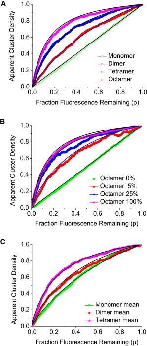
Simulations and theoretical pbICS curves as a function of cluster size. (A) Plots of the cluster density as a function of fluorescence remaining for monomer (green, j = 1), dimer (red, j = 2), tetramer (blue, j = 4), and octamer (pink, j = 8). Plots were generated from computer simulations of 1000 aggregates with fixed and homogenous aggregate sizes. (Solid curves) Plots from the continuum theory using Eq. 6 with j varied from 1 to 8 depending on oligomeric state. (B) Simulated plots of the normalized cluster density as a function of fluorescence remaining for monomer-octamer distributions. Fraction octamer increases from zero (green) to 5% (red), 25% (blue), and 100% (pink). Plots corresponding to theory (black lines) were generated with the software Excel (Microsoft, Redmond, WA) using Eq. 8 and with the normalized cluster density defined as CD(p)/CD(p = 1). (C) Simulated plots of the normalized cluster density as a function of fluorescence remaining for Poisson-distributed aggregate distributions. Mean aggregate sizes corresponding to monomers (green), dimers (red), and tetramers (blue) are shown. Plots corresponding to theory (black lines) were generated with the software Excel using Eq. 6.

The monomer-oligomer case

Complex, or polydisperse distributions (i.e., nonhomogenous), can be treated in a straightforward manner (using the result in Eq. 6 or 7) by recognizing that the autocorrelation amplitude of a mixture is the sum of the individual component autocorrelation amplitudes weighted by the square of the fractional fluorescence. In the context of the monomer-oligomer distribution, the total autocorrelation amplitude as a function of bleaching is given as the weighted sum of an oligomer contribution (g(0,p)_o and a monomer contribution (g(0,p)_m),

$$g\left(0,p\right)=\frac{g{\left(0,p\right)}_m{I}_m^2+g{\left(0,p\right)}_o{I}_o^2}{I_{\text{tot}}^2},$$ (8)

where I_m, I_o, and I_tot are the mean fluorescence intensity contributions of the monomers, oligomers, and combined populations of labeled molecules before bleaching. A simulation of monomer-octamer distributions is shown in Fig. 2 B (noting again that autocorrelation amplitude is the reciprocal of the number of particles per beam area or apparent cluster density). As expected, adding increasing fractions of octamer causes marked changes to the shapes of the pbICS profiles from theory (black lines) and simulations. Interestingly the pbICS curves were particularly sensitive to small fractions of octamers but appear to plateau in terms of sensitivity at fractions of 0.5 octamer or greater. Simulations with added noise (representing 10% of the CD value) revealed that 50:50 octamer/monomer could be distinguished from 40:60 octamer/monomer but not from 60:40 octamer/monomer, 70:30 octamer/monomer, or 90:10 octamer/monomer. The relative insensitivity to monomer fraction at moderate levels of octamer can be understood from examining the autocorrelation amplitude for mixed species. For a mixture of monomer and oligomeric states, the total autocorrelation amplitude is weighted toward the larger oligomeric species by a factor j² (3). In pbICS, the larger oligomeric species also survives j-times-more rounds of bleaching than the monomer pool.

Continuous aggregate distributions

Poisson aggregate distributions are represented in Fig. 2 C. Monomer, dimer, and tetramer Poisson distributions are shown. As expected, plots derived from Poisson distributions with average aggregate size j display increased curvature compared with homogenous models with aggregate size j (see Fig. 2 A). We note parenthetically that Poisson aggregate distribution of average size j fits equivalently to a homogenous model of aggregate size j+1. In this situation, more information is needed to distinguish between homogenous and Poissonian models.

Effect of cluster number and noise

Fig. 3 A shows the effect of noise on the simulated pbICS curves for a homogenous tetramer distribution. It is seen that adding increasing Gaussian noise affects the shape of the pbICS curves. Up to a photobleaching fraction of 0.5, decreasing the signal/background (S/B) from 1000 to 33 does not have a large effect on pbICS curves. However, a value of S/B < 33 has an appreciable effect on the simulated pbICS curve. The effect of increasing noise is also to produce a noticeable inflection in the pbICS curve at low p values. It is clear that spurious noise decreases the slope of the CD versus p plot, and consequently increases the apparent extent of aggregation.

Figure 3.

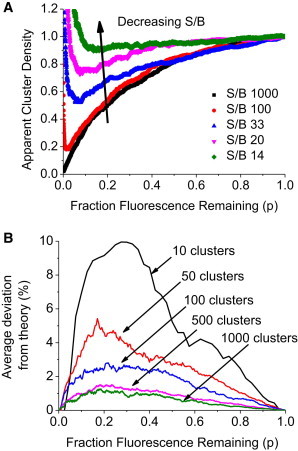
Effects of noise and finite particle number on pbICS curves. (A) Effect of increasing Gaussian noise on pbICS curves for a homogenous tetramer system. (B) Effect of finite particle number of simulated pbICS curves for homogenous tetramer. The average deviation (in %) of apparent cluster density simulation results to the analytical theory equations, Eqs. 7 and 8. The average deviation was calculated for every value of p, from 50 simulations. The effect of cluster numbers on the average deviation is clearly seen; as the cluster number increases, the average deviation decreases. This indicates a larger cluster number is preferred for accurate determination of photobleaching profile. The simulations were conducted on homogenous tetramer systems.

The effect of changing the number of clusters sampled on the pbICs profiles in shown in Fig. 3 B. The absolute average deviation from the continuum limit (Eq. 6) for tetramers is shown in the plot. For 1000 clusters sampled, the expected pbICS curve from the continuum theory agrees very well with the simulations and the deviation from theory is <2%. Decreasing the number of clusters from 1000 to 100 increases the deviation from experiment to <3% and this number increases to 10% for 10 clusters. Because of this, the accuracy of an assumed model depends on the sampling. For example, in the context of a tetramer simulation it was found that when 200 clusters were sampled, the tetramer model was adequate in 82% of cases; but for the remaining 18% of cases, either a trimer model or a pentamer model gave a better fit. At 1000 clusters, the correct model was obtained ∼95% of the time (see the Supporting Material for detailed plots).

Aβ peptide aggregation by pbICS

Alzheimer’s disease is the most common cause of dementia and is characterized by progressive memory loss, confusion, and cognitive deficits. Pathologically, this disease is primarily characterized by the presence of extracellular senile amyloid plaques, intracellular neurofibrillary tangles, cerebrovascular amyloid, and neuronal degeneration in the gray matter. The amyloid plaques are principally composed of high-order aggregates of the 39–43 residue amyloid beta (Aβ) peptide (26,27), which are derived from the amyloid precursor protein (28). While there is increasing evidence indicating that the soluble oligomeric and not the fibrillar structures are the toxic species killing the brain neurons, it is thought that the low-order oligomeric species such as the dimers or trimers (29), tetramers, or combination of oligomeric species such as the Aβ-derived diffusible ligands or amylospheroids (30) may be the most toxic species. Considering the importance of Aβ oligomerization as a key determinant of neuronal cell death, elucidating the specific oligomerization states of Aβ bound to neurons will become a valuable tool in understanding how this peptide kills brain neurons in culture, and we will be able to monitor any changes that may modulate the oligomerization profile patterns.

Primary cortical neurons were treated with carboxy fluoroscein-labeled Aβ1-42 (CF-Aβ42) peptide for defined time intervals (1, 4, and 24 h) and subsequently chemically fixed. Images of CF-Aβ42 peptide bound to primary cortical neurons were recorded using a Bio-Rad (Berkeley, CA) scanning confocal microscope (in single photon-counting mode). These images revealed the expected punctuate staining pattern of Aβ on the cell body and along the axon and dendrites of the various neurons in culture (Fig. 4). A photobleaching image series for each treatment was recorded by repetitive scanning and spatial autocorrelation analysis was performed on each image using the autocorrelation tool in the FD math function in the ImageJ software (National Institutes of Health, Bethesda, MD). Each autocorrelation image was normalized (for image size, average image intensity), corrected for background, and fit to a Gaussian function to extract the autocorrelation amplitude. Full details of the analysis and fitting procedures are outlined in the Supporting Material.

Figure 4.

Images of intact CF-Aβ42 peptide-treated neuronal cells recorded in single photon counting mode using a Bio-Rad confocal laser scanning microscope (objective 63×, laser 488 nm, FITC filter set). Primary cortical neurons were treated with CF-Aβ42 peptide for a specified time period, fixed, and mounted on a glass slide for imaging. (A) Neuronal cells treated with CF-Aβ42 showing typical punctuate staining of cell processes and cell body. (B) Neuronal cells showing diminished fluorescence intensity after a time-course photobleaching experiment. (C) Fluorescence image of a dead neuronal cell before photobleaching at 24 h after treatment. Scale bar as indicated in image.

The pbICS analysis is represented in Fig. 5 for this cellular system for data collected at 1 h (Fig. 5 A), 24 h (Fig. 5 B), and for a cell that died after prolonged exposure to the peptide (C). The normalized cluster density as a function of intensity remaining after photobleaching is plotted in Fig. 5. Inspection of the curves reveals that, in all cases, the apparent cluster density decreases monotonically with fractional fluorescence remaining with no obvious inflection points (see Fig. 3 A). This is consistent with theory and the measured S/B values of the cells (estimated to be >100). For the 1-h treated cells, the pbICS plots appear almost linear with some degree of curvature. After 24-h treatment with the peptide, the pbICS curves obtain a distinct curvature indicative of increased aggregation (Fig. 5 B). The pbICS curve of the dead cell exhibits significant curvature, suggesting even higher-order peptide aggregation. To summarize, it is clear from these pbICS plots that the shape of the apparent CD-versus-labeling curve changes with exposure time of Aβ42 to neurons in culture, suggesting increasing aggregation of the peptide over time. The changes in shape are not due to random chance because, based on the number of clusters sampled (100 ± 50 clusters), the deviations in individual datapoints are calculated to be between 3 and 5%.

Figure 5.

pbICS of a fluorescein-tagged CF-Aβ42 peptide on neuronal cells reveals progressive aggregation over time. Cells were treated with peptide for a specified time period and then fixed. (A) Apparent cluster density as a function of fluorescence remaining for cells treated with CF-Aβ42 for 1 h. (Symbols) Experimental points; (solid lines) fits to a monomer-dimer distribution of cluster sizes according to Eq. 6. (B) Apparent cluster density as a function of fluorescence remaining for cells treated with CF-Aβ42 for 24 h. (Symbols) Experimental points; (solid lines) fits to a monomer-dimer-tetramer distribution of cluster sizes according to Eq. 6. (Dashed lines) Best fit to a monomer-dimer distribution. Note the poor fit compared to the monomer-dimer-tetramer distribution. (C) Apparent cluster density as a function of fluorescence remaining for a cell treated with CF-Aβ42 for >24 h and dead at the time of fixation (rounded cell, no visible dendrites). (Symbols) Experimental points; (solid lines) fits to a monomer-dimer-tetramer-hexamer distribution of cluster sizes according to Eq. 6. (Dashed line) Best fit to a monomer-dimer-tetramer model is clearly a poorer fit than the monomer-dimer-tetramer-hexamer model.

Because the peptide contains one fluorophore per peptide, quantitative pbICS analysis can potentially reveal the actual oligomeric species involved. To get an estimate of the average extent of oligomerization, the pbICS curves were fit to a homogenous oligomerization model characterized by the single variable, j (Eq. 7) (fits nor shown). Neurons fixed after 1-h treatment were characterized with an average cluster size j = 1.2 (range of j: 0.9–1.84). For two of these cells, a monomer model was adequate to describe the data. This cluster size value increased to j = 1.7 (range of j: 1.0–3.7) after 4 h and then to j = 2 (range of N: 1.2–2.9), after 24 h. This is quantitative evidence for time-dependent aggregation of the peptide. Importantly, for many of the individual curve fits, the variable j was noninteger. The occurrence of noninteger j from these fits is nonphysical (e.g., one cannot have an oligomer with 2.5 monomers), but implies some heterogeneity in the aggregation states of the peptide in the individual cells. Therefore, in the second round of fitting, we sought the minimal aggregation model or models that could account for the data collected over the entire 24-h period. This was rationalized on the basis that the aggregation was observed to be time-dependent.

A summary of the models tested is shown in Table 1, together with the sum of least-squares. Monomer-dimer aggregation model could account for all the datasets collected at the 1-h period (examples and fits are shown in Fig. 5 A) but could not account for all data collected at 4 h (data not shown) and 24 h. An example of a fit to data collected at 4 h is shown in Fig. 5 B. All of the curves could be fit to either a monomer-dimer-tetramer (solid lines, Fig. 5 B) or a monomer-dimer-trimer model (fits not shown). However, as shown for the dashed line in Fig. 5 B, a monomer-dimer model could not fit this dataset. The situation for cells that were dead after prolonged exposure to Aβ42 before fixation, was different. These cells were readily identified as rounded, devoid of dendrites, and with high fluorescence intensity levels that did not display the staining pattern typically seen in healthier cells (Fig. 4 C).

Table 1.

Models for beta-amyloid peptide (β42) aggregation

Model/dataset	1 h	4 h	24 h	>24 h
Monomer-dimer	Yes (0.001)	No (0.3)	No (0.1)	No (0.1)
Monomer-dimer-trimer	Yes (0.001)	Yes (0.02)	Yes (0.06)	No (0.06)
Monomer-dimer-tetramer	Yes (0.001)	Yes (0.02)	Yes (0.06)	No (0.03)
Monomer-dimer-tetramer-hexamer	Yes (0.001)	Yes (0.02)	Yes (0.06)	Yes (0.009)
Monomer-dimer-trimer-pentamer	Yes (0.001)	Yes (0.02)	Yes (0.06)	Yes (0.013)

Models for amyloid β-peptide (1–42) aggregation on cultured cortical neurons. The model indicates the aggregation distribution considered in fitting the pbICS data. A model was considered adequate, indicated by Yes, when it gave the minimal sum of least-squares between experiment and theory. A model was considered inadequate, indicated with No, when it did not give the minimum sum of least-squares between experiment and theory. Sum of least-squares are indicated in the parentheses.

The apparent CD-versus-labeling curve for the dead cells had a much smaller slope near p = 1, indicating qualitatively a larger proportion of bigger aggregates in this cell (Fig. 5 C). Analysis according to the monomer-dimer-tetramer (or trimer) model was inadequate for these cells; however, inclusion of a pentamer or hexamer led to greatly improved fits. Adding even higher-order oligomers, such as octamers or dodecamers, did not significantly improve the fit quality. Taken together, the data are consistent with monomer-dimer-tetramer-hexamer or monomer-dimer-trimer-pentamer models with aggregation to the higher-order oligomers occurring at later times. We note that because of the large number of variables it was not possible to distinguish between monomer-dimer-tetramer-hexamer or monomer-dimer-trimer-pentamer models using the least-squared analysis approach.

We considered alternative means to improve distinction between models. The least-squared analysis implicitly assumes that the experimental variance in data points is a constant. An alternative approach would be to include experimental error into the data fitting and use a precision-weighted fit procedure such as χ² minimization. Because the photobleaching approach is irreversible it is not possible to estimate errors in individual data points from experiment. However, the simulations reveal that the largest deviations from theory occur with increasing extent of photobleaching (Fig. 3 B). Therefore, we took the dataset in Fig. 5 C and included a bleaching-dependent error (assumed to be linear) into a χ² minimization procedure. With an assumed maximum standard deviation of 15% of the cluster density value (corresponding to 12% deviation at p = 0.2; see Fig. 3 B), a reduced χ² value of 1.1 was obtained assuming a monomer-dimer-tetramer-hexamer model. The monomer-dimer-trimer-pentamer model recovered a slightly larger reducedχ² of 1.4 for the dataset in Fig. 5 C. Constraint of the initial cluster density value to the measured value in the fitting procedure improved the discrimination between the two models further (χ² monomer, …, hexamer = 1.28; χ² monomer, …, pentamer = 2.45).

Although further work is clearly needed to define the aggregation process, the results from the pbICS analysis are consistent with and complimentary to other analyses using very different biophysical (FRET (31), FCS (32,33), and biochemical approaches (mass spectrometry ((34)). In the cited FCS studies, it was concluded that the Aβ peptide was predominantly monomeric and/or in small oligomers in the extracellular medium, but decreased in lateral movement due to cell-membrane binding and further oligomerization. These conclusions are in good agreement with our pbICS approach on neuronal cells where we observed time-dependent increases in aggregation. Recent mass spectrometry approaches have also revealed the oligomeric intermediates in Aβ aggregation for the Ab40 peptide and the Aβ42 peptide in solution. For the Aβ42 peptide, a monomer-dimer-tetramer-hexamer-dodecamer model could account for the data in solution (34). Although we could detect the reported lower-order oligomeric intermediates in cultured neuronal cells (monomers to hexamers), our data could be modeled without the need for a large fraction of dodecameric or higher-order species. We suggest that these higher-order species possibly form later in the cells under our experimental conditions.

The results of the study of Aβ42 peptide on cultured neuronal cells reveal that the aggregation states are heterogenous and complex. Aggregation varies from cell to cell and depends on treatment time.

Disadvantages and advantages of pbICS

It is important to discuss the advantages and disadvantages of the pbICS. The photobleaching ICS method relies on varying the proportion of labeled molecules through gradual photochemical depletion of chromophores. Like other methods employing photobleaching, pbICS could be toxic to living cells and the generation of reactive oxygen can perturb biochemical and physiological function. Moreover, motions of macromolecules in living cells will invalidate the assumptions in the simple theory presented here. For these reasons, such method is recommended for fixed cells. The resolution of ICS depends on the point-spread function of the microscope and the spatial scale of spatial correlations. spIDA and N and B analyses, in contrast, are not biased by spatial correlations but instead infer aggregation from the amplitudes of temporal image fluctuations at the resolution of single pixels (N and B analysis) or from the histogram of fluorescence intensities in an image (spIDA). However, pbICS provides complementary information about spatially correlated interactions that have relevance at the subcellular and supramolecular lengthscales.

We have shown by simulation the limitations of the pbICS method. Because ICS is an imaging technique, it is possible to sample hundreds of clusters in an experiment. Under this condition and favorable S/B, the pbICS curves should reflect the underlying aggregate distribution. However, poor sampling or poor S/B can lead to significant distortions to pbICS curves.

The fitting of pbICS curves should be performed in a systematic way (e.g., global analysis) or where possible in complement to other information. This is because a single complex pbICS curve may be fit to many models, provided the models contain enough variables.

The key advantage of the pbICS method is that separate preparations of different labeled samples are not needed. For the autocorrelation analysis, photobleaching automatically generates a label distribution that can be analyzed retrospectively over an arbitrary region or regions of interest. No brightness standards are needed to obtain quantitative information about the average degree of aggregation or aggregation distributions. This is a distinct advantage of this method. In contrast, in the other cited approaches a reference standard is required to relate the data to absolute aggregation. We note also that as photobleaching homo-FRET is used to obtain aggregation information on the nanoscale, combining with pbICS will enable the aggregation and clustering of single-labeled molecules to be determined on multiple lengthscales.

References

- 1.Digman M.A., Gratton E. Lessons in fluctuation correlation spectroscopy. Annu. Rev. Phys. Chem. 2011;62:645–668. doi: 10.1146/annurev-physchem-032210-103424. [DOI] [PMC free article] [PubMed] [Google Scholar]
- 2.Magde D., Elson E.L., Webb W.W. Fluorescence correlation spectroscopy. II. An experimental realization. Biopolymers. 1974;13:29–61. doi: 10.1002/bip.1974.360130103. [DOI] [PubMed] [Google Scholar]
- 3.Petersen N.O. Scanning fluorescence correlation spectroscopy. I. Theory and simulation of aggregation measurements. Biophys. J. 1986;49:809–815. doi: 10.1016/S0006-3495(86)83709-2. [DOI] [PMC free article] [PubMed] [Google Scholar]
- 4.St-Pierre P.R., Petersen N.O. Relative ligand binding to small or large aggregates measured by scanning correlation spectroscopy. Biophys. J. 1990;58:503–511. doi: 10.1016/S0006-3495(90)82395-X. [DOI] [PMC free article] [PubMed] [Google Scholar]
- 5.Petersen N.O., Höddelius P.L., Magnusson K.E. Quantitation of membrane receptor distributions by image correlation spectroscopy: concept and application. Biophys. J. 1993;65:1135–1146. doi: 10.1016/S0006-3495(93)81173-1. [DOI] [PMC free article] [PubMed] [Google Scholar]
- 6.Wiseman P.W., Petersen N.O. Image correlation spectroscopy. II. Optimization for ultrasensitive detection of preexisting platelet-derived growth factor-β receptor oligomers on intact cells. Biophys. J. 1999;76:963–977. doi: 10.1016/S0006-3495(99)77260-7. [DOI] [PMC free article] [PubMed] [Google Scholar]
- 7.Petersen N.O., Brown C., Wiseman P.W. Analysis of membrane protein cluster densities and sizes in situ by image correlation spectroscopy. Faraday Discuss. 1998;111:289–305. doi: 10.1039/a806677i. [DOI] [PubMed] [Google Scholar]
- 8.Costantino S., Comeau J.W., Wiseman P.W. Accuracy and dynamic range of spatial image correlation and cross-correlation spectroscopy. Biophys. J. 2005;89:1251–1260. doi: 10.1529/biophysj.104.057364. [DOI] [PMC free article] [PubMed] [Google Scholar]
- 9.Comeau J.W., Kolin D.L., Wiseman P.W. Accurate measurements of protein interactions in cells via improved spatial image cross-correlation spectroscopy. Mol. Biosyst. 2008;4:672–685. doi: 10.1039/b719826d. [DOI] [PubMed] [Google Scholar]
- 10.Hebert B., Costantino S., Wiseman P.W. Spatiotemporal image correlation spectroscopy (STICS) theory, verification, and application to protein velocity mapping in living CHO cells. Biophys. J. 2005;88:3601–3614. doi: 10.1529/biophysj.104.054874. [DOI] [PMC free article] [PubMed] [Google Scholar]
- 11.Digman M.A., Sengupta P., Gratton E. Fluctuation correlation spectroscopy with a laser-scanning microscope: exploiting the hidden time structure. Biophys. J. 2005;88:L33–L36. doi: 10.1529/biophysj.105.061788. [DOI] [PMC free article] [PubMed] [Google Scholar]
- 12.Unruh J.R., Gratton E. Analysis of molecular concentration and brightness from fluorescence fluctuation data with an electron multiplied CCD camera. Biophys. J. 2008;95:5385–5398. doi: 10.1529/biophysj.108.130310. [DOI] [PMC free article] [PubMed] [Google Scholar]
- 13.Kask P., Palo K., Gall K. Fluorescence-intensity distribution analysis and its application in biomolecular detection technology. Proc. Natl. Acad. Sci. USA. 1999;96:13756–13761. doi: 10.1073/pnas.96.24.13756. [DOI] [PMC free article] [PubMed] [Google Scholar]
- 14.Chen Y., Müller J.D., Gratton E. The photon counting histogram in fluorescence fluctuation spectroscopy. Biophys. J. 1999;77:553–567. doi: 10.1016/S0006-3495(99)76912-2. [DOI] [PMC free article] [PubMed] [Google Scholar]
- 15.Sergeev M., Costantino S., Wiseman P.W. Measurement of monomer-oligomer distributions via fluorescence moment image analysis. Biophys. J. 2006;91:3884–3896. doi: 10.1529/biophysj.106.091181. [DOI] [PMC free article] [PubMed] [Google Scholar]
- 16.Swift J.L., Godin A.G., Beaulieu J.M. Quantification of receptor tyrosine kinase transactivation through direct dimerization and surface density measurements in single cells. Proc. Natl. Acad. Sci. USA. 2011;108:7016–7021. doi: 10.1073/pnas.1018280108. [DOI] [PMC free article] [PubMed] [Google Scholar]
- 17.Godin A.G., Costantino S., Wiseman P.W. Revealing protein oligomerization and densities in situ using spatial intensity distribution analysis. Proc. Natl. Acad. Sci. USA. 2011;108:7010–7015. doi: 10.1073/pnas.1018658108. [DOI] [PMC free article] [PubMed] [Google Scholar]
- 18.Jacobson K., Derzko Z., Poste G. Measurement of the lateral mobility of cell surface components in single, living cells by fluorescence recovery after photobleaching. J. Supramol. Struct. 1976;5:565–576. doi: 10.1002/jss.400050411. [DOI] [PubMed] [Google Scholar]
- 19.Jürgens L., Arndt-Jovin D., Jovin T.M. Proximity relationships between the type I receptor for Fc epsilon (FcεRI) and the mast cell function-associated antigen (MAFA) studied by donor photobleaching fluorescence resonance energy transfer microscopy. Eur. J. Immunol. 1996;26:84–91. doi: 10.1002/eji.1830260113. [DOI] [PubMed] [Google Scholar]
- 20.Wouters F.S., Bastiaens P.I., Jovin T.M. FRET microscopy demonstrates molecular association of non-specific lipid transfer protein (nsL-TP) with fatty acid oxidation enzymes in peroxisomes. EMBO J. 1998;17:7179–7189. doi: 10.1093/emboj/17.24.7179. [DOI] [PMC free article] [PubMed] [Google Scholar]
- 21.Varma R., Mayor S. GPI-anchored proteins are organized in submicron domains at the cell surface. Nature. 1998;394:798–801. doi: 10.1038/29563. [DOI] [PubMed] [Google Scholar]
- 22.Sharma P., Varma R., Mayor S. Nanoscale organization of multiple GPI-anchored proteins in living cell membranes. Cell. 2004;116:577–589. doi: 10.1016/s0092-8674(04)00167-9. [DOI] [PubMed] [Google Scholar]
- 23.Yeow E.K., Clayton A.H. Enumeration of oligomerization states of membrane proteins in living cells by homo-FRET spectroscopy and microscopy: theory and application. Biophys. J. 2007;92:3098–3104. doi: 10.1529/biophysj.106.099424. [DOI] [PMC free article] [PubMed] [Google Scholar]
- 24.Bader A.N., Hofman E.G., Gerritsen H.C. Homo-FRET imaging enables quantification of protein cluster sizes with subcellular resolution. Biophys. J. 2009;97:2613–2622. doi: 10.1016/j.bpj.2009.07.059. [DOI] [PMC free article] [PubMed] [Google Scholar]
- 25.Petersen N.O., Johnson D.C., Schlesinger M.J. Scanning fluorescence correlation spectroscopy. II. Application to virus glycoprotein aggregation. Biophys. J. 1986;49:817–820. doi: 10.1016/S0006-3495(86)83710-9. [DOI] [PMC free article] [PubMed] [Google Scholar]
- 26.Masters C.L., Multhaup G., Beyreuther K. Neuronal origin of a cerebral amyloid: neurofibrillary tangles of Alzheimer’s disease contain the same protein as the amyloid of plaque cores and blood vessels. EMBO J. 1985;4:2757–2763. doi: 10.1002/j.1460-2075.1985.tb04000.x. [DOI] [PMC free article] [PubMed] [Google Scholar]
- 27.Glenner G.G., Wong C.W. Alzheimer’s disease and Down’s syndrome: sharing of a unique cerebrovascular amyloid fibril protein. Biochem. Biophys. Res. Commun. 1984;122:1131–1135. doi: 10.1016/0006-291x(84)91209-9. [DOI] [PubMed] [Google Scholar]
- 28.Kang J., Lemaire H.G., Müller-Hill B. The precursor of Alzheimer’s disease amyloid A4 protein resembles a cell-surface receptor. Nature. 1987;325:733–736. doi: 10.1038/325733a0. [DOI] [PubMed] [Google Scholar]
- 29.Walsh D.M., Klyubin I., Selkoe D.J. Naturally secreted oligomers of amyloid β protein potently inhibit hippocampal long-term potentiation in vivo. Nature. 2002;416:535–539. doi: 10.1038/416535a. [DOI] [PubMed] [Google Scholar]
- 30.Matsumura S., Shinoda K., Hoshi M. Two distinct amyloid beta-protein (Aβ) assembly pathways leading to oligomers and fibrils identified by combined fluorescence correlation spectroscopy, morphology, and toxicity analyses. J. Biol. Chem. 2011;286:11555–11562. doi: 10.1074/jbc.M110.181313. [DOI] [PMC free article] [PubMed] [Google Scholar]
- 31.Bateman D.A., Chakrabartty A. Two distinct conformations of Aβ aggregates on the surface of living PC12 cells. Biophys. J. 2009;96:4260–4267. doi: 10.1016/j.bpj.2009.01.056. [DOI] [PMC free article] [PubMed] [Google Scholar]
- 32.Nag S., Chen J., Maiti S. Measurement of the attachment and assembly of small amyloid-β oligomers on live cell membranes at physiological concentrations using single-molecule tools. Biophys. J. 2010;99:1969–1975. doi: 10.1016/j.bpj.2010.07.020. [DOI] [PMC free article] [PubMed] [Google Scholar]
- 33.Hossain S., Grande M., Pramanik A. Binding of the Alzheimer amyloid β-peptide to neuronal cell membranes by fluorescence correlation spectroscopy. Exp. Mol. Pathol. 2007;82:169–174. doi: 10.1016/j.yexmp.2007.01.008. [DOI] [PubMed] [Google Scholar]
- 34.Bernstein S.L., Dupuis N.F., Bowers M.T. Amyloid-β protein oligomerization and the importance of tetramers and dodecamers in the etiology of Alzheimer’s disease. Nat. Chem. 2009;1:326–331. doi: 10.1038/nchem.247. [DOI] [PMC free article] [PubMed] [Google Scholar]
Associated Data
This section collects any data citations, data availability statements, or supplementary materials included in this article.