

Abstract
Purpose
The measurement of velocities based on PC-MRI can be subject to different phase offset errors which can affect the accuracy of velocity data. The purpose of this study was to determine the impact of these inaccuracies and to evaluate different correction strategies on 3D visualization.
Methods
PC-MRI was performed on a 3 T system (Siemens Trio) for in vitro (curved/straight tube models; venc: 0.3 m/s) and in vivo (aorta/intracranial vasculature; venc: 1.5/0.4 m/s) data. For comparison of the impact of different magnetic field gradient designs, in vitro data was additionally acquired on a wide bore 1.5 T system (Siemens Espree). Different correction methods were applied to correct for eddy currents, Maxwell terms and gradient field inhomogeneities.
Results
The application of phase offset correction methods lead to an improvement of 3D particle trace visualization and count. The most pronounced differences were found for in vivo/in vitro data (68%/82% more particle traces) acquired with a low venc (0.3 m/s/0.4 m/s, respectively). In vivo data acquired with high venc (1.5 m/s) showed noticeable but only minor improvement.
Conclusion
This study suggests that the correction of phase offset errors can be important for a more reliable visualization of particle traces but is strongly dependent on the velocity sensitivity, object geometry, and gradient coil design.
Keywords: phase offset errors, eddy currents, Maxwell terms, gradient inhomogeneity, 3D visualization
Introduction
Phase contrast MRI (PC-MRI) is widely used to assess blood flow. In recent years, the application of time-resolved (CINE) 3D PC-MRI (1) with three-directional velocity encoding (also termed 4D flow MRI) has gained increased interest for the evaluation of 3D hemodynamics in entire vascular structures (2,3). In this context, 3D visualization of CINE PC-MRI plays an important role in the analysis of flow characteristics inside the vessels of interest (4). Application in clinical studies requires high accuracy of 3D streamlines and time-resolved pathlines which are typically used to visualize the underlying flow information. PC-MRI relies on the measurement of changes in the signal phase due to flow or motion in the presence of known linear magnetic gradient fields. It is well know that phase offset errors due to gradient field distortions are caused by three major effects: eddy currents (5,6), concomitant gradients (Maxwell terms) (7), and gradient field distortions (non-ideal gradient coil design) (8).
All three effects can produce inaccuracies in the measured three-directional velocities (Vx, Vy, Vz) and thus result in distortion of streamlines and pathlines which may lead to incorrect visualization of flow characteristics. Although the theory and consequences of gradient field distortions are well understood, no detailed analysis of their effect on 3D visualization, derived from 4D flow MRI data, has been presented to date. In traditional 2D PC-MRI, these errors can be limited by measuring flow in vessel segments at or near the iso-center of the magnet. However, this is no longer feasible for 3D PC-MRI acquisitions with large anatomic coverage, and even small systematic inaccuracies may propagate into larger visualization errors with increasing distance from the iso-center.
It is therefore the aim of this study to systematically investigate the influence of eddy currents, Maxwell terms and gradient inhomogeneities on 3D PC-MRI data and to quantify their effect on the 3D visualization of blood flow. Experiments included in vitro data acquired on MR systems with different magnetic field gradient designs (wide versus normal bore) using different flow phantoms representing simplified geometries, such as straight and curved tubes. Additionally, the impact of PC inaccuracies on in vivo 3D flow visualization was investigated in different vascular beds (aorta, intracranial vasculature) in healthy volunteers.
Theory
As mentioned previously, three major sources of inaccuracy in velocity images include eddy current effects, Maxwell terms and gradient field non-linearities.
Eddy currents are created by rapid switching of the velocity encoding gradient. The switching results in changes of the magnetic flux-inducing currents in the conducting parts of the MR-scanner including the three gradient coils. Alterations of the desired gradient strength and duration result in spatially varying phase errors in MR images, which cause additional magnetic fields opposing the original inducing field, B0, and result as a linear or higher order velocity shift over the entire image (5,9). There is no detailed description of the distribution of the baseline shift generated by eddy currents in phase images. However, eddy currents are not purely linear (5,9). We assume that they are linear close to the iso-center and become more non-linear with increasing distance from the iso-center.
Another common inaccuracy in PC-MRI imaging is related to concomitant gradient terms, which are also known as Maxwell terms, as they are a consequence of the Maxwell equation for the divergence and curl of a magnetic field (7). It can be shown that, using Maxwell's equations, a magnetic field gradient always generates additional non-linear spatially dependent magnetic fields, and these fields produce phase errors which affect the velocity measurements using PC-MRI.
Additionally, the finite geometry constraint of the x-, y-, and z-gradients coils limits the ability to produce truly accurate fields and results in a spatially inhomogeneous distribution. These non-linear imperfections introduce errors in velocity measurements by affecting the first moments used to encode flow or motion. Any change in direction and amplitude from the ideal local gradient is directly reflected in a similar change of the first order gradient moments and thus the velocity encoding (8,10).
All three phase offset errors are strongly dependent on position within the scanner, coupled with a non-linear increase with distance from the iso-center.
Material and Methods
All experiments were performed on 3 T and 1.5 T systems (Siemens Trio and Espree, respectively, Erlangen, Germany) using a time-resolved 4D flow PC-MRI pulse sequence with three-directional velocity encoding. The two different scanners were used to investigate the impact of different magnetic field gradient designs (short bore versus long bore) on different phase offset errors.
MR Imaging – in vitro experiments
For in vitro flow experiments, a straight tube and a curved tube with an angle of 90° were integrated into a flow circuit using a flow pump (MEDOS Medizintechnik AG, Germany) that generated a constant flow of 5.3 l/min. The length of the tubes was selected to be greater than one meter to ensure laminar flow within the imaging field of view. The inner diameter was 33.5 mm (figure 1). Furthermore, a static phantom was placed next to the tubes to simulate static tissue. A fluid mimicking blood (60% water, 40% glycerol) was used to imitate blood properties (viscosity: 0.003 kg/(m*s); density: 1100 kg/m3) and contrast agent (Magnevist® 0.5 mmol/ml) was added to increase SNR. A concentration of 1.08 mmol/l was required to obtain optimal signal intensity.
Figure 1.
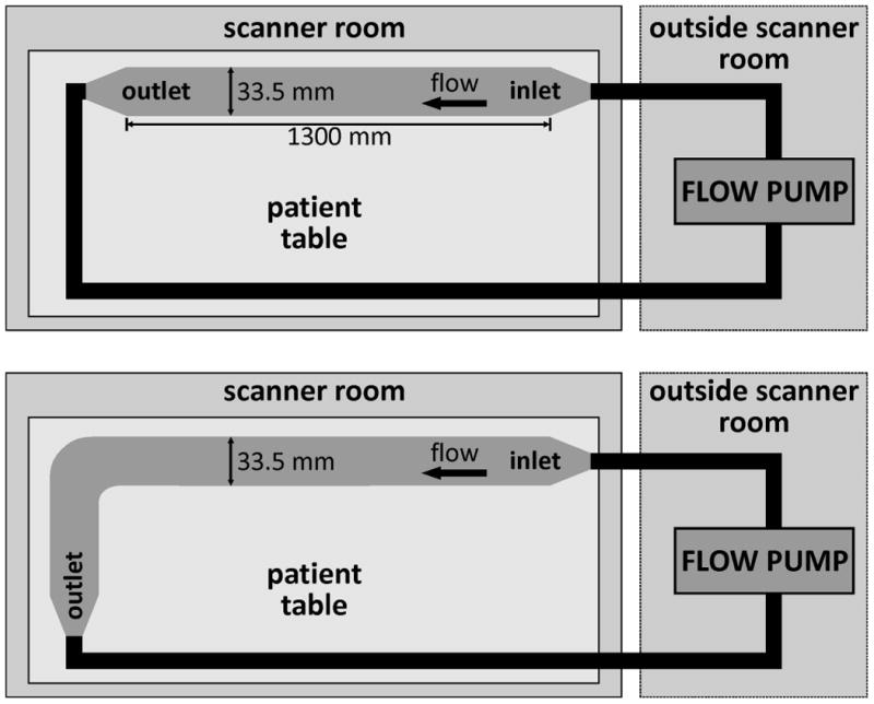
Experimental setup for the in vitro measurements for the straight (top) and the curved tube (bottom). The length of the tubes was chosen to be larger than 1 m in order to avoid the development of strong turbulences within the tubes. The pump generating stationary flow (approximately 5.3 l/min) was located outside the scanner room.
The imaging parameters for the 1.5 T and 3 T systems were set as follows: velocity encoding (venc): 0.3 m/s / 0.3 m/s, spatial resolution: 1.04×1.04×1.00 mm3 / 1.04×1.04×1.00 mm3, field of view: 300×300 mm2 / 300×300 mm2, slices: 72 / 88, flip angle: 15° / 15°, and TE: 4.5 ms / 3.7 ms. For all acquisitions the minimum TE was used based on the gradient system performance at the 1.5T and 3T systems, respectively.
To isolate the background effects, additional measurements with the flow turned off, but with otherwise identical conditions, were performed for all experiments (in vitro ‘flow-off’ data). To avoid fluid motion within the tubes or the phantom during flow-off scans, the time between flow on and flow off scans was set to approximately 5 minutes.
MR Imaging – in vivo experiments
The study was approved by our ethics board and informed consent was obtained from all participants prior to each measurement. 3D CINE PC-MRI was applied in two healthy subjects (both female and 30 years of age) to measure 3-directional blood flow velocities in different vascular territories. The thoracic aorta and the intracranial vasculature were chosen to test the influence of different velocity sensitivities (i.e., amplitude of the velocity encoding gradients) on 3D visualization inaccuracies. The imaging parameters for the aorta and the intracranial vasculature in vivo experiments were as follows: venc: 1.5 / 0.4 m/s; spatial resolution: 2.0 × 1.7 × 2.2 / 1.4 × 1.1 × 1.1 mm3; field of view: 320 × 240 / 220 × 206 mm2. As demonstrated by Chernobelsky et al. (9), a method similar to the in vitro experiments can be performed for in vivo data to isolate the background effects. Measurements of the thoracic aorta were thus repeated using the same sequence parameters, by placing a stationary phantom (water bottle, in vivo ‘flow off’ data) at the position of the thoracic aorta on the scanner patient table. To retain the scanner table coordinates, and therefore the same FOV and slice position, the table was removed from the scanner bore but stopped before the position where scanner coordinates are cleared. This left enough space for the volunteer to leave the patients table. Phantom measurements for the subtraction method were only performed in the aorta.
Data Analysis - Corrections
All corrections were performed using home-built software tools programmed in MATLAB (Mathworks, Natick, MA, USA).
Eddy currents
Determination of static regions and tissue. This was accomplished in vitro by manually selecting a region of interest in the static phantom, for each slice and in vivo, and defining a threshold based separation of regions with static tissue from blood flow and noise by using the velocity-time standard deviation for each pixel. Pixels were regarded as static tissue for standard deviations below the adjusted threshold (5,11,12).
Fitting a plane (1st order / 2nd order) with least squares method to the static regions of the single time frame for stationary flow data (in vitro) or the last time frame (late diastole) for time resolved data (in vivo). The plane was fitted to the last diastolic time frame to ensure minimal blood flow.
Applying the correction by subtraction of the fitted surface from the PC-MRI data in the single time frame (in vitro) or for all time frames (in vivo)(13,14).
Maxwell Terms and eddy currents
For the simultaneous correction of both Maxwell terms and eddy currents, flow-on data was subtracted from the flow-off measurements for in vivo and in vitro measurements. This approach was based on the assumption that eddy current induced phase shifts and Maxwell terms remain constant for the same imaging parameters.
Gradient Field Non-Linearities
The true magnitude and direction of the underlying velocities can be recovered from the phase difference images by a generalized phase contrast velocity reconstruction which requires the measurement of full three-directional velocity information as reported previously (8). Briefly, after 3D distortion correction (calculated by the scanner software), the effects of gradient field inhomogeneities on phase contrast data were corrected by calculating the relative field deviations based on an MR-system specific gradient field model (spherical harmonic expansion) for x-, y-, and z gradient coils (15). To account for the deviation of the ideal gradient field (spatially constant) from the actual (modeled) field strength, relative field deviations are introduced. These relative field deviations describe the relative error in the first moments and therefore the encoded velocity induced phase shift in phase contrast MRI. Based on the knowledge of the relative field deviations the undistorted velocities can be recovered for the measured velocity data. For further details see Markl et al. (8).
Data Analysis
After phase-offset corrections, all data were loaded into a 3D visualization program (EnSight, CEI, NC, USA). 3D flow characteristics were visualized using streamlines for in vitro data with steady flow and time-resolved pathlines over the cardiac cycle for in vivo data with pulsatile flow. Additionally a particle trace count was performed to quantify the number of streamlines and pathlines reaching a certain target plane for the different correction methods.
Furthermore, the distribution of these traces within the tube/vessel was analyzed. Therefore we separated the particle trace count in the target plane into four quadrants. In an ideal case without phase offset errors, particle traces should be equally distributed over all 4 quadrants. If no particle traces were found in a quadrant this implies errors in the underlying data of particle trace calculation.
In vitro phantom data
The geometry of the flow phantoms was visualized by threshholding the signal intensity in the magnitude images. 2D analysis planes were manually positioned at the center of the phantoms as illustrated in figures 2 and 3 (dashed lines). The central plane was used to emit n=400 streamlines up- and downstream of the plane location. The resulting traces provide a visual impression of the 3D distribution and direction of the measured 3-directional flow velocities.
Figure 2.
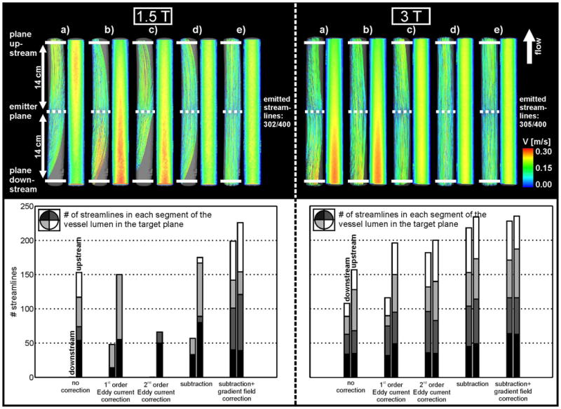
Top: Streamline visualization at 1.5 T (left) and 3 T (right) inside the straight tube for a) uncorrected data, b) first order eddy current correction, c) second order eddy current correction, d) eddy current and Maxwell correction and e) subtraction method and gradient inhomogeneity correction of phase contrast data. Streamlines originated from the emitter plane at the center of the tube (dotted line). The solid white lines indicate the planes for the streamline counts up- and downstream from the emitter plane. Bottom: Streamline count at 1.5 T (left) and 3 T (right) upstream and downstream from the emitter plane. The distribution of the streamlines in the lumen is indicated by the different gray scales.
Figure 3.
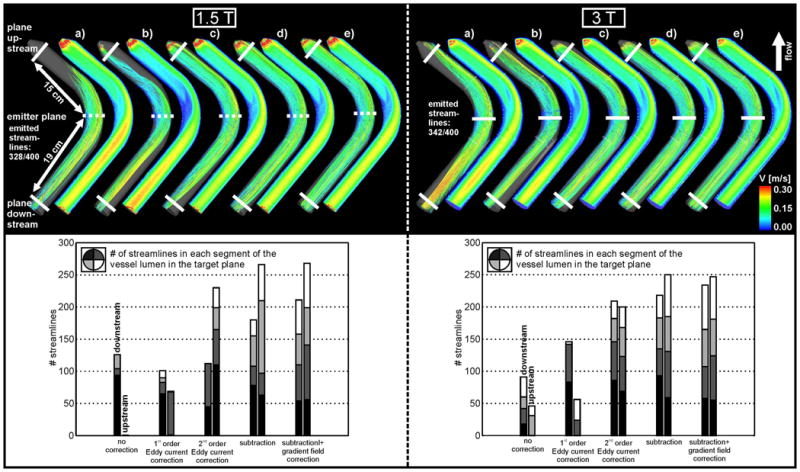
Top: Streamline visualization at 1.5 T (left) and 3 T (right) inside the curved tube for a) uncorrected data, b) first order eddy current correction, c) second order eddy current correction, d) eddy current and Maxwell correction and e) subtraction method and gradient inhomogeneity correction of phase contrast data. Bottom: Streamline count at 1.5 T (left) and 3 T (right) upstream and downstream from the emitter plane. The distribution of the streamlines in the lumen is indicated by the different gray scales in each bar, as for Figure 2.
To evaluate the effect of correction strategies, the number of streamlines reaching target planes at the inlet and outlet of the flow phantoms were determined. The more streamlines are reaching the target plane the better the correction of the phase offset errors. For the straight tube, target planes were positioned 14 cm up- and downstream from the central plane (figure 2). For the tube with the 90° angle, streamline count was performed in target planes located 15 cm upstream and 19 cm downstream from the emitter plane (figure 3).
In vivo data
For the depiction of vascular geometry, time-averaged PC MR angiography data was calculated from the 4D flow measurements as described by Bock et al. (16). For aortic 4D flow MRI, 3D blood flow visualization of pulsatile flow was based on time resolved pathlines (n=700) emitted from the mid-ascending aorta as shown in figure 4. For the intracranial vasculature, n=400 pathlines originated from the mid-sagittal sinus (figure 5). The resulting pathlines depict the trajectories that individual fluid elements follow over the cardiac cycle.
Figure 4.
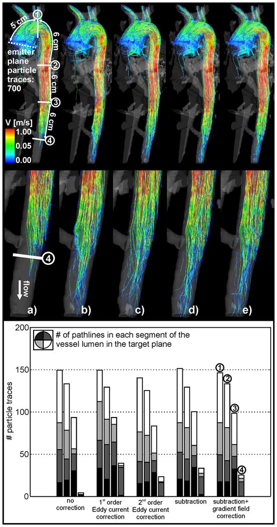
Top: Pathline visualization in the thoracic aorta for a) uncorrected data, b) first order eddy current correction, c) second order eddy current correction, d) eddy current and Maxwell correction and e) subtraction method and gradient inhomogeneity correction of phase contrast data. Pathlines originated from the emitter plane at the ascending aorta (dotted line). The four solid white lines indicate the planes for the pathline counts downstream from the emitter plane. Bottom: Pathline count downstream of the emitter plane.
Figure 5.
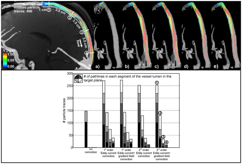
Top: Pathline visualization inside the intracranial vessel for a) uncorrected data, b) first order eddy current correction, c) second order eddy current correction, d) eddy current and Maxwell correction and e) subtraction method and gradient inhomogeneity correction of phase contrast data. Pathlines originated from the emitter plane at the proximal sagittal sinus (dotted line). The four solid white lines indicate the planes for the pathline counts downstream from the emitter plane. Bottom: Pathline count downstream of the emitter plane.
For each (aorta / intracranial vasculature) data set, a series of four target planes were positioned downstream of the emitter plane and illustrated in figures 4 and 5. For the pathline count, the target planes were additionally subdivided into 4 angular segments to quantify the intra-luminal distribution of pathlines.
The emitted streamlines/pathlines and the target plane locations were exported from the visualization software (data in a comma delimited format). The quantification of streamlines/pathlines reaching the target planes was performed using a home-built software tool programmed in MATLAB.
Results
In vitro experiments
Figures 2 and 3(top row) show the subsequent application of all correction methods which resulted in an improvement of the 3D streamline visualization when compared with those computed from the uncorrected data. As expected, the 1.5 T wide bore system showed stronger distortions in the streamline visualization than the 3 T system. Improvements in streamline visualization that could be achieved with the different correction methods are summarized in tables 1 and 2.
Table 1.
Fraction of streamlines reaching the target planes upstream/downstream from the emitter plane for the straight (left) and the curved tube (right) for the wide bore 1.5 T system. Between 64% and 82% of the emitted streamlines reached the target planes when all correction methods were applied.
| 1.5T system | straight tube | curved tube | ||
|---|---|---|---|---|
| plane # | down | up | down | up |
| no correction | 0% | 51% | 38% | 0% |
| 1st order | 16% | 50% | 31% | 21% |
| 2nd order | 0% | 22% | 34% | 70% |
| subtraction | 19% | 58% | 55% | 81% |
| sub + grad field | 66% | 75% | 64% | 82% |
Table 2.
Fraction of streamlines reaching target planes upstream/downstream from the emitter plane for the straight (left) and the curved tube (right) for the 3 T system. Between 68% and 77% of the emitted streamlines reached the target planes when all correction methods were applied.
| 3T system | straight tube | curved tube | ||
|---|---|---|---|---|
| plane # | down | up | down | up |
| no correction | 35% | 51% | 26% | 13% |
| 1st order | 38% | 64% | 43% | 16% |
| 2nd order | 60% | 66% | 61% | 58% |
| subtraction | 71% | 77% | 64% | 73% |
| sub + grad field | 75% | 77% | 68% | 72% |
The uncorrected data showed strong distortions of streamlines throughout the phantom (top row in figures 2a and 3a) for the straight and the curved tube. For the 1.5 T wide bore system the streamlines did not reach the up- and downstream target planes and the downstream plane for the curved and straight tube, respectively. The effect of PC inaccuracies is further illustrated by the cross sectional images showing strong velocity variations along the tubes which should be absent for steady flow.
1st order eddy current correction clearly improved the streamline visualization for both phantoms and for the different MR systems (figures 2b and 3b) with an increase in the streamline count of up to 17% for 3 T and 21% for the 1.5 T wide bore system (tables 1 and 2). Further improvement could be achieved with 2nd order eddy current correction for the 3 T system (45% increase in streamline count and a smoother distribution of streamlines in the tube lumen - see figure 2c, right) while the 2nd order correction was ineffective at 1.5 T (figure 2c, left, and table 1). In contrast, the curved tube showed improvements for both the 3 T and wide bore 1.5 T system.
Correction for both eddy current and Maxwell terms resulted in further improvements (up to 81% from uncorrected data). However, strong distortions of streamlines were still observed for the wide bore 1.5 T system.
The remaining distortions of the streamlines could be removed by correcting for gradient field inhomogeneities of phase contrast data. As expected, the effect was more pronounced for the wide bore 1.5 T system (figures 2e and 3e; left). For the 3 T system, only minor changes in the streamline count (approximately 4%) were observed. Nevertheless, the correction for gradient field non-linearities resulted in an improved distribution of streamlines across the tube lumen (figures 2 and 3, bottom row). It should be noted that even for a combination of all correction strategies, no more than 82% of the originally emitted streamlines reached the target planes.
In vivo experiments
The impact of the successive application of correction methods to in vivo pathline visualization is shown in figures 4 and 5. For aortic 4D flow MRI, only a minor improvement (1%) in the number of pathlines reaching the first three target planes was noticeable and an increase between 2% and 5% for the fourth target plane in the distal descending aorta was observed (table 3). However, correction for phase offset errors resulted in a more even distribution of pathlines within the vessel lumen (bar plots, figure 4b-e; bottom row).
Table 3.
Fraction of pathlines reaching the four target planes downstream along the aorta.
| Aorta | ||||
|---|---|---|---|---|
|
| ||||
| plane # | 1 | 2 | 3 | 4 |
|
| ||||
| no correction | 21% | 19% | 13% | 1% |
|
| ||||
| 1st order | 21% | 18% | 13% | 6% |
|
| ||||
| 2nd order | 20% | 18% | 12% | 3% |
|
| ||||
| subtraction | 22% | 18% | 14% | 5% |
|
| ||||
| sub + grad field | 21% | 19% | 14% | 4% |
Pathline distortions and improvements after correction were more pronounced for the intracranial venous flow with almost complete loss of pathlines before correction (figure 5a, top / bar plot, bottom row). The 1st and 2nd order eddy current correction with additional gradient field correction of phase contrast data showed clearly improved visualization of pathlines (figures 5b-e, top row) for all 4 target planes along the vessel (increase of 9% - 36%; see also table 4).
Table 4.
Fraction of pathlines reaching the four target planes downstream along the sagittal sinus.
| Head | ||||
|---|---|---|---|---|
| plane # | 1 | 2 | 3 | 4 |
| no correction | 37% | 0% | 0% | 0% |
| 1st order | 68% | 36% | 19% | 10% |
| 1st order + grad field | 68% | 36% | 15% | 9% |
| 2nd order | 63% | 32% | 10% | 3% |
| 2nd order + grad field | 63% | 33% | 9% | 3% |
Discussion
The results of this study clearly demonstrate the importance of correcting the three major sources of gradient field distortions for 3D visualization of 3-directional MR velocity data. Our study suggests that appropriate correction strategies should be applied to correct for phase offset errors and to ensure accurate particle trace visualization using 3D CINE PC-MRI data. Although these distortions are well understood, appropriate correction methods are often absent or only partly applied in the present literature. It is important to note that such phase offset errors exhibit a substantial and non-linear increase with increasing distance from the iso-center.
As indicated by the comparison of the in vivo aortic and intracranial 3D CINE PC-MRI data, correction of phase offset errors is important for measurements with small venc, e.g. for venous flow or small vessels. A substantially lower venc and thus stronger velocity encoding gradients for the in vitro models and the intracranial venous flow data resulted in increased eddy current and Maxwell effects and therefore stronger distortions of particle traces. In contrast, 3D CINE PC-MRI measurements performed in vessels at or near the iso-center of the magnet and/or using higher vencs (such as 1.5 m/s) are relatively insensitive to these errors as can be seen in the example of the thoracic aorta. Therefore, it is important to consider the velocity encoding sensitivity and the position of the vessel within the scanner as they have a strong influence on phase contrast inaccuracies.
While the majority applications of 3D CINE PC MRI focus on arterial regions with high peak flow velocities, there are a substantial number of applications that require the measurement of slower venous flow in tortures vessel geometries such as the assessment of arterial and venous hemodynamics in congenital heart disease, in the portal venous system of the liver, or the evaluation of blood flow characteristics in cerebrovascular disease (aneurysm, anterio-venous malformations, AVM). Venous velocities are typically low and thus require reduced velocity sensitivity (venc) and therefore stronger encoding gradients. As a result, eddy currents play a more important role in 3D CINE PC MRI of the venous system. In our study, the sagittal sinus superior was chosen as a test case for vascular regions with low blood flow velocities to illustrate the effect of reduced venc and thus increased encoding gradients and eddy currents. In neurovascular applications, 3D CINE PC-MRI is typical prescribed with full or partial volumetric coverage of the entire head in order to evaluate complex cerebrovascular diseases such as aneurysms or arteriovenous malformations (17-24). As a result, individual vessels such as the sagittal sinus are often not acquired at the iso-center wich enhances the effect of eddy currents as demonstrated by the results of our study.
The subtraction method as proposed by Chernobelsky et al. (9) (subtraction of subsequently acquired static phantom data from in vivo data) was able to clearly reduce streamline and pathline distortions. The remaining distortions were small and could be further corrected using the gradient field inhomogeneity correction method. Nonetheless, the subtraction method is often time consuming since it requires an additional phantom measurement with identical imaging parameters and therefore doubles the measurement time.
For in vivo data of the aorta measured at high venc, the effects of phase-offset errors in 3D visualization were small (changes in pathlines count of only up to 5%).
As expected, the gradient field inhomogeneity correction of the phase data was much more effective for the wide bore systems with shorter gradient coils and consequently increased gradient field non-linearities. Errors induced by gradient field distortions need to be corrected to ensure accurate visualization as demonstrated in this study. This is of particular importance for particle trace visualization covering a large distance from the iso-center. Small systematic inaccuracies can propagate into larger visualization errors with increasing distance from the emitter plane.
It should be note that a fraction of pathlines emitted in the ascending aorta does not reach the target plane in the descending aorta due to flow to the supra-aortic arteries. In the case presented in this study, we have estimated the loss of flow to the supra-aortic branches by calculating the difference of flow in the planes the AAo (emitter plane) as approx. 25% of the total flow in the DAo (target plane 2). However, the calculated loss of pathlines was 81 %. This big loss of pathlines between the two planes is not only due to phase offset errors. Another criterion for the abort of particle trace calculation could be a low signal to noise ratio, low velocities near the vessel wall and at the end of the cardiac cycle and a low resolution of the underlying data.
The 2nd order eddy current correction resulted in improved 3D visualization (more even distribution of particle traces within the iso-surface with up to 49% more particle traces reaching the target planes) when compared with 1st order eddy current correction. This finding indicates that either eddy currents show a stronger than expected non-linear behavior or second order Maxwell terms remained present in the data. However, for some experiments, the 2nd order eddy current correction resulted in impaired 3D visualization comparison to the 1st order correction. We speculate that the 2nd order fit to phase variation in the static region was more susceptible to local signal variation due to noise which may have led to overestimation of regional eddy current induced phase offset errors. Other reasons for the weak performance of the 2nd order eddy current correction for in vivo data could be due the incorrect separation of static tissue and regions with flow, or an insufficient size of the static tissue region to calculate an appropriate 2nd order fit. In this context, the 1st order and 2nd order fitting procedure was only performed for the last time frame. The resulting estimate of the phase offset error was then subtracted from all time frames in the cardiac cycle. Future studies should thus investigate if the application of this correction step for each time frame separately might yield increased accuracy.
Future work should also involve a systematic variation of the velocity encoding gradient to analyze its effect on particle trace visualization of in vivo and in vitro data. This study included only 2 in vivo data sets. For a statistical analysis of the effect of inaccuracies and corrections by comparing results it would be necessary to perform the correction methods on a cohort of subjects.
Conclusion
The correction of phase offset errors is necessary and important for a correct visualization of particle traces. This study illustrated a substantial improvement of particle trace visualization and count by using the applied correction methods. For experiments involving a significant distance from the iso-center and/or lower vencs, the application of phase offset error correction techniques is of substantial importance for accurate flow visualization.
Acknowledgments
JGK acknowledges support from the Excellence Inititiative of the German Federal and State governments, as well as an operating grant from the University of Freiburg.
Grant support: NIH NHLBI grant R01HL115828; NUCATS Institute NIH grant UL1RR025741, and the Northwestern Memorial Foundation Dixon Translational Research Grants Initiative
Footnotes
Parts of this work were presented at the ISMRM 2010 in Stockholm, Sweden
References
- 1.Pelc NJ, Herfkens RJ, Shimakawa A, Enzmann DR. Phase contrast cine magnetic resonance imaging. Magnetic resonance quarterly. 1991;7(4):229–254. [PubMed] [Google Scholar]
- 2.Frydrychowicz A, Harloff A, Jung B, Zaitsev M, Weigang E, Bley TA, Langer M, Hennig J, Markl M. Time-resolved, 3-dimensional magnetic resonance flow analysis at 3 T: visualization of normal and pathological aortic vascular hemodynamics. Journal of computer assisted tomography. 2007;31(1):9–15. doi: 10.1097/01.rct.0000232918.45158.c9. [DOI] [PubMed] [Google Scholar]
- 3.Wigstrom L, Ebbers T, Fyrenius A, Karlsson M, Engvall J, Wranne B, Bolger AF. Particle trace visualization of intracardiac flow using time-resolved 3D phase contrast MRI. Magn Reson Med. 1999;41(4):793–799. doi: 10.1002/(sici)1522-2594(199904)41:4<793::aid-mrm19>3.0.co;2-2. [DOI] [PubMed] [Google Scholar]
- 4.Buonocore MH. Visualizing blood flow patterns using streamlines, arrows, and particle paths. Magn Reson Med. 1998;40(2):210–226. doi: 10.1002/mrm.1910400207. [DOI] [PubMed] [Google Scholar]
- 5.Walker PG, Cranney GB, Scheidegger MB, Waseleski G, Pohost GM, Yoganathan AP. Semiautomated method for noise reduction and background phase error correction in MR phase velocity data. J Magn Reson Imaging. 1993;3(3):521–530. doi: 10.1002/jmri.1880030315. [DOI] [PubMed] [Google Scholar]
- 6.Gatehouse PD, Rolf MP, Bloch KM, Graves MJ, Kilner PJ, Firmin DN, Hofman MB. A multi-center inter-manufacturer study of the temporal stability of phase-contrast velocity mapping background offset errors. J Cardiovasc Magn Reson. 2012;14:72. doi: 10.1186/1532-429X-14-72. [DOI] [PMC free article] [PubMed] [Google Scholar]
- 7.Bernstein MA, Zhou XJ, Polzin JA, King KF, Ganin A, Pelc NJ, Glover GH. Concomitant gradient terms in phase contrast MR: analysis and correction. Magn Reson Med. 1998;39(2):300–308. doi: 10.1002/mrm.1910390218. [DOI] [PubMed] [Google Scholar]
- 8.Markl M, Bammer R, Alley MT, Elkins CJ, Draney MT, Barnett A, Moseley ME, Glover GH, Pelc NJ. Generalized reconstruction of phase contrast MRI: analysis and correction of the effect of gradient field distortions. Magn Reson Med. 2003;50(4):791–801. doi: 10.1002/mrm.10582. [DOI] [PubMed] [Google Scholar]
- 9.Chernobelsky A, Shubayev O, Comeau CR, Wolff SD. Baseline correction of phase contrast images improves quantification of blood flow in the great vessels. J Cardiovasc Magn Reson. 2007;9(4):681–685. doi: 10.1080/10976640601187588. [DOI] [PubMed] [Google Scholar]
- 10.Peeters JM, Bos C, Bakker CJ. Analysis and correction of gradient nonlinearity and B0 inhomogeneity related scaling errors in two-dimensional phase contrast flow measurements. Magn Reson Med. 2005;53(1):126–133. doi: 10.1002/mrm.20309. [DOI] [PubMed] [Google Scholar]
- 11.Caprihan A, Altobelli SA, Benitez-Read E. Flow-velocity imaging from linear regression of phase images with techniques for reducing eddy-current effects. Journal of Magnetic Resonance (1969) 1990;90(1):71–89. [Google Scholar]
- 12.Lankhaar JW, Hofman MB, Marcus JT, Zwanenburg JJ, Faes TJ, Vonk-Noordegraaf A. Correction of phase offset errors in main pulmonary artery flow quantification. J Magn Reson Imaging. 2005;22(1):73–79. doi: 10.1002/jmri.20361. [DOI] [PubMed] [Google Scholar]
- 13.Bock J, Kreher BW, Hennig J, Markl M. Optimized pre-processing of time-resolved 2D and 3D Phase Contrast MRI data. Proceedings of the 15th Scientific MeetingInternational Society for Magnetic Resonance in Medicine; Berlin, Germany. 2007. p. #3138. [Google Scholar]
- 14.Carr JC, Carroll TJ. Magnetic Resonance Angiography: Principles and Applications. Vol. 1. Springer Verlag; New York: 2012. p. 412. [Google Scholar]
- 15.Romeo F, Hoult DI. Magnet field profiling: analysis and correcting coil design. Magn Reson Med. 1984;1(1):44–65. doi: 10.1002/mrm.1910010107. [DOI] [PubMed] [Google Scholar]
- 16.Bock J, Frydrychowicz A, Stalder AF, Bley TA, Burkhardt H, Hennig J, Markl M. 4D phase contrast MRI at 3 T: effect of standard and blood-pool contrast agents on SNR, PC-MRA, and blood flow visualization. Magn Reson Med. 2010;63(2):330–338. doi: 10.1002/mrm.22199. [DOI] [PubMed] [Google Scholar]
- 17.Ansari SA, Schnell S, Carroll T, Vakil P, Hurley MC, Wu C, Carr J, Bendok BR, Batjer H, Markl M. Intracranial 4D Flow MRI: Toward Individualized Assessment of Arteriovenous Malformation Hemodynamics and Treatment-Induced Changes. Ajnr. 2013 doi: 10.3174/ajnr.A3537. [DOI] [PMC free article] [PubMed] [Google Scholar]
- 18.Bachler P, Valverde I, Pinochet N, Nordmeyer S, Kuehne T, Crelier G, Tejos C, Irarrazaval P, Beerbaum P, Uribe S. Caval blood flow distribution in patients with Fontan circulation: quantification by using particle traces from 4D flow MR imaging. Radiology. 2013;267(1):67–75. doi: 10.1148/radiol.12120778. [DOI] [PubMed] [Google Scholar]
- 19.Boussel L, Rayz V, Martin A, Acevedo-Bolton G, Lawton MT, Higashida R, Smith WS, Young WL, Saloner D. Phase-contrast magnetic resonance imaging measurements in intracranial aneurysms in vivo of flow patterns, velocity fields, and wall shear stress: comparison with computational fluid dynamics. Magn Reson Med. 2009;61(2):409–417. doi: 10.1002/mrm.21861. [DOI] [PMC free article] [PubMed] [Google Scholar]
- 20.Chang W, Loecher MW, Wu Y, Niemann DB, Ciske B, Aagaard-Kienitz B, Kecskemeti S, Johnson KM, Wieben O, Mistretta C, Turski P. Hemodynamic changes in patients with arteriovenous malformations assessed using high-resolution 3D radial phase-contrast MR angiography. Ajnr. 2012;33(8):1565–1572. doi: 10.3174/ajnr.A3010. [DOI] [PMC free article] [PubMed] [Google Scholar]
- 21.Hope MD, Purcell DD, Hope TA, von Morze C, Vigneron DB, Alley MT, Dillon WP. Complete intracranial arterial and venous blood flow evaluation with 4D flow MR imaging. Ajnr. 2009;30(2):362–366. doi: 10.3174/ajnr.A1138. [DOI] [PMC free article] [PubMed] [Google Scholar]
- 22.Markl M, Geiger J, Kilner PJ, Foll D, Stiller B, Beyersdorf F, Arnold R, Frydrychowicz A. Time-resolved three-dimensional magnetic resonance velocity mapping of cardiovascular flow paths in volunteers and patients with Fontan circulation. Eur J Cardiothorac Surg. 2011;39(2):206–212. doi: 10.1016/j.ejcts.2010.05.026. [DOI] [PubMed] [Google Scholar]
- 23.Morisaka H, Motosugi U, Ichikawa T, Sano K, Ichikawa S, Araki T, Enomoto N. MR-based Measurements of Portal Vein Flow and Liver Stiffness for Predicting Gastroesophageal Varices. Magn Reson Med Sci. 2013 doi: 10.2463/mrms.2012-0052. [DOI] [PubMed] [Google Scholar]
- 24.Stankovic Z, Csatari Z, Deibert P, Euringer W, Blanke P, Kreisel W, Abdullah Zadeh Z, Kallfass F, Langer M, Markl M. Normal and altered three-dimensional portal venous hemodynamics in patients with liver cirrhosis. Radiology. 2012;262(3):862–873. doi: 10.1148/radiol.11110127. [DOI] [PubMed] [Google Scholar]