Selecting an Appropriate Caliper Can Be Essential for Achieving Good Balance With Propensity Score Matching

Abstract

Matching on the propensity score is widely used to estimate the effect of an exposure in observational studies. However, the quality of the matches can be affected by decisions made during the matching process, particularly the order in which subjects are selected for matching and the maximum permitted difference between matched subjects (the “caliper”). This study used simulations to explore the effects of these decisions on both the imbalance of covariates and the closeness of matching, while allowing the numbers of potential matches and strengths of association between the confounding variable and the exposure to vary. It was found that, without a caliper, substantial bias was possible, particularly with a relatively small reservoir of potential matches and strong confounder-exposure association. Use of the recommended caliper reduced the bias considerably, but bias remained if subjects were selected by increasing or decreasing propensity score. A tighter caliper led to greatly reduced bias and closer matches, although some subjects could not be matched. This study suggests that a narrow caliper can improve the performance of propensity score matching. In situations where it is impossible to find appropriate matches for all exposed subjects, it is better to select subjects in order of the best available matches, rather than increasing or decreasing the propensity score.

Propensity score matching is widely used in epidemiologic observational studies to reduce bias in estimates of the effect of an exposure due to confounding by indication. For example, a systematic review by Austin (1) identified 47 articles published in the medical literature between 1996 and 2003. Matching as a statistical technique has been used since the middle of the twentieth century (2, 3), although it was given a solid theoretical basis only later (4–6). It can be difficult to find appropriate matches when trying to match on several variables, but Rosenbaum and Rubin (7) showed that matching on the propensity score (the conditional probability of exposure given a set of covariates) could produce samples with the same distribution of covariates in exposed and unexposed subjects.

In order to be able to find suitable matches for all exposed subjects, the number of controls available needs to be greater than the number of exposed subjects; the ratio typically lies in the range of 2–20, although it may be higher (8). However, if there is considerable separation between exposed and unexposed subjects on the propensity score, there may be few unexposed subjects with high propensity scores, even when there are many times more unexposed subjects than exposed subjects. Thus, there may be few, or no, suitable matches for some exposed subjects with high propensity scores.

There is little advice in the literature on the practicalities of matching, in particular, the choice of “caliper.” Rosenbaum and Rubin (9) matched on the log of the odds of being exposed (i.e., the linear predictor from the logistic regression model used to predict exposure) and used a caliper of 0.25 standard deviations based on the results of Cochran and Rubin (4), and this has been taken as a recommendation. However, Raynor (10) showed that the appropriate caliper depended on the association between the outcome variable and the matching variable; a stronger association would mean more confounding for a given difference and, hence, a tighter caliper would be more appropriate. Furthermore, the appropriate caliper depends to some extent on the data set to which it is being applied; it should be tight enough to produce close matches for efficiency, but not so tight that it becomes impossible to match a number of exposed subjects, which could introduce both inefficiency (due to the reduced sample size) and selection bias. A tight caliper would be preferred when matches are easy to find (e.g., when there is little difference between exposed and unexposed subjects, and there is a large pool of unexposed subjects from which to select) and a looser one when matches are harder. In practice, a wide variety of calipers is used (1) and, with the exception of Austin (11) (who recommended reducing the caliper from 0.25 standard deviations to 0.2 standard deviations), more recent papers on the practicalities of matching have not given recommendations for setting a caliper (12, 13).

A second issue on which there is little advice available is the order in which potential matches are made. If a “greedy” algorithm is used for the matching (i.e., once a match has been made, it is never reconsidered, so the control from that matched pair cannot be considered as a control for a different exposed subject), then the quality of the matching may depend on the order in which exposed subjects are selected for matching. Although it has been suggested that trying to match exposed subjects in descending order of propensity score will lead to the best possible matches (14), a number of other suggestions as to the order in which matches are selected have also been made (5, 15).

When matches are easy to find, neither of the above issues is particularly vital. However, they become important when matches are hard to find, either because the pool of available unexposed subjects is limited (the exposure is common), or the exposed and unexposed subjects are very different (in which case there may be a large pool of unexposed subjects, but many of them are not similar to any exposed subject and therefore not suitable for use as a match).

The aim of this study is twofold. First, it aims to investigate the effect of the choice of caliper on the quality of matching achieved and provide some practical advice on how to choose a caliper that will provide an efficient, unbiased estimate in a particular study. Second, it investigates the influence of the order in which matches are made on the quality of matching.

MATERIALS AND METHODS

Data

We used simulated data to investigate this problem. A single standard normal variable, X, was simulated, representing a potential confounder of the effect of treatment. Then, the probability of exposure was calculated as

The coefficient of β was chosen to give an odds ratio of 1.5, 2, 5, or 10. The corresponding distributions of X in subjects with T = 0 and T = 1 are shown in Figure 1, and the mean differences in X between exposed and unexposed subjects, along with the area under the receiver operating characteristic curve for the propensity score, are given in Table 1. The value of α was chosen so that the ratio, r, of the number of unexposed subjects to the number of exposed subjects took the values 2, 5, 10, and 20.

Figure 1.

Distribution of X in exposed and unexposed subjects when the log of the odds ratio for the effect of X on exposure takes the values A) 1.5, B) 2, C) 5, and D) 10. The solid line represents treated subjects, and the dashed line represents untreated subjects.

Table 1.

Initial Differences Between Exposed and Unexposed Subjects as Measured by the Mean Difference in X and the AUC

Controls per Case	OR for Effect of X on Exposure
	1.5	2	5	10
Mean difference in X
2	0.397	0.662	1.330	1.681
5	0.400	0.668	1.383	1.761
10	0.399	0.681	1.435	1.853
20	0.405	0.688	1.489	1.948
AUC
2	0.611	0.680	0.828	0.887
5	0.611	0.682	0.836	0.896
10	0.611	0.685	0.845	0.907
20	0.613	0.687	0.853	0.916

Abbreviations: AUC, area under the receiver operating characteristic curve; OR, odds ratio.

Matching

The aim was to compare different methods of implementing 1-to-1 nearest-neighbor matching without replacement. Therefore, the basic algorithm used for matching was as follows:

1. Choose an exposed subject.

2. Find the closest unexposed subject.

3. If the distance between exposed and unexposed is acceptable, record the match.

4. Remove the exposed subject from the list of available exposed subjects.

5. Remove the unexposed subject from the list of available unexposed subjects.

6. Go back to step 1.

However, there are some decisions that need to be made in the course of the algorithm, and these can influence the quality of the matching achieved. First, we need to define the distance between an exposed and an unexposed subject.

There is a variety of distance measures that can be used when matching on a number of variables (12). We are following the advice given by Rosenbaum and Rubin (9) and matching on the log of the odds of the probability of exposure. This is preferred to the propensity score itself because it is a linear function of the baseline variables (or of transformations of the baseline variables if the association between the variable and the log-odds of exposure is nonlinear) and generally follows a reasonably normal distribution. When matching, we are concerned only with the magnitude of the difference, not the direction.

Second, we need to decide in which order matches will be attempted. If we have sufficient controls so that the closest matches for each exposed subject are all distinct individuals, it does not matter in which order we select the exposed subjects. However, if it is difficult to find matches for some exposed subjects, different matches may be made depending on the order in which exposed subjects are matched. There are several options for the order in which exposed subjects are selected.

One suggestion is that the matching should begin with the exposed subject with the highest propensity score, because it will be most difficult to find a match for this subject (14). Each time an exposed subject is removed from the matching pool, because either a match has been found or no suitable match exists, the exposed subject with the next highest propensity score is selected. This method is referred to below as the “descending” method. Alternatively, one can start with the exposed subject with the lowest propensity score and move upward. This method is referred to as the “ascending” method, and both ascending and descending methods are widely implemented. A third method involves selecting the exposed subjects in random order (5).

Two other orders will also be considered, although they involve considerably more computation. The first of these is to select, at each step, the best match available. This requires calculating the distance between every exposed subject and every unexposed subject initially, whereas the previous methods involved calculating the distance between a single exposed subject and each remaining unexposed subject at each stage only. This method is referred to herein as “best-first” matching.

The final method can be thought of as a simplification of best-first matching. This method, described by Parsons (15), involves rounding the propensity score to 5 significant figures and randomly selecting pairs that match exactly on this score. For the unmatched subjects, the score is then rounded to 4 significant figures and exact matches selected, with the process continuing until subjects are matched to 1 significant figure. This method is often referred to as “greedy matching.” However, all of the methods outlined here are greedy matching methods, in that once a match is made, it is never reconsidered; this method is referred to herein as “5-to-1-digit” matching.

Finally, we need a criterion to define an acceptable match. If we have an equal number of exposed and unexposed subjects, and we allow arbitrarily bad matches, all exposed subjects will be matched, and no reduction in bias will be achieved. On the other hand, if we are too strict in our definition of an acceptable match, few subjects will be matched, and our effect estimates will be both imprecise and subject to selection bias. Each matching was carried out a number of times, with the limit on an acceptable match (the caliper) set to different values.

Comparing methods

There are a number of criteria that could be used to compare methods. First, the point of matching is to reduce or remove bias. This means that the distribution of X should be the same in the matched unexposed subjects as it is in the matched exposed subjects, and this can be tested by comparing the means in the 2 groups.

Second, the values of X for the exposed and unexposed subjects in a given pair should be as similar as possible. This can be assessed by considering the variance of the within-pair differences, which should be as small as possible. This is a stronger condition than balance, because large differences in X in opposite directions could cancel out to give a mean difference of 0.

These 2 criteria can be combined into a single number by looking at the root mean squared difference, which is given by

root mean

squared

RESULTS

Reducing bias

The mean difference in X between exposed and unexposed subjects after matching without applying any caliper is shown in Table 2. The bias is negligible when β is small and r is large, as might be expected. However, even with r = 10, there is considerable bias when β is large. There is little difference between the strategies for the order in which matches are selected, particularly when β is large.

Table 2.

Mean Difference in X Between Exposed and Unexposed Subjects When No Caliper is Applied, Using 5 Different Matching Methods

Matching Method by Controls per Case	OR for Effect of X on Exposure
	1.5	2	5	10
2
Ascendinga	0.0103	0.0906	0.4772	0.6794
Descendingb	0.0233	0.0945	0.4773	0.6794
Random orderc	0.0157	0.0920	0.4772	0.6794
Best firstd	0.0156	0.0920	0.4772	0.6794
5-to-1-digite	0.0502	0.1912	0.7718	1.0404
5
Ascending	−0.0007	0.0037	0.1639	0.3290
Descending	0.0027	0.0090	0.1644	0.3291
Random order	0.0011	0.0062	0.1641	0.3291
Best first	0.0011	0.0061	0.1641	0.3290
5-to-1-digit	0.0022	0.0078	0.1596	0.3878
10
Ascending	−0.0002	0.0000	0.0674	0.1902
Descending	0.0008	0.0025	0.0682	0.1904
Random order	0.0003	0.0014	0.0677	0.1903
Best first	0.0003	0.0014	0.0677	0.1903
5-to-1-digit	0.0010	0.0028	0.0266	0.0604
20
Ascending	0.0000	0.0000	0.0258	0.1083
Descending	0.0002	0.0009	0.0271	0.1086
Random order	0.0001	0.0005	0.0263	0.1084
Best first	0.0001	0.0005	0.0263	0.1084
5-to-1-digit	0.0007	0.0032	0.1068	0.2943

Abbreviation: OR, odds ratio.

^a In the ascending method, each time a match is made, the exposed subject with the lowest propensity score is used.

^b In the descending method, each time a match is made, the exposed subject with the highest propensity score is used.

^c In the random order method, each time a match is made, the exposed subject is selected at random.

^d In the best first method, each time a match is made, the exposed subject with the closest matching unexposed subject is used.

^e In the 5-to-1-digit method, initially, matched pairs are selected at random from exposed-unexposed pairs for which propensity score is identical to 5 decimal places (on a log-odds scale). When no such pairs remain, pairs are selected at random from those with identical scores to 4 decimal places, then to 3 decimal places, and so forth.

The reason for the bias is shown in Figure 2, which shows scatter plots for the value of X in the exposed subjects (on the x-axis) against the value of X in the matched unexposed subject (on the y-axis) for β = log 1.5 and β = log 10 with either 2 or 10 controls per exposed subject. Ideally, the plots would all lie along the line Y = X, but this clearly has not happened for any of the methods of selecting cases, particularly when there are few controls per case or when there is a big difference in X between cases and controls. In particular, the points tend to lie below the line Y = X, so X tends to be lower in the unexposed subjects than in the exposed subjects.

Figure 2.

Scatter plot of X in matched control against X in exposed subject when no caliper is used. A and C show the results when there are 2 controls per case; B and D show 10 controls per case. In A and B, the odds ratio for the effect of X on exposure is 1.5, and in C and D it is 10. Matching methods used are symbolized as follows: blue x, descending; red o, ascending; yellow x, random; green o, best-first; and brown +, 5-to-1-digit. The diagonal line represents perfect matches.

If a caliper of 0.25 standard deviations, as used by Rosenbaum and Rubin (9), is introduced, the imbalance in X between exposed and unexposed subjects is markedly reduced, although there is still some residual imbalance, particularly where β is large and r is small. However, the imbalance when using random matching is less than with either ascending or descending matching, and that when using best-first or 5-to-1-digit matching is smaller still. The balance when using ascending matching is generally better than that when using descending matching, but in the opposite direction to the initial bias.

Because of the caliper, large differences in X between matched subjects are no longer possible. However, when there is a large difference between exposed and unexposed subjects, there is a tendency for X in the unexposed subjects to be at the upper limit of acceptable matches for exposed subjects with large X values when using ascending matching and at the lower limit when using descending matching, as seen in Figures 3C and 3D. This fact accounts for the biases observed with these methods in Table 3.

Figure 3.

Scatter plot of X in matched control against X in exposed subject by using 0.25-standard deviation caliper. A and C show the results when there are 2 controls per case, and B and D show 10 controls per case. In A and B, the odds ratio for the effect of X on exposure is 1.5, and in C and D it is 10. Matching methods used are symbolized as follows: blue x, descending; red o, ascending; yellow x, random; green o, best-first; and brown +, 5-to-1-digit.

Table 3.

Mean Difference in X Between Exposed and Unexposed Subjects When a 0.25-SD Caliper is Applied, Using 5 Different Matching Methods

Matching Method by Controls per Case	OR for Effect of X on Exposure
	1.5	2	5	10
2
Ascendinga	−0.0140	−0.0253	−0.0411	−0.0421
Descendingb	0.0170	0.0508	0.1066	0.1116
Random orderc	0.0015	0.0042	0.0126	0.0168
Best firstd	0.0007	0.0012	0.0021	0.0025
5-to-1-digite	−0.0006	−0.0010	−0.0013	−0.0010
5
Ascending	−0.0017	−0.0047	−0.0204	−0.0267
Descending	0.0020	0.0058	0.0594	0.0835
Random order	0.0003	0.0008	0.0073	0.0125
Best first	0.0002	0.0005	0.0016	0.0023
5-to-1-digit	0.0001	0.0000	−0.0006	−0.0005
10
Ascending	−0.0004	−0.0013	−0.0117	−0.0187
Descending	0.0005	0.0016	0.0311	0.0627
Random order	0.0001	0.0003	0.0045	0.0097
Best first	0.0001	0.0002	0.0013	0.0020
5-to-1-digit	0.0001	0.0001	−0.0001	−0.0002
20
Ascending	−0.0001	−0.0004	−0.0063	−0.0129
Descending	0.0002	0.0005	0.0137	0.0439
Random order	0.0000	0.0001	0.0025	0.0072
Best first	0.0000	0.0001	0.0009	0.0017
5-to-1-digit	0.0000	0.0001	0.0000	−0.0001

Abbreviations: OR, odds ratio; SD, standard deviation.

^a In the ascending method, each time a match is made, the exposed subject with the lowest propensity score is used.

^b In the descending method, each time a match is made, the exposed subject with the highest propensity score is used.

^c In the random order method, each time a match is made, the exposed subject is selected at random.

^d In the best first method, each time a match is made, the exposed subject with the closest matching unexposed subject is used.

^e In the 5-to-1-digit method, initially, matched pairs are selected at random from exposed-unexposed pairs for which propensity score is identical to 5 decimal places (on a log-odds scale). When no such pairs remain, pairs are selected at random from those with identical scores to 4 decimal places, then to 3 decimal places, and so forth.

Plotting a cumulative frequency plot for the magnitudes of the within-pair differences by using best-first matching shows that the vast majority of matched pairs are much closer than the caliper (Figure 4 shows such a plot for data with 10 controls per case and an odds ratio of 10 by using best-first matching). The right-hand vertical line represents the caliper selected at 0.25 standard deviations, and it is clear that setting the caliper at the left-hand vertical line would result in the exclusion of a very small number of matches, but that the excluded matches would be markedly worse than those retained. This suggests that the smaller caliper would produce a smaller mean difference between matched pairs without losing too much power by excluding exposed subjects with no appropriate match.

Figure 4.

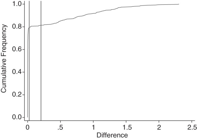
Cumulative frequency plot for the magnitude of the difference between the logit of the propensity score for a given exposed subject and the logit of the propensity score for the matched unexposed subject.

One way to select a caliper would be to use a statistic related to Youden's index (16) to determine the point that is closest to the upper left corner of the cumulative frequency plot in Figure 4. The cumulative frequency takes values from 0 to 1; if the magnitude of the difference in X between the exposed and unexposed subject in each matched pair were divided by the magnitude of the largest difference, then these scaled differences would also take values from 0 to 1. Youden's index could then be calculated as

and the value of the magnitude of the difference at which this index takes its maximum could be used as the caliper. This is how the position of the left-hand vertical line was selected.

The values selected by this method ranged from 0.002 to 0.06, tending to decrease as r increased and increase as β increased. In other words, a wider caliper was needed if there was a greater difference between exposed and unexposed subjects or if there were fewer unexposed subjects available to match, which seems intuitively sensible. On the other hand, the 0.25-standard deviation calipers ranged from 0.20 to 0.25 but tended to increase as r increased and decrease as β increased. The mean calipers selected by each method in each scenario are given in Web Table 1, available at http://aje.oxfordjournals.org/.

This method of selecting a caliper resulted in less bias when using all matching methods. The bias was reduced by approximately 50%–99% (85%–99% for the best-first method), whereas the number of matched pairs was reduced by only approximately 1%–10% (2%–4% for the best-first method). The mean numbers of pairs analyzed and mean reduction in bias for each scenario are given in Web Tables 2 and 3.

As shown in Table 4, there was no discernible remaining bias when using best-first matching, 5-to-1-digit matching, or matching in a random order, no matter the number of controls per case or the value of β. When using ascending and descending matching, the bias was reduced by at least a factor of 2, and the remaining bias represents less than 1% of the crude bias before matching in all scenarios, but it was still at least an order of magnitude greater than the bias when using the other methods.

Table 4.

Mean Difference in X Between Exposed and Unexposed Subjects When a Caliper Selected by Youden's Index^a is Applied, Using 5 Different Matching Methods

Matching Method by Controls per Case	OR for Effect of X on Exposure
	1.5	2	5	10
2
Ascendingb	−0.0060	−0.0107	−0.0138	−0.0124
Descendingc	0.0061	0.0119	0.0171	0.0164
Random orderd	0.0001	0.0004	0.0008	0.0014
Best firste	0.0001	0.0002	0.0003	0.0007
5-to-1-digitf	−0.0004	−0.0007	−0.0009	−0.0005
5
Ascending	−0.0005	−0.0012	−0.0066	−0.0078
Descending	0.0005	0.0012	0.0078	0.0096
Random order	0.0000	0.0000	0.0003	0.0005
Best first	0.0000	0.0000	0.0002	0.0002
5-to-1-digit	−0.0000	−0.0001	−0.0004	−0.0004
10
Ascending	−0.00012	−0.00026	−0.00326	−0.00536
Descending	0.00012	0.00026	0.00366	0.00640
Random order	0.00000	0.00000	0.00016	0.00032
Best first	0.00000	0.00001	0.00010	0.00014
5-to-1-digit	−0.00001	−0.00002	−0.00017	−0.00030
20
Ascending	−0.00003	−0.00006	−0.00150	−0.00343
Descending	0.00003	0.00006	0.00161	0.00397
Random order	0.00000	0.00000	0.00006	0.00019
Best first	0.00000	0.00000	0.00005	0.00009
5-to-1-digit	0.00000	0.00000	−0.00007	−0.00019

Abbreviation: OR, odds ratio.

^a For each point, Youden's index is the sum of the horizontal distance from the y-axis plus the vertical distance from the line y = 1.

^b In the ascending method, each time a match is made, the exposed subject with the lowest propensity score is used.

^c In the descending method, each time a match is made, the exposed subject with the highest propensity score is used.

^d In the random order method, each time a match is made, the exposed subject is selected at random.

^e In the best first method, each time a match is made, the exposed subject with the closest matching unexposed subject is used.

^f n the 5-to-1-digit method, initially, matched pairs are selected at random from exposed-unexposed pairs for which propensity score is identical to 5 decimal places (on a log-odds scale). When no such pairs remain, pairs are selected at random from those with identical scores to 4 decimal places, then to 3 decimal places, and so forth.

Closeness of matching

The closeness of matching, measured by the root mean squared difference, is shown in Table 5 for all scenarios with 5 controls per case.

Table 5.

Root Mean Squared Difference in X Between Exposed and Unexposed Subjects

Matching Method by Caliper	OR for Effect of X on Exposure
	2 Controls per Case				5 Controls per Case				10 Controls per Case				20 Controls per Case
	1.5	2	5	10	1.5	2	5	10	1.5	2	5	10	1.5	2	5	10
None
Ascendinga	0.2005	0.4653	0.9871	1.1479	0.0320	0.0985	0.5179	0.7145	0.0126	0.0345	0.3144	0.5124	0.0058	0.0155	0.1874	0.3696
Descendingb	0.0603	0.1583	0.5510	0.7395	0.0188	0.0399	0.2573	0.4237	0.0094	0.0196	0.1452	0.2877	0.0051	0.0112	0.0832	0.1976
Random orderc	0.1033	0.3016	0.7887	0.9661	0.0207	0.0563	0.3938	0.5823	0.0097	0.0226	0.2290	0.4080	0.0051	0.0118	0.1300	0.2879
Best firstd	0.1264	0.3750	0.9329	1.1149	0.0225	0.0665	0.4730	0.6814	0.0100	0.0246	0.2773	0.4818	0.0052	0.0124	0.1577	0.3417
5-to-1-digite	0.3871	0.7771	1.4478	1.6312	0.0908	0.2541	1.1178	1.4035	0.0487	0.0949	0.6857	1.1963	0.0230	0.0610	0.5942	0.9506
0.25 SD
Ascending	0.0368	0.0584	0.0790	0.0777	0.0110	0.0206	0.0534	0.0609	0.0059	0.0105	0.0389	0.0501	0.0033	0.0062	0.0269	0.0410
Descending	0.0389	0.0850	0.1368	0.1367	0.0112	0.0223	0.0976	0.1168	0.0059	0.0110	0.0668	0.0999	0.0033	0.0063	0.0408	0.0820
Random order	0.0247	0.0333	0.0452	0.0488	0.0097	0.0162	0.0349	0.0424	0.0054	0.0093	0.0283	0.0376	0.0032	0.0058	0.0217	0.0330
Best first	0.0200	0.0203	0.0178	0.0177	0.0090	0.0137	0.0160	0.0173	0.0053	0.0085	0.0152	0.0164	0.0032	0.0055	0.0140	0.0155
5-to-1-digit	0.0266	0.0265	0.0215	0.0203	0.0135	0.0168	0.0188	0.0180	0.0085	0.0116	0.0171	0.0169	0.0056	0.0080	0.0154	0.0155
Youden indexf
Ascending	0.0116	0.0195	0.0217	0.0199	0.0021	0.0038	0.0133	0.0138	0.0009	0.0014	0.0083	0.0109	0.0004	0.0006	0.0050	0.0082
Descending	0.0118	0.0207	0.0246	0.0225	0.0021	0.0039	0.0146	0.0156	0.0009	0.0014	0.0088	0.0121	0.0004	0.0006	0.0051	0.0088
Random order	0.0085	0.0119	0.0113	0.0109	0.0019	0.0034	0.0080	0.0077	0.0008	0.0014	0.0058	0.0065	0.0004	0.0006	0.0040	0.0053
Best first	0.0079	0.0099	0.0074	0.0069	0.0019	0.0032	0.0060	0.0052	0.0008	0.0013	0.0049	0.0047	0.0004	0.0006	0.0036	0.0041
5-to-1-digit	0.0095	0.0127	0.0093	0.0080	0.0026	0.0039	0.0069	0.0060	0.0011	0.0019	0.0052	0.0053	0.0005	0.0008	0.0037	0.0044

Abbreviations: OR, odds ratio; SD, standard deviation.

^a In the ascending method, each time a match is made, the exposed subject with the lowest propensity score is used.

^b In the descending method, each time a match is made, the exposed subject with the highest propensity score is used.

^c In the random order method, each time a match is made, the exposed subject is selected at random.

^d In the best first method, each time a match is made, the exposed subject with the closest matching unexposed subject is used.

^e In the 5-to-1-digit method, initially, matched pairs are selected at random from exposed-unexposed pairs for which propensity score is identical to 5 decimal places (on a log-odds scale). When no such pairs remain, pairs are selected at random from those with identical scores to 4 decimal places, then to 3 decimal places, and so forth.

^f For each point, Youden's index is the sum of the horizontal distance from the y-axis plus the vertical distance from the line y = 1.

In the absence of a caliper, the descending method provides the best matches, particularly when there is a large separation between exposed and unexposed subjects. However, if a caliper is used, the matches are much closer. The best-first method gives the closest matches, and the ascending method may perform better than the descending method, depending on the separation between exposed and unexposed subjects. With a tight caliper, there is little difference between the methods in terms of closeness of matches, although the best-first, random, and 5-to-1-digit methods are generally slightly better than the ascending and descending methods. Tightening the caliper from 0.25 standard deviations reduced the variance of the differences within matched pairs by between 75% and 98% (the mean reduction in variance in each scenario is given in Web Table 4).

DISCUSSION

These results show that the appropriate choice of caliper and the order in which matches are made can have a considerable effect on the quality of the matches achieved. In particular, matching without a caliper can lead to poor balance between treated and untreated subjects, even when there are plenty of untreated subjects from which to select matches. The best-first method of selecting matches produces the best matched sets in terms of minimizing bias, producing close matches, and minimizing the standard error of the difference between exposed and unexposed subjects.

The use of a caliper when matching can reduce the number of exposed subjects included in the analysis. Not only can this reduce the precision with which it is possible to estimate the effect of exposure (because of the reduced sample size), but it can also alter the estimand. It is no longer the effect of treatment in the treated subjects that is being estimated, but the effect of treatment in those treated subjects for whom we can find controls. This may differ from the effect in all of the treated subjects if the effect of the exposure varies with the covariates. For this reason, it would be very important to present the distribution of covariates in exposed subjects with and without matches, so that readers can judge whether results would apply to a particular population with a fixed distribution of covariates. Nonetheless, a tight caliper will result in an unbiased estimate of the effect of the exposure in a fixed population. Had a looser caliper that resulted in biased matches been used, the resulting estimate would have been a biased estimate for the effect of exposure in the treated subjects, and there would be no way of knowing whether there was a population in which that was the true effect, much less of identifying such a population.

This article has concerned itself only with nearest-neighbor pair matching, and other matching strategies might be better in cases where available controls are sparse. For example, matching with replacement allows the same control to be used as a match for a number of exposed subjects, which can increase the number of cases that can be included in the analysis. However, this will generally also reduce precision because there will be fewer matched sets to analyze (14) when several exposed subjects may be matched to the unexposed subject in a single matched set. This means that fewer unexposed subjects are included in the analysis, although they are closer matches to the exposed subjects than when matching without replacement. The order in which matches are made has no effect on the matching achieved when matching with replacement, so it was not considered in the comparisons here. However, the problems of selection when using a tight caliper also apply when matching with replacement, and if some exposed subjects cannot be matched, the population to which the estimated effect applies is changed, as discussed in the previous paragraph. Nonetheless, because nearest-neighbor pair matching is widely used, possibly because of the simplicity of the analysis and interpretation, having a reliable way to do this is important.

All of the methods compared here are greedy methods, in that once a match has been made, it is not reconsidered. There are optimal matching methods that will break matches if doing so can result in a better overall matched sample, and it has been shown that there are circumstances in which greedy matching will find fewer acceptable matches than optimal matching (17). However, optimal matching requires far greater computational resources, and the time required increases as a cubic function of the size of the data set, as opposed to a quadratic function for greedy matching. Hence, greedy methods may still be required for very large data sets.

This article presents only the effects of different matching methods on the balance of propensity score, not on the resulting bias in the estimate of the effect of exposure, which is ultimately what is of interest. However, the bias will depend on the strength of the association between covariates and outcome; large imbalances in covariates may not cause large biases if those covariates are only weakly associated with the outcome. However, if the covariates are well balanced, they cannot lead to large biases, and so a method that balances covariates well will always lead to an unbiased estimate.

The implementation of 5-to-1-digit matching used in this analysis differs in 2 respects from that implemented by Parsons (15). First, matching was based on the linear predictor of the propensity score rather the conditional probability of exposure. This was because that is how the other methods were implemented, and the definition of a caliper on the log-odds scale used by all of the other methods would be different on a probability scale.

Second, the range of potential matches was extended so that all cases could be matched when no caliper was applied, as happened with all of the other methods. So if no match was found to with 0.1 on the log-odds scale, matches to within 1 and then within 10 were attempted. Clearly, this will give far poorer matches than the standard implementation of this method, but it will be comparable to the other methods with no caliper, all of which would match all available cases.

The use of the Youden index (16) to determine the most appropriate caliper is viable only when best-first matching is used, because this is the only method for which the matches will not change when the caliper changes. Selecting in a random order and with 5-to-1-digit matching both have a random component to the selection of matches, which will obviously differ in different runs. With ascending and descending matching, a match that was made by using a wide caliper may not be made by using a narrower one and, hence, that control will be available for matching to a different case.

Mean times for matching with each method in each scenario are given in Web Table 5. Ascending and descending matches were the quickest methods in all scenarios considered, with 5-to-1-digit matching being an order of magnitude slower. Best-first matching took approximately 2–3 times as long as 5-to-1-digit matching, and longer if no caliper was applied. Matching in a random order was 2–10 times slower again, although no attempt was made to ensure the implementation was as efficient as possible. The Youden index is only 1 way to select an appropriate caliper. Given the number of simulations used here, an automated method was essential. In practice, the appropriate caliper may be wider (to give more matches, albeit poorer) or tighter. A cumulative frequency plot like that in Figure 4 can inform this decision.

Authors of previous studies examining the influence of caliper width have based the choice of caliper solely on mean squared error, which combines bias and precision in a single number (10, 11). However, the mean squared error of an unbiased estimator can be reduced by increasing the sample size, whereas the reduction in the mean squared error for a biased estimator will be much less for the same increase in sample size. Hence, the focus here on removing bias. Furthermore, although Raynor (10) considered how the strength of the association between the propensity score and outcome affected the choice of caliper, neither author considered how the appropriate caliper may depend on the difficulty of finding matches, as this article does.

The use of an appropriate caliper has been shown to be vital for achieving good matches. Matching cases in either ascending or descending order of the propensity score will generally provide poorer matches that the other matching methods and will make it difficult to select an appropriate caliper. Stata software (StataCorp LP, College Station, Texas) to implement best-first matching, matching in a random order, and 5-to-1-digit matching is available from the author's website (http://personalpages.manchester.ac.uk/staff/mark.lunt).

REFERENCES

- 1.Austin PC. A critical appraisal of propensity-score matching in the medical literature between 1996 and 2003. Stat Med. 2008;27(12):2037–2049. doi: 10.1002/sim.3150. [DOI] [PubMed] [Google Scholar]
- 2.Greenwood E. Experimental Sociology: A Study in Method. New York, NY: King's Crown Press; 1945. [Google Scholar]
- 3.Chapin F. Experimental Designs in Sociological Research. New York, NY: Harper; 1947. [Google Scholar]
- 4.Cochran WG, Rubin DB. Controlling bias in observational studies: a review. Sankhyā: Indian J Stat, Ser A. 1973;35(4):417–446. [Google Scholar]
- 5.Rubin DB. Matching to remove bias in observational studies. Biometrics. 1973;29(1):159–183. [Google Scholar]
- 6.Rubin DB. The use of matched sampling and regression adjustment to remove bias in observational studies. Biometrics. 1973;29(1):185–203. [Google Scholar]
- 7.Rosenbaum PR, Rubin DB. The central role of the propensity score in observational studies for causal effects. Biometrika. 1983;70(1):41–55. [Google Scholar]
- 8.Rubin DB, Thomas N. Matching using estimated propensity scores: relating theory to practice. Biometrics. 1996;52(1):249–264. [PubMed] [Google Scholar]
- 9.Rosenbaum PR, Rubin DB. Constructing a control group using multivariate matched sampling methods that incorporate the propensity score. Am Stat. 1985;39(1):33–38. [Google Scholar]
- 10.Raynor WJ., Jr Caliper pair-matching on a continuous variable in case-control studies. Commun Stat Theory Methods. 1983;12(13):1499–1509. [Google Scholar]
- 11.Austin PC. Optimal caliper widths for propensity-score matching when estimating differences in means and differences in proportions in observational studies. Pharm Stat. 2011;10(2):150–161. doi: 10.1002/pst.433. [DOI] [PMC free article] [PubMed] [Google Scholar]
- 12.Stuart EA. Matching methods for causal inference: a review and a look forward. Stat Sci. 2010;25(1):1–21. doi: 10.1214/09-STS313. [DOI] [PMC free article] [PubMed] [Google Scholar]
- 13.Caliendo M, Kopeinig S. Some practical guidance for the implementation of propensity score matching. J Econ Surv. 2008;22(1):31–72. [Google Scholar]
- 14.Dehejia RH, Wahba S. Propensity score matching methods for non-experimental causal studies. Rev Econ Stat. 2002;84(1):151–161. [Google Scholar]
- 15.Parsons LS. Reducing bias in a propensity score matched-pair sample using greedy matching techniques. Paper 214-26 in Proceedings of the Twenty-Sixth Annual SAS Users Group International Conference; Cary, NC: SAS Institute, Inc; 2001. [Google Scholar]
- 16.Youden WJ. Index for rating diagnostic tests. Cancer. 1950;3(1):32–35. doi: 10.1002/1097-0142(1950)3:1<32::aid-cncr2820030106>3.0.co;2-3. [DOI] [PubMed] [Google Scholar]
- 17.Rosenbaum PR. Optimal matching for observational studies. J Am Stat Assoc. 1989;84(408):1024–1302. [Google Scholar]
Associated Data
This section collects any data citations, data availability statements, or supplementary materials included in this article.