A role for the developing lexicon in phonetic category acquisition

Abstract

Infants segment words from fluent speech during the same period when they are learning phonetic categories, yet accounts of phonetic category acquisition typically ignore information about the words in which sounds appear. We use a Bayesian model to illustrate how feedback from segmented words might constrain phonetic category learning by providing information about which sounds occur together in words. Simulations demonstrate that word-level information can successfully disambiguate overlapping English vowel categories. Learning patterns in the model are shown to parallel human behavior from artificial language learning tasks. These findings point to a central role for the developing lexicon in phonetic category acquisition and provide a framework for incorporating top-down constraints into models of category learning.

One of the first challenges for language learners is deciding which speech sound distinctions are and are not relevant in their native language. Learning to group perceptual stimuli into categories is a complex task. Categories often overlap, and boundaries are not always clearly defined. This is especially apparent when one looks at sound categories that occur in natural language. Phonetic categories, particularly vowel categories, show substantial acoustic overlap (Figure 2a).¹ Even a single speaker’s productions of a specific category in a specific context are variable. Phonetic categories contain even more variability across ranges of speakers and contexts. The high degree of overlap suggests that infants learning language sometimes need to attend carefully to slight differences in pronunciation between different categories while simultaneously ignoring large degrees of within-category variability.

Figure 2.

Results from Simulation 1. Ellipses delimit the area corresponding to 90% of vowel tokens corresponding to (a) vowel categories for all speakers from Hillenbrand et al. (1995) that were used to generate the first corpus and the resulting categories found by (b) the gradient descent algorithm and (c) the infinite mixture model; and (d) vowel categories for men only from Hillenbrand et al. (1995) that were used to generate the second corpus and the resulting categories found by (e) the gradient descent algorithm and (f) the infinite mixture model.

Infants nevertheless appear to learn about the sound categories of their native language quite early. Babies initially discriminate sound contrasts whether or not they are functionally useful in the native language, but this ability declines for most non-native consonant contrasts between six and twelve months of age (Werker & Tees, 1984). During the same period, infants’ ability to discriminate perceptually difficult consonant contrasts in their native language is enhanced (Narayan, Werker, & Beddor, 2010). Vowel perception begins to reflect the learner’s native language as early as six months (Kuhl, Williams, Lacerda, Stevens, & Lindblom, 1992). These perceptual changes are generally interpreted as evidence for infants’ developing knowledge of native phonetic categories, implying that young learners have a remarkable ability to acquire speech sound categories amidst high acoustic overlap.

Identifying the mechanisms that support infants’ early language learning abilities has been a central focus of research in language acquisition. Statistical learning theories propose that infants acquire each layer of structure by observing statistical dependencies in their input. Infants show robust sensitivity to statistical patterns. They extract phonological and phonotactic regularities that govern sound sequences (Seidl, Cristiá, Bernard, & Onishi, 2009; White, Peperkamp, Kirk, & Morgan, 2008), use transitional probabilities to segment fluent speech into word-sized units (Pelucchi, Hay, & Saffran, 2009; Saffran, Aslin, & Newport, 1996), and notice adjacent and non-adjacent dependencies between words in grammar learning tasks (Gómez, 2002; Gómez & Gerken, 1999). Learners are also sensitive to statistical structure in non-linguistic stimuli such as visual shapes (Fiser & Aslin, 2002) and auditory tones (Saffran, Johnson, Aslin, & Newport, 1999), suggesting that statistical learning is a domain general strategy for discovering structure in the world.

Distributional learning has been proposed as a statistical learning mechanism for phonetic category acquisition (Maye & Gerken, 2000; Maye, Werker, & Gerken, 2002). Learners are hypothesized to obtain information about which sounds are contrastive in their native language from the distributions of sounds they hear. Learners hearing a bimodal distribution of sounds along a particular acoustic dimension can infer that the language contains two categories along that dimension; conversely, a unimodal distribution provides evidence for a single phonetic category. Distributional learning is consistent with empirical evidence showing that infants attend to distributional cues at the age when they are first learning phonetic categories (Maye et al., 2002). Computational modeling results also suggest that a distributional learning strategy can be successful at recovering phonetic categories that have sufficient separation in acoustic space (McMurray, Aslin, & Toscano, 2009; Vallabha, McClelland, Pons, Werker, & Amano, 2007). However, distributional learning is less effective when categories have a high degree of overlap. Overlapping categories pose a problem because the distribution of sounds in two overlapping categories can appear unimodal (Figure 1), misleading a learner into believing there are too few categories.

Figure 1.

The problem of overlapping categories. (a) Distribution of sounds in two overlapping categories. The points were sampled from the Gaussian distributions representing the /ɪ/ and /e/ categories based on men’s productions. (b) These sounds appear as a unimodal distribution when unlabeled, creating a difficult problem for a distributional learner.

In this article, we show that learners can overcome the problem of overlapping categories by using feedback from higher levels of structure to constrain category acquisition. Specifically, we show that using feedback from a developing lexicon can improve phonetic category acquisition. Interactive learning of words and sounds is beneficial when sounds occur in distinct lexical contexts. The blue and red categories from Figure 1 overlap acoustically when considered in isolation, but an interactive learner can notice that, for example, the blue sounds occur in the word milk and the red sounds occur in the word game. These lexical contexts are easily distinguishable on the basis of acoustic information and can be used as disambiguating cues to sound category membership. This type of interactive learning does not require meanings or referents to be available to the learner; it requires only that learners use acoustic information to categorize word tokens. Thus, information from lexical contexts has the potential to contribute to early development, even before infants have learned the meanings of many words. Our theoretical framework is similar to that proposed by Swingley (2009), but here we provide a formal account of this interactive learning hypothesis. Our analysis is framed at Marr’s (1982) computational level, examining the statistical solution to the sound category learning problem in a structured environment where sounds are organized into words. We quantitatively investigate the potential benefit of interactive learning by building a computational model that learns to categorize sounds and words simultaneously and show that word-level information provides an informative cue that can help learners acquire phonetic categories.

Although our focus in this article is on linguistic categories, the modeling that we develop here may well have broader application. Distributional learning, for example, can be thought of as a domain general strategy for recovering underlying structure. Learning mechanisms that rely on probability density estimation, in which categories are defined by their probability of producing different stimuli, are popular in research on categorization (Ashby & Alfonso-Reese, 1995). The specific models that have been proposed as accounts of phonetic category learning (e.g., Gaussian mixture models, de Boer & Kuhl, 2003; Vallabha et al., 2007; McMurray et al., 2009; Toscano & McMurray, 2010; Dillon, Dunbar, & Idsardi, 2013) have also been proposed as accounts of category learning more generally (Anderson, 1990; Rosseel, 2002; Sanborn, Griffiths, & Navarro, 2010). While studies of category learning have tended to focus on the acquisition of categories in isolation from their context, earlier work on the effects of prior knowledge on category learning (e.g., Pazzani, 1991; Heit & Bott, 2000; Wattenmaker, Dewey, Murphy, & Medin, 1986; Murphy & Allopenna, 1994) and more recent work on the consequences of learning multiple categories simultaneously (Gureckis & Goldstone, 2008; Canini, Shashkov, & Griffiths, 2010; Canini & Griffiths, 2011) suggests that our conclusions about the importance of using information from multiple levels of structure may have implications beyond just language acquisition.

In the following, we first introduce the idea of modeling category learning as density estimation and show how distributional learning can be viewed in this framework. We then show through an initial simulation that distributional learning can be challenging when categories have a high degree of overlap. Our next section explores how constraints from higher-level structure might supplement distributional learning, formalizing a lexical-distributional model that learns word- and sound-level information simultaneously. Three simulations quantify the benefit of interactive learning by comparing performance of our lexical-distributional model directly to that of distributional models. We conclude by showing that qualitative behavior of our lexical-distributional model mirrors patterns from experiments on sound category learning, suggesting that people behave as interactive learners, and by discussing the plausibility of the interactive learning approach for language acquisition and for category learning more generally.

Distributional learning

Rational analyses of category learning (e.g., Anderson, 1990; Ashby & Alfonso-Reese, 1995) reduce the psychological problem of learning a new category to the statistical problem of density estimation: Learning a category requires estimating a probability distribution over the items that belong to the category. A learner can use the resulting distributions to quickly decide which category a new item belongs to, with categorization being a simple matter of probabilistic inference. This perspective provides a novel interpretation of traditional models of categorization such as prototype and exemplar models (Ashby & Alfonso-Reese, 1995) and provides a productive link between ideas from statistics and theories of human category learning (Griffiths, Sanborn, Canini, Navarro, & Tenenbaum, 2011).

Distributional learning accounts of early language acquisition (Maye et al., 2002) likewise propose that phonetic category acquisition can be viewed as a density estimation problem. That is, adult-like discrimination and processing abilities are assumed to reflect knowledge of the distributions associated with native language phonetic categories. Distributional learning specifies one way in which this knowledge might be acquired: Learners observe sounds in their input that cluster in perceptual space and hypothesize categories to coincide with the locations of those clusters. They can use the clusters they observe to estimate the probability distribution associated with each category. This gives them a way of simultaneously learning which categories are in their language and which sounds are associated with each category.

Distributional learning is supported by experimental evidence that infants are sensitive to distributions of sounds at six and eight months. Maye et al. (2002) familiarized infants with stop consonants ranging from unaspirated [t] to [d]. Although these sounds occur as variants of different phonemes in English, they are not used contrastively, and always appear in different phonological environments. Adults have previously been shown to have difficulty distinguishing these sounds in laboratory settings, whereas young infants are sensitive to the distinction (Pegg & Werker, 1997). Maye et al. investigated infants’ ability to use statistical information to constrain how they interpret these sounds. During familiarization, infants heard either a bimodal distribution of sounds, mimicking the distribution that might be associated with two phonetic categories, or a unimodal distribution, mimicking the distribution that might be associated with a single phonetic category. Infants who heard the sounds embedded in a bimodal distribution exhibited better discrimination of the endpoint stimuli at test than infants who heard the sounds embedded in a unimodal distribution, suggesting that participants’ sensitivity to this contrast had changed to reflect the distributions of sounds that they heard. Bimodal distributions can also facilitate discrimination of a difficult voicing continuum (Maye, Weiss, & Aslin, 2008) and of a place of articulation continuum (Yoshida, Pons, Maye, & Werker, 2010) in infants. Adults retain sensitivity to distributional information in consonants (Maye & Gerken, 2000) and vowels (Gulian, Escudero, & Boersma, 2007), though sensitivity to distributional cues appears to decrease as phonetic category acquisition progresses (Yoshida et al., 2010).

The period around six to eight months when infants show sensitivity to distributional information corresponds closely to the period of time when infants lose sensitivity to non-native contrasts (Werker & Tees, 1984). This suggests that learners can make use of distributional information during the time when they are acquiring phonetic categories, and it is intuitively plausible that finding clusters of sounds would be a useful strategy for acquiring phonetic categories. Computational modeling allows us to look more carefully at the predicted outcome of distributional learning to determine whether infants’ sensitivity would be predicted to facilitate phonetic category acquisition. If computational models can recover the sound categories of a natural language through a purely distributional learning strategy, then this would lend credence to the possibility that infants can do the same. The remainder of this section provides an overview of computational models that have been used to investigate the utility of distributional learning for phonetic category acquisition.

Mixture models

Models of phonetic category acquisition have implemented distributional learning by assuming that learners need to find the set of categories that describe the distribution of sounds in acoustic space, where each category is represented by a Gaussian (i.e., normal) distribution (de Boer & Kuhl, 2003; Dillon et al., 2013; McMurray et al., 2009; Toscano & McMurray, 2010; Vallabha et al., 2007). In this framework, phonetic category learning consists of jointly inferring the mean, covariance, and frequency of each Gaussian category as well as the category label of each sound. This inference process has been implemented through a type of model known as a Gaussian mixture model, which has also appeared in the general literature on category learning (Anderson, 1990; Rosseel, 2002; Sanborn et al., 2010). By comparing the outcome of learning in these models to the true set of phonetic categories in a language, we can gain insight into the plausibility of distributional learning as a mechanism for phonetic category acquisition.

Mixture models assume that there are several categories and that each of the observed data points was generated from one of these categories. In phonetic category acquisition, the categories are phonetic categories and the data points represent speech sounds. Mixture models typically assume that there is a fixed number of categories C; here we refer to each category by a number c ranging from 1 to C. Each category is associated with a probability distribution p(x|c) which defines the probability of generating a stimulus value x from category c. The probability distribution p(x|c) in mixture models can take a variety of forms, but here we focus on the case in which p(x|c) is a Gaussian distribution, so that recovering p(x|c) is equivalent to recovering a mean μ_c and a covariance matrix Σ_c. The observed data points are referred to as x_i. Each data point is assumed to be associated with a label z_i, ranging between 1 and C, that indicates which category it belongs to. In an unsupervised learning setting such as language acquisition, the labels z_i are unobserved. Learners need to recover the probability distribution p(x|c) associated with each category as well as the label z_i associated with each data point.

Inferring a probability distribution p(x|c) is straightforward when a learner knows which stimuli belong to the category (i.e., when z_i is known). If p(x|c) is a Gaussian distribution, the parameter estimates for μ and Σ that maximize the probability of the data are given by the empirical mean and covariance

$$\begin{array}{l}{\mu }_c=\frac{1}{n}\sum _{z_i=c}{x}_i\\ {\mathrm{\sum }}_c=\frac{1}{n}\sum _{z_i=c}(x_i-\mu ){(x_i-\mu )}^T\end{array}$$ (1)

where n denotes the number of observed data points x_i for which z_i = c. These equations give optimal estimates for category parameters when a learner has no prior knowledge about what the category mean and covariance should be, but it is also straightforward to incorporate prior beliefs about these parameters in a Bayesian framework using a type of prior distribution known as a normal inverse Wishart distribution (see Gelman, Carlin, Stern, & Rubin, 1995, for details).

Conversely, if the probability density function p(x|c) and frequency p(c) associated with each category is known, it is straightforward to infer z_i, assigning a novel unlabeled data point to a category. This amounts to using Bayes’ rule,

$$p(c\mid x)=\frac{p(x\mid c)p(c)}{{\displaystyle \sum _{c^{\prime }=1}^C}p(x\mid c^{\prime })p(c^{\prime })}$$ (2)

to compute the posterior probability of category membership, where x is the unlabeled stimulus, c denotes a particular category, and the sum in the denominator ranges over the set of all possible categories.

The problem faced by language learners acquiring phonetic categories is difficult because neither category assignments z_i for individual stimuli, nor probability density functions p(x|c) associated with phonetic categories, are known in advance. This produces a type of chicken-and-egg learning problem that is common to many problems in language acquisition. Algorithms such as Expectation Maximization (EM) (Dempster, Laird, & Rubin, 1977) provide a principled solution to these types of problems by searching for the parameters and category labels that maximize the probability of the data. In phonetic category acquisition, learners using the EM algorithm would begin with an initial hypothesis about the category density functions, then iterate back and forth between inferring category assignments for each sound they have heard according to Equation 2 and inferring probability density functions for each category according to Equation 1.

The EM algorithm has been used to test distributional models on English vowel categories. de Boer and Kuhl (2003) fit Gaussian mixture models to actual formant values in mothers’ spontaneous productions of the /a/, /i/, and /u/ phonemes from the words sock, sheep, and shoe. They compared model performance from infant- and adult-directed speech and found better performance when the models were trained on infant-directed speech, as measured by the accuracy of the inferred category centers. This benefit of infant-directed speech as training data was attributed to the increased separation between categories that is typical of infant-directed speech (Kuhl et al., 1997; but see McMurray, Kovack-Lesh, Goodwin, & McEchron, submitted). However, note that the /i/, /u/, and /a/ vowel categories used by de Boer and Kuhl (2003) are precisely those vowel categories with maximal separation in acoustic space, and children acquiring a full set of phonetic categories would face a more difficult problem. We return to the issue of category separation below.

Inferring the number of categories

The EM algorithm requires the number of categories to be specified in advance. However, it is unlikely that human learners know in advance how many phonetic categories they will be learning, because this number varies across languages. McMurray et al. (2009) and Vallabha et al. (2007) proposed an online sequential learning algorithm similar to EM that provides a way around this limitation. The algorithm resembles EM in that it iterates between estimation of category parameters and assignment of a sound to a particular category. During each iteration the model observes a single speech sound and assigns it to a category. It then updates the mean, covariance, and frequency parameters of each category on the basis of that sound (see Vallabha et al., 2007, for a detailed description of these updates, which proceed by a method of gradient descent). Automatic inference of the number of categories is achieved by eliminating categories whose frequency drops below a predefined threshold. The model begins with a high number of phonetic categories and prunes those that are not needed.

Nonparametric Bayesian models provide a second option for flexibly learning the number of categories. A type of nonparametric Bayesian model known as the Dirichlet process (Ferguson, 1973) has been used to model category learning in language and other domains (Anderson, 1990; Goldwater, Griffiths, & Johnson, 2009, 2011; M. Johnson, Griffiths, & Goldwater, 2007; Sanborn et al., 2010). Dirichlet processes provide a modeling framework similar to the mixture models described above, but they differ from traditional mixture models in that they provide a mechanism for inferring an unbounded number of categories. Because of this, Dirichlet process models are often referred to as infinite mixture models (IMM). They infer the correct number of categories by considering a potentially infinite number of categories but encoding a prior bias toward fewer categories. This bias in the prior distribution encourages the model to use only those categories that are necessary to explain the data. Here we implement distributional learning using the infinite Gaussian mixture model (Rasmussen, 2000), which assumes that the probability density function p(x|c) associated with each category is Gaussian. We use Gibbs sampling (Geman & Geman, 1984), a form of Markov chain Monte Carlo, as an inference algorithm for this model. The details of the model and inference algorithm are given in Appendix A.

The gradient descent models and the IMM each provide a way of inferring the number of categories present in the data, and each can be evaluated on its ability to recover the correct number of categories. Previous work has examined this ability in both types of models. Using the gradient descent method, McMurray et al. (2009) focused on a voicing contrast in consonants. They generated training data for the models by sampling sounds from Gaussian distributions that mimicked the voice onset time (VOT) distributions of voiced and voiceless stops, then showed that their learning algorithm recovered these two categories correctly. Vallabha et al. (2007) performed similar experiments using vowels. They generated training data that mimicked the distributions associated with single speakers producing /i/, /ɪ/, /e/, and /ε/ in English or /i/, /iː/, /e/, and /eː/ in Japanese. The most frequent learning outcome for models trained on these data was to recover four categories in each case. Models trained on English input data recovered categories that were distinguished along all three relevant dimensions (F₁, F₂, and duration), whereas models trained on Japanese input data recovered categories that were distinguished primarily by F₁ and duration. For both consonants and vowels, then, the gradient descent algorithm has yielded initial success in inferring the correct number of categories.

Dillon et al. (2013) examined the performance of the IMM in acquiring a three-category vowel system from Inuktitut. They considered the possibility that the model might acquire categories at either the phonemic level (3 categories) or the phonetic level (6 categories). Simulations showed that given different sets of parameters, the model could acquire either three or six categories, supporting a successful outcome of distributional learning. However, the authors also identified several ways in which the models’ solutions were insufficiently accurate to provide input for learning higher levels of linguistic structure.

Despite the success of these models, it is not yet clear whether distributional learning can accommodate more realistic input data. Phonetic categories, particularly vowel categories, can show a high degree of overlap (e.g. Peterson & Barney, 1952; Hillenbrand, Getty, Clark, & Wheeler, 1995), whereas the input data to these computational models contained only limited category overlap. Categories involved in the voicing contrast from McMurray et al. (2009) are well separated. The vowel contrasts used by Vallabha et al. (2007) were composed of neighboring categories that presumably had some degree of overlap, but even here, each model was trained on data from a single speaker. The training data therefore had lower within-category variability than one would expect to find in real language input, and this presumably led to a lower degree of overlap. The data used by Dillon et al. (2013) contained higher amounts of category overlap, but in this case the authors identified several shortcomings in the distributional model’s performance. Because their paper used the IMM, and used training data that did not conform to their Gaussian assumptions, it is difficult to compare their results directly to those obtained through the gradient descent algorithm on data generated from Gaussians. Our initial simulation tests both types of distributional learning models directly on a single dataset in which the categories have a high degree of overlap, comparing this to performance on a dataset in which categories have a lower degree of overlap.

Simulation 1: The problem of overlapping categories

Overlap between categories can potentially make the learning problem more difficult because the distribution of sounds from two categories can appear unimodal, misleading a distributional learner into assigning the sounds to one category. To explore this challenge, we test the ability of distributional learning models to recover the vowel categories from Hillenbrand et al. (1995). These categories exhibit high acoustic variability and therefore provide a challenging test case for distributional models.

Our simulations use two distributional learning models: the gradient descent algorithm from Vallabha et al. (2007) and the IMM. Each model provides a unique set of advantages. The gradient descent model has been used previously to investigate phonetic category acquisition, and its use here facilitates comparison with this previous work. Its algorithm is sequential and is thus arguably more psychologically plausible than the Gibbs sampling algorithm used with the IMM (but see Sanborn et al., 2010, for a sequential algorithm that can be used with the IMM). However, the drawback of using gradient descent is that the model cannot find a set of globally optimal category parameters, and instead converges to a locally optimal solution. The Gibbs sampling algorithm used with the IMM has some potential to overcome the problem of local optima. Furthermore, there is a straightforward way to extend the IMM to incorporate multiple layers of structure (Teh, Jordan, Beal, & Blei, 2006), and we take advantage of this flexibility to create the interactive lexical-distributional learning model introduced in the next section. Using the IMM as a distributional learning model thus allows for a direct comparison between the distributional and lexical-distributional learning strategies.

Throughout this article, we evaluate models on their ability to recover the correct number of categories, a measure that has become standard for evaluating success in unsupervised models of phonetic category learning (e.g. Dillon et al., 2013; McMurray et al., 2009; Vallabha et al., 2007). In addition, to assess the quality of these categories, we evaluate the models’ ability to identify which sounds from the corpus are in each category. Our analyses look at the categories recovered by each model, rather than at the models’ ability to use those categories in specific psycholinguistic tasks. Our assumption is that a learning strategy that supports robust category learning would also support use of those categories, either implicitly or explicitly, in psycholinguistic tasks.

Methods

Corpus preparation

Phoneme and word frequencies were obtained from the CHILDES parental frequency count (MacWhinney, 2000; Li & Shirai, 2000). We converted all words in the frequency data to their corresponding phonemic representations using the CMU pronouncing dictionary. If the dictionary contained multiple phonemic forms for a word, the first was used. Stress markings were removed, diphthongs /aʊ/, /aɪ/, and /ɔɪ/ were converted to sequences of two phonemes, and /ɝ/ was treated as a single phoneme rather than a sequence of two phonemes. Any words whose orthographic representation in CHILDES contained symbols other than letters of the alphabet, hyphen, and apostrophe were excluded. In addition, words not found in the CMU pronouncing dictionary were excluded. This resulted in the exclusion of 7,911 types, representing 28,447 tokens (approximately 1% of tokens), and left us with a phonematized word list of 15,825 orthographic word types, representing 2,548,494 tokens. This phonematized word list was used to compute empirical probabilities for each vowel (Table 1) for constructing the corpora in Simulations 1 and 2 and to directly sample word tokens for constructing the corpora in Simulations 3 and 4.

Table 1.

Normalized empirical probabilities of each vowel computed from the phonematized CHILDES parental frequency count.

Vowel	Empirical probability in word tokens	Empirical probability in word types
/æ/	0.080	0.068
/ɑ/	0.125	0.105
/ɔ/	0.038	0.035
/ε/	0.067	0.075
/e/	0.039	0.048
/ɝ/	0.035	0.083
/ɪ/	0.177	0.169
/i/	0.077	0.099
/o/	0.061	0.041
/ʊ/	0.041	0.019
/ʌ/	0.176	0.229
/u/	0.083	0.030

We obtained phonetic category parameters from production data collected by Hillenbrand et al. (1995). Production data by men, women, and children were used to compute empirical estimates of category means and covariances in the two-dimensional space given by the first two formant values using Equation 1. This gave us a set of phonetic categories with high variability and therefore high overlap among neighboring categories. To obtain parameters for a set of categories with lower overlap, we estimated means and covariances based only on productions by men. Note that schwa was absent both from the production data from Hillenbrand et al. (1995) and from the CMU pronouncing dictionary. Thus, schwa was not included as a vowel in any of our simulations.

Vowel tokens in each corpus were sampled from these Gaussian distributions. The same Gaussian parameters were used to sample each token of a phonetic category that appeared in a corpus; the acoustic values in the corpora thus did not reflect any contextual (e.g., coarticulatory) effects, and conformed to the Gaussian assumptions of all the models tested.

For Simulation 1, token frequencies from Table 1 were used to sample the labels z_i for two corpora of 20,000 vowels each. To produce each acoustic value x_i, a set of formant values was sampled from the Gaussian distribution associated with category z_i. The first corpus used phonetic category distributions computed from all speakers’ productions, and the second corpus used phonetic category distributions computed from men’s productions only. This created two corpora consisting of 20,000 F₁-F₂ pairs, one with high within-category variability and one with lower within-category variability. The label for each sound z_i was not provided to the models as training data, but was used for model evaluation.

Simulation parameters

Parameters used for the gradient descent algorithm were based on those from Vallabha et al. (2007). Like McMurray et al. (2009), however, we found that the initial category variance parameter C_r affected performance of this algorithm. Here we present results using C_r = 0.02, which we found to yield quantitatively and qualitatively better results than the value of 0.2 used by Vallabha et al. (2007). Other parameters, including the number of sweeps and the learning rate parameter, were identical to those used by Vallabha et al. Note that although we used 50,000 sweeps, the training data consisted of only 20,000 points; thus, training points were reused over the course of learning.

Parameters in the IMM include the strength of bias toward fewer phonetic categories and the model’s prior beliefs about phonetic category means and covariances. The bias toward fewer phonetic categories is controlled by the concentration parameter α_C, with smaller values corresponding to stronger biases. We explored a range of values for this parameter and found little effect on model performance; these simulations use a value of α_C = 10. The prior distribution over phonetic category parameters G_C is a normal inverse Wishart distribution that is controlled by three parameters: m₀, S₀, and ν₀. These parameters can be thought of as reflecting the mean, sum of squared deviations from the mean, and number of data points in a small amount of pseudodata that the learner imagines having assigned to each new category. Parameters were set to $m_0=\left[\begin{array}{c}500\\ 1500\end{array}\right],S_0=\left[\begin{array}{cc}1& 0\\ 0& 1\end{array}\right]$, and ν₀ = 1.001. They therefore encoded a bias toward the center of vowel space that was made as weak as possible² so that it could be overshadowed by real data.

Evaluation

Model performance was evaluated quantitatively by measuring the number of categories recovered by each model and computing two pairwise measures of performance, the F-score and variation of information (VI), which are described in detail in Appendix C. The F-score is a pairwise performance measure that is the harmonic mean of pairwise precision and recall, which are often referred to as accuracy and completeness in the psychology literature. It measures the extent to which pairs of points are correctly categorized together, and ranges between zero and one, with higher numbers corresponding to better performance. VI is a symmetric measure that evaluates the information theoretic difference between the true clustering and the clustering found by the model. It is a positive number, with lower numbers corresponding to better performance. Both performance measures require category assignments for each sound in the corpus. For the IMM we used the category assignments from the final iteration of the Gibbs sampling algorithm; these should correspond to a sample from the posterior distribution on category assignments. The gradient descent learning algorithm does not directly yield a set of category assignments, but we obtained assignments by sampling from the posterior distribution over categories, p(c|x) (Equation 2), for each sound.

Results and discussion

Results from each model are shown in Table 2 and illustrated in Figure 2. Whereas twelve categories were used to generate the corpus, the gradient descent model from Vallabha et al. (2007) recovered only six categories from the corpus with high category overlap and eight categories from the corpus with lower category overlap. The IMM recovered ten and eleven categories from these two corpora, respectively. However, the higher number of categories found by the IMM did not lead to better performance on the quantitative measures in either case. This is likely due to the fact that the extra category divisions found by the IMM did not match precisely with the true category divisions. For example, the long diagonal category in Figure 2c does not correspond to a true category, and even in Figure 2f, the division between the /ɪ/ and /e/ categories is incorrect. Neither model was able to recover the twelve categories used to generate the data. This was true of both corpora, but the problem was more pronounced in the corpus with high acoustic overlap between categories.

Table 2.

Phonetic categorization scores from the infinite mixture model (IMM) and gradient descent algorithm (GD) in Simulation 1.

	All Speakers		Men Only
	IMM	GD	IMM	GD
Number of categories	10	6	11	8
F-score	0.453	0.480	0.699	0.727
Variation of information	3.195	2.677	1.678	1.440

Note: The true number of phonetic categories is 12.

These results highlight the potential problem posed by overlapping categories. Often, tests of distributional learning are conducted on corpora in which vowels have an artificially low degree of overlap. de Boer and Kuhl (2003) selected three vowels with a large degree of separation, and Vallabha et al. (2007) removed speaker variability from the training data. Our simulations suggest that this lower degree of overlap between categories may have been critical to the models’ success. This corroborates the findings of Dillon et al. (2013) and suggests that more realistic data can potentially pose a problem for the types of distributional learning models that simply look for clusters of sounds in the acoustic input.

Our results from this simulation should be interpreted with caution, as it is not clear to what extent we have over- or underestimated the difficulty of the learning problem. Some degree of overlap can be overcome by using additional dimensions such as duration (Vallabha et al., 2007) and formant trajectories (Hillenbrand et al., 1995), and augmenting the data with information from these extra dimensions has the potential to improve performance in both models. Learning might also be supported by the increased separation between category means found in infant-directed speech (Kuhl et al., 1997), though it is not yet clear whether this advantage persists when one considers the increased within-category variability of infant-directed speech, especially for contrasts that do not involve the point vowels /a/, /i/, and /u/ (Cristia & Seidl, in press; McMurray et al., submitted). Cristia and Seidl, for example, suggest that some vowel contrasts may be hypoarticulated, that is, less distinct in infant-directed speech than in adult-directed speech. However, it is possible the data used in this simulation were simply too impoverished to support acquisition of a full vowel system in either models or humans. Because our training data were sampled from Gaussian distributions, the IMM is also likely to show better performance if trained on a larger corpus, though this would not necessarily be the case for non-Gaussian data. On the other hand, additional variability beyond what is reflected in Figure 2a is likely to arise through contextual variation, such as coarticulation with neighboring sounds, making the learning problem more difficult than is evident from the Hillenbrand et al. data. On the basis of our results, we wish to merely suggest the possibility that distributional learning may not be as robust as is often assumed. It is therefore important to consider possible supplementary learning mechanisms that could lead to more robust acquisition of phonetic categories. We propose one alternative strategy that children might use for learning phonetic categories, following Swingley (2009): if children are able to learn information about words and sounds simultaneously, they can use word-level information to supplement distributional learning.

Incorporating lexical constraints

Young infants show evidence of segmenting word-sized units at the same time that they are acquiring phonetic categories. Eight-month-olds track transitional probabilities of the speech they hear, discriminating words from non-words and part-words based purely on this statistical information (Saffran et al., 1996). Older infants can learn to map these segmented words onto referents (Graf Estes, Evans, Alibali, & Saffran, 2007), suggesting that infants use their sensitivity to transitional probabilities to begin learning potential wordforms for their developing lexicon. Studies using more naturalistic stimuli have demonstrated that infants can use stress and other cues to segment words from sentences and map these segmented words onto words they hear in isolation. Six-month-old infants can use familiar words such as Mommy to segment neighboring monosyllablic words from fluent sentences (Bortfeld, Morgan, Golinkoff, & Rathbun, 2005), and a more general ability to segment monosyllabic and bisyllabic words develops over the next several months (Jusczyk & Aslin, 1995; Jusczyk, Houston, & Newsome, 1999), during the same time that discrimination of non-native sound contrasts declines.

Segmentation tasks with naturalistic stimuli require infants not only to attend to segmentation cues, but also to ignore the within-category variability that distinguishes different word tokens. Infants need to recognize that the words heard in isolation are instances of the same words that they heard in fluent speech. There can be substantial acoustic differences among these different word tokens. Thus, infants as young as six months, who presumably have not yet finished acquiring native language phonetic categories, appear to be performing some sort of rudimentary categorization of the words they segment from fluent speech. Although young infants may not know meanings of these segmented words, they seem to be categorizing the word tokens on the basis of acoustic properties. This suggests a learning trajectory in which infants simultaneously learn to categorize both speech sounds and words, potentially allowing the two learning processes to interact.

Interaction between sound and word learning is not present in distributional learning theories. Distributional learning treats each sound in the corpus as being independent of its neighbors, ignoring higher level structure. The independence assumption has been present in both empirical and computational work. In experiments, infants have heard only isolated syllables during familiarization. This type of familiarization forces infants to treat those syllables as isolated units. Models of distributional learning similarly assume that infants consider only isolated sounds. In fact, distributional learning is precisely the type of statistical solution to the category learning problem that a learner should use if sounds were generated independently of their neighbors.

Here we demonstrate the importance of higher level structure by considering the optimal solution to the phonetic category learning problem when one assumes that sounds are instead organized into words. Throughout the remainder of this article, we will distinguish between words, acoustic tokens in the corpus, and lexical items, categories (word types) that represent groupings of acoustic tokens. Just like speech sounds are categorized into phonetic categories, we will assume that words are categorized into lexical items. Given this distinction, we can now use our Bayesian framework to define a lexical-distributional model that acquires phonetic categories and lexical items. Our model differs from distributional models in the hypothesis space it assigns to learners. A distributional model’s hypotheses consist of sets of phonetic categories, and learners are assumed to optimize the phonetic category inventory directly to best explain the sounds that appear in the corpus. In contrast, the lexical-distributional model’s hypotheses are combinations of sets of phonetic categories and sets of lexical items. Under this model learners optimize their lexicon to best explain the word tokens in the corpus, while simultaneously optimizing their phonetic category inventory to best explain the lexical items that they think generated the corpus. This allows the lexical-distributional model to incorporate feedback from the developing lexicon in phonetic category learning.

Our lexical-distributional learning model uses the same phonetic category structure from the IMM, allowing a potentially infinite number of Gaussian phonetic categories but incorporating a bias toward fewer categories. The model additionally includes a lexicon in which lexical items are composed of sequences of phonetic categories. Parallel to the phonetic category inventory, the lexicon contains a potentially infinite number of lexical items but incorporates a bias toward fewer lexical items. Word tokens in a corpus are assumed to be produced by selecting a lexical item from the lexicon and then producing an acoustic value from each phonetic category contained in that lexical item. We make the simplifying assumption that each phonetic category corresponds to the same acoustic distribution regardless of context, and thus assume that there is no phonological or coarticulatory variation. We consider in the General Discussion how such variation could be accommodated in an interactive model. We additionally assume that there are no phonotactic constraints, so that phonetic categories are selected independently from the phonetic category inventory regardless of their position in a word. Given these assumptions and a corpus of word tokens, the model needs to simultaneously recover the set of lexical items and the set of phonetic categories that generated the corpus. The model and inference algorithm are described in detail in Appendix B.

Our model is aimed at identifying the learning outcome that one would expect of a learner that makes combined use of sound and word information in a statistically sensible way. Because our framework allows us to implement joint sound and word learning, using this framework provides important data on the utility of an interactive learning strategy, and these data can be used to inform future research into the mechanisms that might support interactive learning. In this work we do not address questions of implementation and algorithm, but we consider in the General Discussion how such questions might be addressed in the future.

We present three simulations that examine the extent to which a lexical-distributional learning strategy can help a learner acquire the categories of a natural language, examining learning performance on corpora composed of acoustic values that are characteristic of English vowel categories. Simulation 2 illustrates the model’s basic behavior using artificial lexicons in which lexical items consist only of vowels. Simulation 3 tests performance on a lexicon of English words from child-directed speech, examining the extent to which words in a natural language contain information that can separate overlapping vowel categories. Simulation 4 extends the results from Simulation 3 to a corpus in which speaker variability is reduced. Together, these simulations test the extent to which making more realistic assumptions about the way in which language data are generated can improve the phonetic category learning outcome.

Simulation 2: Lexical-distributional learning of English vowels

Simulation 2 examines whether lexical-distributional learning confers an advantage over distributional learning in recovering the English vowel categories from Hillenbrand et al. (1995). Our aim is to reveal a general advantage conferred by the use of higher-level structure. This advantage is likely to be strongest when the higher-level structure to be learned matches the learner’s assumptions about that structure. In consideration of this, our corpora for this simulation were based on lexicons generated from the model’s prior distribution over lexical items, but where the phonetic categories contained in those lexical items were vowels whose distributions corresponded to Hillenbrand et al.’s data. We tested ten corpora, each generated from a different artificial lexicon. Each corpus consists of a sequence of 5,000 word tokens, with word boundaries marked, in which vowel tokens are represented by acoustic values based on data from Hillenbrand et al. (1995).

The corpora used for Simulation 2 were similar to those used for Simulation 1, but they differed in two important ways. First, the vowel tokens in these corpora were organized into sequences corresponding to word tokens. Because of this, the corpora for Simulation 2 incorporated the type of structural information that is useful to the lexical-distributional model but is ignored by the distributional model. Word boundaries were assumed to be known, so that the model did not have to solve the segmentation problem. Categorizing word tokens into lexical items is nevertheless a non-trivial problem, as the model needs to decide on the basis of acoustic values whether two words with the same number of phonemes are the same or different. In lexical categorization we compare our lexical-distributional model to a baseline model that uses no distributional information from vowels. This baseline model classifies word tokens together if they have the same number of phonemes and thus produces a lower bound on the word categorization behavior of the lexical-distributional model.

Second, although vowels in the artificial lexicon were drawn from vowel type frequencies in the English lexicon, this did not translate into equivalent token frequencies in the corpus because word frequencies in the artificial lexicon did not match English word frequencies. We ensured that these altered token frequency distributions did not substantially reduce the difficulty of the learning problem by testing the two distributional models on these corpora.

Methods

Corpus preparation

Ten training corpora were constructed. For each corpus, a different set of lexical items consisting only of vowels was drawn from the model’s prior distribution G_L. Phonetic categories in these artificial lexicons were drawn according to the type frequency distribution of vowels in the English lexicon (Table 1), but otherwise contained no phonotactic constraints. This yielded lexical items such as /ʌ/, /ɪ ɑ/, /ε/, /ʌʌɝ/, or /ʊεɝ/, where the actual phonemic sequences contained in the lexicon varied across the ten training corpora. Lexical frequencies were drawn according to the lexical-distributional model’s prior distribution. The distribution G_L used a geometric distribution over word lengths with parameter $\frac{1}{3}$. This parameter was different from that used for inference but was chosen to help generate a lexicon that contained enough information about all twelve vowel categories; using the generating parameter for inference produced qualitatively similar results. This lexicon was used to sample a corpus of 5,000 word tokens. When generating these training data, we ensured that each vowel appeared at least twice in the lexicon and at least 50 times in the corpus by discarding and resampling any corpora that did not meet these specifications. The corpora each had 5,000 word tokens and the number of vowel tokens ranged from 8,622 to 19,395 (mean corpus size was 13,489 vowel tokens). The upper end of this range was comparable to the 20,000 vowel tokens used in Simulation 1, whereas the lower end was much smaller, providing potentially a substantial challenge for models of category learning.

Simulation parameters

The prior distribution over phonetic category parameters G_C in the IMM and the lexical-distributional model was identical to that used in Simulation 1 for the IMM, with the bias toward fewer phonetic categories set to α_C = 10. Parameters for the gradient descent algorithm were also identical to those used in Simulation 1, with an initial category variance of C_r = 0.02.

The lexical-distributional model contains an additional parameter α_L that controls the strength of the bias toward fewer lexical items. Smaller values of the parameter correspond to stronger biases. The distribution over word frequencies in the corpus was generated from our model with α_L = 10, and we simply used the same value during inference. The prior distribution over lexical items in the lexical-distributional model further includes a geometric parameter g controlling the lengths of lexical items. This parameter did not appear to have a large qualitative effect on results; for the simulations presented here, it was set to a value of $g=\frac{1}{2}$.

Evaluation

Phonetic categorization performance was evaluated in the same way as in Simulation 1. For the lexical-distribitional model and the IMM, we used category assignments from the final iteration of Gibbs sampling, which should correspond to a sample from the posterior distribution over category assignments. For the gradient descent algorithm, each sound was assigned probabilistically to one of the categories based on the learned parameters using Equation 2.

Lexical categorization in the lexical-distributional and baseline models was evaluated using these same performance measures (F-score and VI; see Appendix C). However, because the lexical-distributional model in principle allows different lexical items to have identical phonemic forms, we computed both measures twice, in two different ways, for this model. We first counted lexical items with identical phonemic forms as separate, penalizing models for treating words as homophones rather than a single lexical item. We then re-computed the same measures after merging any lexical items that had identical phonemic forms. In the true clustering, all items with the same true phonemic form were treated as a single lexical item, reflecting the gold standard for a form-based learner. Thus, the model was not penalized under either measure for merging homophones into a single category, but was penalized in the first measure for splitting tokens of a single lexical item into two categories.

Results and discussion

The three models were tested on corpora generated from ten different artificial lexicons. The lexical-distributional model recovered an average of 11.9 categories, successfully disambiguating neighboring categories in most cases. In 7 of the 10 runs, the model correctly recovered exactly 12 categories. Two corpora failed to provide sufficient disambiguating information in the lexicon, and in each of these simulations the model recovered only 11 of the 12 categories, mistakenly merging two categories. On the final corpus the sample we obtained from the model’s posterior distribution contained 13 categories. This thirteenth category was spurious, as only two of 12,621 sounds in the corpus were assigned to it. Although the sample we chose to analyze, from the final iteration of Gibbs sampling, contained this thirteenth category, most posterior samples in the Markov chain contained exactly twelve categories. In contrast to the lexical-distributional model, the distributional models mistakenly merged several pairs of neighboring vowel categories, recovering fewer categories than the lexical-distributional model in each of the ten corpora. The IMM recovered an average of 8 of the 12 categories, and the gradient descent algorithm recovered an average of 5.5 of the 12 categories. Neither distributional model recovered all 12 categories in any of the 10 corpora. The lexical-distributional model also outperformed the distributional models along our two quantitative measures. F-scores were higher for the lexical-distributional model than for the distributional models, and VI scores were closer to zero for the lexical-distributional model (Table 3).

Table 3.

Phonetic categorization scores for the lexical-distributional model (L-D), infinite mixture model (IMM), and gradient descent algorithm (GD) in Simulation 2, averaged across all ten corpora.

	L-D	IMM	GD
Number of categories	11.9	8	5.5
F-score	0.919	0.519	0.545
Variation of information	0.671	2.762	2.426

Note: The true number of phonetic categories is 12.

We used a one-way ANOVA to look for statistically significant differences among the models along each measure of phonetic categorization. There were highly significant differences in number of categories (F(2, 27) = 79.35, p < 0.0001), F-score (F(2, 27) = 116.37, p < 0.0001), and VI (F(2, 27) = 149.69, p < 0.0001). Pairwise comparisons showed that the lexical-distributional model outperformed the IMM in the number of categories (t(18) = 11.21, p < 0.0001), F-score (t(18) = 15.80, p < 0.0001), and VI (t(18) = 16.92, p < 0.0001) and outperformed the gradient descent algorithm in the number of categories (t(18) = 11.60, p < 0.0001), F-score (t(18) = 13.10, p < 0.0001), and VI (t(18) = 13.15, p < 0.0001). Between the two distributional models, it was less clear which exhibited better performance. The IMM outperformed the gradient descent algorithm in number of categories recovered (t(18) = 4.16, p = 0.0006), but the gradient descent algorithm achieved a better score on VI (t(18) = 2.54, p = 0.02). The distributional models were statistically indistinguishable from each other in the F-scores they achieved (t(18) = 0.78, p = 0.4).

In word categorization, the lexical-distributional model also outperformed the baseline model as measured by F-score and VI (Table 4). These differences were significant under both measures (F-score: t(18) = 9.93, p < 0.0001, VI: t(18) = 7.99, p < 0.0001).³ This indicates that interactive learning improved performance in both the sound and word domains. Figure 3b-d illustrates a representative set of results from Corpus 1.

Table 4.

Lexical categorization scores for the lexical-distributional model (L-D) and baseline model in Simulation 2, averaged across all ten corpora.

	L-D	baseline
F-score	0.799/0.854	0.523
Variation of information	1.263/0.921	1.853

Note: The first number evaluates performance by treating each cluster as separate, regardless of phonological form, and the second number treats all clusters with identical phonological forms as constituting a single lexical item. The mean number of lexical items recovered is not shown, as the target number of lexical items differed across the ten corpora.

Figure 3.

Results of Simulations 2 and 3. Ellipses delimit the area corresponding to 90% of vowel tokens for Gaussian categories (a) computed from men’s, women’s, and children’s production data in Hillenbrand et al. (1995), recovered in Simulation 2 by (b) the lexical-distributional model, (c) the infinite mixture model, and (d) the gradient descent algorithm, and recovered in Simulation 3 by (e) the lexical-distributional model with α_L = 10, 000, (f) the lexical-distributional model with α_L = 10, (g) the infinite mixture model, and (h) the gradient descent algorithm.

These results demonstrate that in a language in which phonetic categories have substantial overlap, an interactive system can learn more robustly than a purely distributional learner from the same number of data points. Positing the presence of a lexicon helps the ideal learner separate overlapping vowel categories, even when phonological forms contained in the lexicon are not given to the learner in advance.

However, there was some variability in performance, even for the lexical-distributional model. For the majority of the corpora, lexical structure was sufficient for the lexical-distributional model to recover all twelve categories. In two corpora, however, lexical structure successfully disambiguated 11 of the 12 categories, but was insufficient to distinguish the last two categories. Thus, the performance of a lexical-distributional learner depended to some extent on the specific structure available in the lexicon. Lexical items and lexical frequencies in all of these corpora were drawn from the model’s prior distribution. A question therefore remains as to whether a natural language lexicon contains enough disambiguating information to separate overlapping vowel categories. Simulation 3 tests this directly using a corpus of lexical items from English child-directed speech.

Simulation 3: Information contained in the English lexicon

Simulation 3 tests the model’s ability to recover English vowel categories when trained on English words. We test this using a corpus of words from child-directed speech drawn from the CHILDES parental frequency count (MacWhinney, 2000; Li & Shirai, 2000). Because the corpus is created to mirror English child-directed speech, vowel frequencies in both word types and word tokens match those found in English, and the frequency distribution over words also matches the distribution over words that a child might hear. If the lexical-distributional model outperforms the distributional models on this corpus, it would suggest that input to English-learning children contains sufficient word-level information to allow an interactive learner to recover a full set of vowel categories.

The drawback of using real English lexical items is that they necessarily contain consonants, and it is not straightforward to represent consonants in terms of a small number of continuous acoustic parameters. We sidestep this problem in our simulations by representing consonants categorically. We therefore assume that consonants have been perceived and categorized perfectly by the learner. While not entirely realistic, this assumption allows us to explore vowel learning behavior in a realistic English lexicon. We modify our baseline model for lexical categorization to take this into account. Our new baseline model categorizes words together if they have the same length and the same consonant frame. As before, in phonetic categorization the lexical-distributional model is compared with two distributional models, the IMM and the gradient descent algorithm from Vallabha et al. (2007).

Methods

Corpus preparation

The corpus for Simulation 3 was constructed from the phonematized version of the CHILDES parental frequency count that we used to compute vowel frequencies for Simulations 1 and 2. However, we sampled entire words, rather than individual vowels, in constructing our corpus for Simulation 3. Five thousand word tokens were sampled randomly with replacement based on their token frequencies. This yielded a corpus with 6,409 vowel tokens and 8,917 consonant tokens. A set of formant values for each vowel token was sampled from the Gaussian distributions that were computed from the Hillenbrand et al. data. Consonant tokens in the corpus were represented categorically.

Simulation parameters

Parameters were identical to those used in Simulation 2, except that a range of lexical concentration parameters α_L was tested to characterize the influence of this parameter on model performance when using the true frequency distribution of words in the English lexicon.

The prior distribution over lexical items in the lexical-distributional model again used a geometric parameter $g=\frac{1}{2}$ controlling the lengths of lexical items, but additionally included a parameter to encode the relative frequencies of consonants and vowels. Each phoneme slot in a lexical item was assumed to be designated as a consonant with probability 0.62 (otherwise it was a vowel). This probability was chosen to be approximately equal to the proportion of consonants in the lexicon. For the purposes of likelihood computation, consonants were assumed to be generated from a Dirichlet process with concentration parameter α_C=10.

Results and discussion

The number of categories recovered by each model is shown in Table 5. In each case, the distributional models merged several sets of overlapping categories. Performance of the lexical-distributional model varied depending on the value of the lexical concentration parameter. With a weak bias toward a smaller lexicon, the model recovered the correct set of twelve categories, but with a stronger bias the model hypothesized more than twelve categories.⁴ These extra categories had more acoustic variability than the actual categories in the corpus, encompassing more than one vowel category. Examples of each of these types of behavior are illustrated in Figure 3e–h. Numerical phonetic categorization performance was consistently higher in the lexical-distributional model than in the distributional models (Figure 4a), indicating that even for the models that hypothesized extra categories, information from words improved vowel categorization performance.

Table 5.

Phonetic categorization scores for the lexical-distributional model (L-D), infinite mixture model (IMM), and gradient descent algorithm (GD) in Simulation 3.

	L-D					IMM	GD
	αL = 1	αL = 10	αL = 100	αL = 1000	αL = 10000
Number of categories	14	13	13	12	12	6	6
F-score	0.719	0.756	0.755	0.745	0.709	0.448	0.483
Variation of information	2.085	1.803	1.790	1.765	1.959	2.949	2.699

Note: The true number of phonetic categories is 12 for each corpus.

Figure 4.

Results of Simulation 3. (a) F-score and variation of information measuring phonetic categorization performance by the gradient descent algorithm (GD), infinite mixture model (IMM), and lexical-distributional model (L-D). (b) F-score and variation of information measuring lexical categorization performance by the baseline model and lexical-distributional model. Solid lines treat each cluster in the lexicon as its own lexical item, whereas dotted lines treat all clusters with the same phonemic form as a single lexical item.

The number of lexical items recovered by each model is shown in Table 6. Each lexical-distributional model recovered more lexical items than the baseline model, indicating that the model used distributional information to separate distinct lexical items that had the same consonant frame. As expected, stronger biases toward a smaller lexicon resulted in the recovery of a smaller lexicon. With a strong bias, the model recovered fewer lexical items than were used to generate the corpus, merging items that should have been separated. With a weak bias, the model recovered more lexical items than were used to generate the corpus, separating items that should have been assigned to a single category. This separation of items that should be categorized together decreases quantitative lexical categorization performance, but performance improves when different clusters with the same phonemic form are treated as a single lexical item (Figure 4b).

Table 6.

Lexical categorization scores for the lexical-distributional model (L-D) and baseline model in Simulation 3.

	L-D					baseline
	αL = 1	αL = 10	αL = 100	αL = 1000	αL = 10000
Number of categories	900/899	926/920	958/934	1164/989	1602/1086	852
F-score	0.908/0.924	0.919/0.933	0.901/0.918	0.830/0.919	0.610/0.854	0.840
Variation of information	0.368/0.340	0.321/0.290	0.412/0.324	0.705/0.338	1.389/0.538	0.459

Note: The first number treats each cluster as separate, regardless of phonological form, and the second number treats all clusters with identical phonological forms as belonging to a single lexical item. The true number of lexical items is 1019.

The merger of lexical items in models with a strong lexical bias is related to the extra categories hypothesized by these models. These merged lexical items consist largely of minimal pairs, words in which all but one phoneme are identical, that are assigned by the model to a single lexical item. The category shown in Figure 3f is used in several merged lexical items, such as glad-glued, last-lost, pin-pan-pen, snack-snake, and work-walk-woke-week. This extra category captures the fact that the distribution of acoustic values in these merged lexical items does not fit any of the existing twelve vowel categories, but instead has a broader distribution. Intuitively, these merged lexical items occur because there are many more minimal pairs in English than one would expect if there were no phonotactic constraints on phoneme sequences. This mismatch between the observed and expected numbers of minimal pairs becomes more statistically reliable as corpus size increases, and thus simply adding more training data does not provide a solution to this problem. We consider this issue in more detail in our General Discussion.

In summary, the lexical-distributional model consistently outperformed the distributional models in phonetic categorization performance, indicating that words in the English lexicon contain information that can improve phonetic category learning. With a strong bias toward a smaller lexicon, the model showed high lexical categorization performance but hypothesized extra phonetic categories to account for the high acoustic variability that resulted from erroneously merging minimally different words. With a weaker bias, the model’s lexical categorization performance decreased because lexical items were split into multiple categories, but this allowed the model to find the correct set of categories.

The hard-coding of consonants in this simulation would ideally be relaxed in a more realistic model. However, this hard-coding of consonants is unlikely to have been critical to model success, as our model was able to recover the correct set of vowel categories in the majority of cases in Simulation 2, where no consonant information was present. In addition, follow-up work by Elsner, Goldwater, and Eisenstein (2012) has shown successful learning in a similar model in which consonants can be perceived as mispronunciations of other consonants.

Simulation 4: Reduced speaker variability

Simulations 2 and 3 used corpora in which acoustic values reflected a large degree of variability, encompassing productions by men, women, and children. Speaker normalization is a difficult problem, but one that infants appear to solve quite early (Kuhl, 1979; but see Houston & Jusczyk, 2000). It may therefore be possible for infants to filter out some of this within-category variability when learning about phonetic categories. Overlap between categories may also be reduced if learners use additional dimensions such as duration (Vallabha et al., 2007) or formant trajectories (Hillenbrand et al., 1995). Simulation 4 demonstrates that even when the degree of overlap between categories is reduced, a lexical-distributional learning strategy can enhance learning performance beyond what can be achieved through distributional learning.

We reduced within-category variability by creating our corpus from formant values that were based only on men’s productions. The training data were otherwise parallel to Simulation 3.

Methods

Corpus preparation

Five thousand word tokens were sampled from the same frequency counts used in Simulation 3. The corpus for Simulation 4 contained 6,408 vowel tokens and 8,968 consonant tokens.

Production data by men only from Hillenbrand et al. (1995) were used to compute empirical estimates of category means and covariances in the two-dimensional space given by the first two formant values. Vowel tokens in the corpus were sampled from these Gaussian distributions.

Simulation parameters

Simulation parameters were identical to those used in Simulation 3.

Results and discussion

As in Simulation 1, the distributional models benefitted from lowered amounts of speaker variability. However, using word-level information provided an additional boost in performance (Figure 5). Quantitative phonetic categorization performance was consistently better in the lexical-distributional model than in the distributional models (Figure 6a). Whereas the distributional models underestimated the number of phonetic categories, the lexical-distributional model recovered the correct number of categories with a weak prior bias toward a smaller lexicon (Table 7). Lexical categorization performance showed a similar pattern to that obtained in Simulation 3 (Table 8). Extra phonetic categories found by models with a strong prior bias toward a small lexicon were again related to merged lexical items found by those models; the complete contents of one such category are listed in Figure 7. These results replicate the main results from Simulation 3 in a corpus that excludes a large amount of speaker variability.

Figure 5.

Results of Simulation 4. Ellipses delimit the area corresponding to 90% of vowel tokens for Gaussian categories (a) computed from men’s production data in Hillenbrand et al. (1995) and recovered in Simulation 4 by (b) the lexical-distributional model with α_L = 10, 000, (c) the infinite mixture model, and (d) the gradient descent algorithm.

Figure 6.

Results of Simulation 4. (a) F-score and variation of information measuring phonetic categorization performance by the gradient descent algorithm (GD), infinite mixture model (IMM), and lexical-distributional model (L-D). (b) F-score and variation of information measuring lexical categorization performance by the baseline model and lexical-distributional model. Solid lines treat each cluster in the lexicon as its own lexical item, whereas dotted lines treat all clusters with the same phonemic form as a single lexical item.

Table 7.

Phonetic categorization scores for the lexical-distributional model (L-D), infinite mixture model (IMM), and gradient descent algorithm (GD) in Simulation 4.

	L-D					IMM	GD
	αL = 1	αL = 10	α L = 100	αL = 1000	αL = 10000
Number of categories	17	16	14	13	12	11	8
F-score	0.851	0.870	0.883	0.888	0.868	0.675	0.715
Variation of information	1.277	1.120	0.951	0.826	0.906	1.760	1.516

Note: The true number of phonetic categories is 12.

Table 8.

Lexical categorization scores for the lexical-distributional model (L-D) and baseline model in Simulation 4.

	L-D					baseline
	αL = 1	αL = 10	αL = 100	αL = 1000	αL = 10000
Number of categories	901/901	933/931	978/957	1117/1002	1502/1057	840
F-score	0.978/0.978	0.980/0.980	0.948/0.983	0.898/0.973	0.668/0.959	0.873
Variation of information	0.179/0.179	0.158/0.157	0.219/0.116	0.448/0.142	1.105/0.204	0.430

Note: The first number treats each cluster as separate, regardless of phonological form, and the second number treats all clusters with identical phonological forms as belonging to a single lexical item. The true number of lexical items is 1019.

Figure 7.

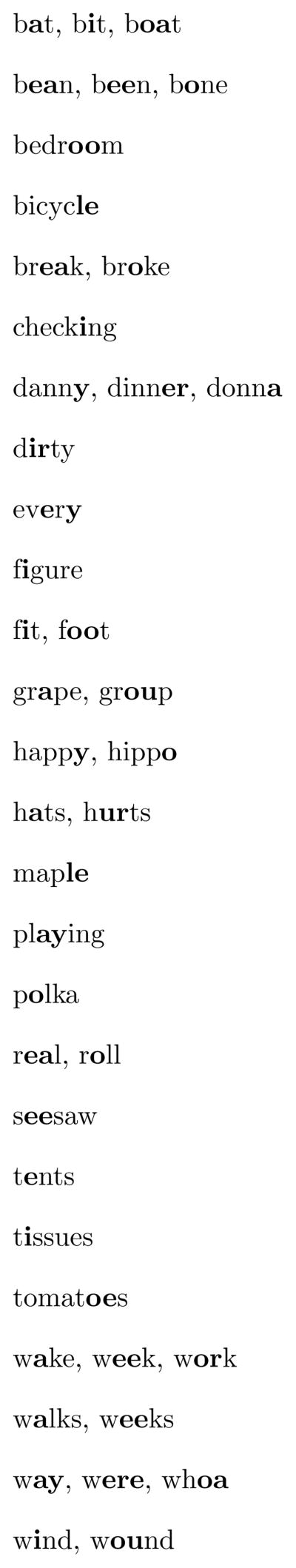
Contents of one of the super-categories found by a model with a strong bias toward a smaller lexicon (α_L = 10). The sounds identified as belonging to the super-category are highlighted in bold. Multiple orthographic forms are listed next to each other if tokens of that lexical item correspond to more than one word. Many of these lexical items are minimal pairs that the model mistakenly categorizes together.

General discussion

In this paper we investigated how higher-level lexical knowledge can contribute to lower-level phonetic category learning by creating a lexical-distributional model of simultaneous phonetic category and word learning. Under this model, learners are not assumed to have knowledge of a lexicon a priori, but are assumed to begin learning a lexicon at the same time they are learning to categorize individual speech sounds, allowing them to take into account the distribution of sounds in words. Across several simulations, phonetic categorization performance was shown to be significantly better in a lexical-distributional model than in distributional models. These results provide support for the hypothesis that the words infants segment from fluent speech can provide useful constraints to guide their acquisition of phonetic categories, as well as for the more general idea that complex systems incorporating multiple levels of structure are not best acquired by focusing on each level in turn, but rather by considering multiple levels simultaneously.

Here we situate the idea of interactive learning in a broader context. We first examine the limitations of our modeling framework and the extent to which those limitations affect the conclusions we can draw. We then consider the role of minimal pairs and discuss ways in which the model’s behavior in dealing with minimal pairs can explain human behavior from artificial language learning experiments. Finally, we discuss the implications of our findings for theories of sound and word learning and for category learning more generally.

Model assumptions

Our lexical-distributional model was built to illustrate how feedback from a developing word-form lexicon can improve the robustness of phonetic category acquisition. A hierarchical nonparametric Bayesian framework was chosen for implementing this interactive model because it allows simultaneous learning of multiple layers of structure, with information from each layer affecting learning in the other layer in a principled way. However, there were several simplifications that we used when creating our corpus that restrict the extent to which we can draw conclusions from these results. One simplification, the lack of phonotactics, actually led to decreased learning performance, and we address this issue in the next section. Here we examine in detail the role of three other simplifying assumptions: the use of only two acoustic dimensions, the reliance on Gaussian distributions of sounds, and the omission of contextually conditioned variability.

In constructing our corpora we assumed that learners attend to only two acoustic dimensions, corresponding to the first and second formants, when learning vowel categories. Real speech input has rich acoustic cues, and vowels have been shown to differ reliably along dimensions such as duration (Vallabha et al., 2007) and formant trajectories (Hillenbrand, Clark, & Nearey, 2001). In limiting ourselves to two dimensions we may have overestimated the difficulty of the learning problem. Vowel categories exhibit substantial overlap when viewed in two dimensions, but additional dimensions may lead to greater separation between categories. Given that our lexical-distributional learning algorithm works well on just two acoustic dimensions, it is likely that the same strategy would succeed when additional informative dimensions are taken into consideration. However, distributional learning algorithms may also produce better results when given richer cues that help separate overlapping categories. At this point our results should not be taken as evidence that distributional learning is impossible, but rather that an interactive learning strategy can improve the learning outcome on categories that pose a challenge for distributional learning. Both distributional learning and interactive learning, as described in Appendices A and B, can be implemented for arbitrary numbers of dimensions, and this will allow the issue of the number of relevant dimensions to be examined in detail in future work.

A second simplifying assumption present in our models and corpora was that sounds fall into Gaussian distributions along the relevant phonetic dimensions. While this same assumption has been made in previous models of phonetic category acquisition (McMurray et al., 2009; Vallabha et al., 2007), it is not likely to be true in real speech data. Gaussian mixture models have shown substantial difficulty in cases where they were trained directly on acoustic vowel measurements (de Boer & Kuhl, 2003; Dillon et al., 2013). The fact that acoustic values in our corpora were sampled directly from Gaussian distributions is likely to have improved learning performance in all three models. Because it affected all three models equally, this simplification should not have affected the comparison across models, but in future work it will be important to replicate these results using actual acoustic values from speech corpora.

More importantly, if real speech data exhibit non-Gaussian distributions of sounds and learners eventually acquire knowledge of these distributions, then learning algorithms need to be extended to consider non-Gaussian distributions in their hypothesis space. Vallabha et al. (2007) proposed one potential method by which models might learn non-Gaussian categories, and Gaussian assumptions have also been relaxed within the framework of neural network models of phonetic learning (Behnke, 1998; Gauthier, Shi, & Xu, 2007). The extent to which such proposals can be integrated within a hierarchical learning framework remains an interesting question for future research. One possibility would be to incorporate more flexible function learning algorithms (e.g. Griffiths, Lucas, Williams, & Kalish, 2009), but relaxing the Gaussian assumption makes the search space of hypotheses considerably larger, presenting a challenge for probabilistic frameworks. In this case having additional constraints from lexical structure might become even more critical.

A third simplification was the lack of contextual variation in our training corpora. In these corpora acoustic values for each sound were sampled independently of surrounding sounds. This contrasts with actual speech data, where acoustic characteristics of sounds change in a context-dependent manner. These context-dependent changes come from coarticulation with neighboring sounds (e.g., Hillenbrand et al., 2001) and phonological alternations (e.g., Pegg & Werker, 1997) and lead to patterns of complementary distribution, in which distinct acoustic realizations of phonemes occur consistently in distinct phonological contexts. This means that the data given to our models satisfied the idea that sounds were sampled independently of their context, but real speech data would not satisfy this assumption. Similarly, schwa vowels were not included in our simulations, as they are not present in the CMU pronouncing dictionary and were also not included in the production study by Hillenbrand et al. (1995). In real speech data these would arise through phonological processes of vowel reduction. At a minimum, the presence of schwas would require learners to recover one additional vowel category, but one might also expect learners to notice that reduced and unreduced vowels alternate based on stress assignment.

Phonological processes that operate across word boundaries can potentially cause sounds to appear interchangeably in the same set of words, and this would allow learning to proceed through a mechanism similar to our proposed model, as suggested by Martin, Peperkamp, and Dupoux (2013). However, phonological processes that affect primarily word-internal sounds pose a problem for our model. A lexical-distributional learner hearing reliable differences between sounds in different words would be likely to erroneously assign coarticulatory variants of the same phoneme to different categories, having no other mechanism to deal with context-dependent variability. This means that omitting context-conditioned variability from the corpus is likely to have benefitted the lexical-distributional model. In contrast, it is not obvious that the presence or absence of contextually conditioned variability would affect learning performance in a distributional learning model. Because of this, it is not clear which type of model would perform better on training data that incorporate contextually conditioned variability.

The lexical-distributional model’s predicted difficulty with coarticulation and allophony points to an inherent confound in language input. Lexical structure, which we have shown to be useful for separating overlapping categories, is confounded with context-dependent phonological variability. Consistent acoustic differences across words can arise either because the words contain different sounds or because the words contain the same sound in different phonological environments. The lexical-distributional model only considers one of these potential causes for systematic acoustic variability across words.

Dillon et al. (2013) have begun to address this problem of contextually conditioned variability, proposing a generative framework in which a phoneme’s pronunciation varies depending on the identities of neighboring sounds. They analyzed this learning problem mathematically and built a model in which phonemes are represented as context-dependent mixtures of Gaussians. Their model showed promising learning performance when trained on formant values measured from vowel productions. Although their model has not yet been mathematically combined with ours, it fits nicely into the theoretical framework of interactive lexical-distributional learning. White et al. (2008) have shown that infants can detect transitional probability patterns that reflect phonological alternations at eight months of age, during the same period when they are segmenting words and learning about phonetic categories. These data suggest that in addition to segmenting and categorizing words, young infants are sensitive to dependence of pronunciation on phonological context, and are learning all three aspects of linguistic structure simultaneously.

These considerations emphasize the fact that this model provides only a starting point for characterizing how children learn sounds and words. Several issues need to be addressed before the model can be applied to realistic corpus data, the most important of which is adding a mechanism to account for contextually conditioned variability. Nevertheless, interactive learning across different layers of linguistic structure is likely to remain a key component even as the model is scaled up to deal with more realistic corpus data.

The role of minimal pairs

Phonetic analyses, such as distributional learning, identify sound categories by analyzing the clustering of these sounds according to their acoustic properties. In contrast, phonological analyses concern the distributions of sounds with respect to the sound contexts in which they occur (Chomsky & Halle, 1968; Jakobson & Halle, 1956; Trubetzkoy, 1939). As we have shown here, distributional phonetic analyses may be inadequate for acquisition of overlapping phonetic categories. The interactive lexical-distributional learning model that we have proposed instead is similar to the types of phonological analyses used in theoretical linguistics in that it takes into account the context in which sounds appear. However, our model’s predictions diverge in interesting ways from the inferences that are typically drawn by theoretical linguists on the basis of contextual patterns.

One key phenomenon exploited in phonological analyses is the existence of minimal pairs, which serve as evidence that two superficially similar sounds are actually members of different categories. For example, bad and bed constitute a minimal pair, two distinct words that differ from each other only by a single phoneme. A linguist analyzing English, knowing that these are different words, can infer that /æ/ and /ε/ are functionally different sounds in the language. In our model, minimal pairs are treated in the opposite way. The model, having no access to word meanings, mistakenly interprets items from minimal pairs as tokens of the same word. These mistakes in lexical categorization lead to mistakes in phonetic category learning, as the wide acoustic variability across tokens in merged lexical items lead the model to hypothesize extra phonetic categories with a high degree of acoustic variability. That is, the lexical-distributional model misinterprets minimal pairs like bad and bed as different tokens of the same word and as a consequence, it mistakenly creates an extra category that can accommodate acoustic values corresponding to both /æ/ and /ε/.

Although linguists use minimal pairs to identify sound contrasts, young learners may not use minimal pair based strategies on a large scale in acquiring their first language. Minimal pair analyses crucially rely on learners’ knowledge that the words have different meanings. If meanings are not known, learners can interpret similar-sounding acoustic tokens such as bad and bed as tokens of the same word. The role of minimal pairs in phonetic category acquisition therefore critically depends on the extent to which young infants have access to associations between form and meaning. Children do appear to know some minimal pairs at a young age, but may not have sufficient vocabulary knowledge to support large-scale minimal pair based learning, making it unlikely that early sound category acquisition relies primarily on information from minimal pairs (Charles-Luce & Luce, 1990, 1995; but see Bergelson & Swingley, 2012; Coady & Aslin, 2003; Dollaghan, 1994). Instead, a good deal of recent theoretical, empirical, and computational work has demonstrated that non-minimal pairs might provide cues for phonetic learning during language acquisition (Feldman, Myers, White, Griffiths, & Morgan, 2013; Martin et al., 2013; Swingley & Aslin, 2007; Swingley, 2009; Thiessen, 2007, 2011; Thiessen & Pavlik, 2013).

If infants were using a minimal pair based strategy for acquiring sound categories, we should expect to find consistent evidence that pairings of words and objects are helpful for separating similar sound categories. While some facilitation from word-object pairings has been shown for nine-month-old infants (Yeung & Werker, 2009), the opposite has been found in experiments that use the switch task (Stager & Werker, 1997). In this task, infants are habituated to one or more word-object pairings; during test the pairings are changed so that familiar objects are paired with novel labels. Success on the task is indicated by dishabituation to novel pairings, as indicated by longer looking times. Stager and Werker (1997) found that 14-month-old infants fail to notice when minimally different object labels bih and dih are switched. This pattern has been replicated using other types of contrasts, such as a voicing contrast, a place contrast, and a two-feature voicing and place contrast (Pater, Stager, & Werker, 2004). Infants succeed in discriminating the same labels when no potential referents are given (Stager & Werker, 1997), when the referential context is made clear to them (Fennell & Waxman, 2010), or when the test paradigm is simplified (Yoshida, Fennell, Swingley, & Werker, 2009), suggesting that task difficulties are masking their sensitivity to phonetic detail.

Critically, children’s poor performance in the switch task appears only in minimal pair contexts: 14-month-olds succeed at the task with the easily distinguishable labels lif and neem (Werker, Cohen, Lloyd, Casasola, & Stager, 1998). It thus provides a method for identifying which type of familiarization stimuli best support children’s ability to distinguish between words. Thiessen (2007) used the switch task to specifically investigate the effects of word context on children’s use of phonetic contrasts. He replicated the basic finding, showing that 15-month-old infants fail to notice when minimal pair object labels (in this case, daw and taw) are switched. He then added two additional object-label pairings to the habituation phase: either dawbow and tawgoo, or dawgoo and tawgoo. Infants who heard the words dawbow and tawgoo as additional object labels during habituation discriminated between daw and taw during test, but this facilitation did not occur when the additional object labels were dawgoo and tawgoo. These results suggest that facilitation was related to the degree of difference between the two extra familiarized words. The same qualitative pattern has been found using syllable-final consonant contrasts as well (Thiessen & Yee, 2010).

The facilitation observed in non-minimal pair contexts is not specific to the switch task, but has been found in other experimental paradigms as well. Feldman et al. (2013) obtained similar results with adults in a non-referential task. In their experiment, sounds ranging along a vowel continuum from tah to taw were embedded in pseudowords guta and lita. One group of participants heard all tah and taw sounds interchangeably in both words, whereas the other group heard the tah half of the continuum consistently in one word and the taw half of the continuum consistently in the other word. Participants who heard tah and taw in different word contexts were more likely to assign these stimuli to different categories at the end of the experiment than participants who heard the sounds interchangeably. Words without referents similarly help 15-month-old infants perform better on the switch task (Thiessen, 2011) and lead to better sound differentiation by 8-month-old infants (Feldman et al., 2013). These findings extend Thiessen’s (2007) findings to novel paradigms, contrasts, and age groups, suggesting that the results are not tied to a specific laboratory task but instead reflect general principles of sound category learning. The acquisition and use of sound contrasts is facilitated when the sounds are heard in distinct lexical contexts.

Results from these experiments are opposite of what would be predicted if learners were using minimal pairs as their primary basis for acquiring phonemes. Minimal pairs like dawgoo and tawgoo or gutah and gutaw do not facilitate distinctions between sounds, whereas non-minimal pairs like dawbow and tawgoo or gutah and litaw do facilitate these distinctions. This pattern instead suggests that learners are attending to acoustic differences between the words in which sounds appear. When two sounds appear consistently in distinct lexical contexts, they are likely to represent different categories, whereas if the sounds appear interchangeably in the same set of lexical contexts, they are more likely to belong to the same phonetic category. Reliance on word-level information has been incorporated into Thiessen and Pavlik’s (2013) model as an a priori assumption, but our model predicts that this behavior arises as a simple consequence of simultaneous learning of phonetic categories and lexical items. Here we illustrate how our model can explain data from this type of experimental setting, using a simple synthetic dataset to show that learners’ behavior in these experiments falls directly out of our model.

We mimic the experimental stimuli from Feldman et al. (2013) using four phonetic categories labeled A, B, C, and D, shown in Figure 8a. The category means are located at −5, −1, 1, and 5 along an arbitrary phonetic dimension, and all four categories have a variance of 1. Because the means of categories B and C are so close together, being separated by only two standard deviations, the overall distribution of tokens in these two categories is unimodal. Categories B and C play the role of the similar sounds in our simulations, and categories A and D are used to create the different lexical contexts.

Figure 8.

Simple synthetic data with two overlapping categories, demonstrating the treatment of minimal pairs. Data are shown as (a) generated, (b) recovered by the distributional model, (c) recovered by the lexical-distributional model from a minimal pair corpus, and (d) recovered by the lexical-distributional model from a corpus without minimal pairs.

Two simple corpora were constructed, one corresponding to each experimental condition. Both corpora contained the same set of 1600 phonetic values, consisting of 400 tokens drawn randomly from each of the four Gaussian phonetic categories. The corpora differed from each other in the distribution of these phonetic values across lexical items. The lexicon of the first corpus contained no disambiguating information about categories B and C. It was generated from four lexical items, with identities AB, AC, DB, and DC. Each lexical item was repeated 200 times in the corpus for a total of 800 word tokens. In this corpus, Categories B and C appeared only in minimal pair contexts, since both AB and AC, as well as both DB and DC, were words. The second corpus contained disambiguating information about categories B and C. This corpus was identical to the first except that the acoustic values representing the phonemes B and C of words AC and DB were swapped, converting these words into AB and DC, respectively. Thus, the second corpus contained only two lexical items, AB and DC, and there were now 400 tokens of each word. Categories B and C did not appear in minimal pair contexts, as there was a word AB but no word AC, and there was a word DC but no word DB. We refer to the first corpus as the minimal pair corpus and the second as the informative corpus.

Simulations used parameters α_C = α_L = 1, m₀ = 0, ν₀ = 0.001, and S₀ = 0.001. The distributional model was trained on the 1600 acoustic values. Distributional information correctly separated out categories A and D, but it was insufficient to distinguish categories B and C from each other (Figure 8b). The lexical-distributional model was trained separately on each of the two corpora. As shown in Figure 8c, the model merged categories B and C when trained on the minimal pair corpus. Merging the two categories allowed the learner to condense AB and AC into a single lexical item, and the same happened for DB and DC. Because the distribution of these sounds in lexical items was identical, lexical information could not help separate the categories. In contrast, the lexical-distributional model was able to use the information contained in the lexicon in the informative corpus to successfully disambiguate categories B and C (Figure 8d). This occurred because the model could categorize words AB and DC as two different lexical items simply by recognizing the difference between categories A and D, and could use those lexical classifications to notice small phonetic differences between the second phonemes in these lexical items.

These patterns parallel the experimental results described above. When similar sounds are heard in different word contexts, they are more likely to be assigned to different categories. Minimal pairs may be useful when a learner knows that two similar sounding tokens have different referents, but they pose a problem in this model because the model hypothesizes that similar sounding tokens represent the same word. The resemblance between human and model behavior suggests that participants’ reliance on word-level information in these experiments can be explained through an interactive learning strategy in which participants simultaneously learn to categorize both sounds and words.

The close resemblance between model behavior and human data raises the possibility that the model’s trouble with minimal pairs reflects a real difficulty that learners face during phonetic category acquisition. That is, human learners might sometimes misinterpret members of minimal pairs as tokens of the same word. This resembles an account given by Sebastián-Gallés and Bosch (2009) to explain patterns of sound category acquisition in Spanish-Catalan bilinguals. Infants raised in Spanish-Catalan bilingual environments temporarily lose the ability to discriminate [o] and [u] around eight months of age, despite the fact that these sounds are contrastive in both Spanish and Catalan. Sebastián-Gallés and Bosch suggest that these infants may be confused by the large number of cognates between the two languages. They give the example of the word ‘boat’, pronounced /barko/ in Spanish and /barku/ in Catalan, to illustrate the type of evidence that could cause such confusion. If learners have not yet entirely succeeded in separating the two languages, hearing a high number of such cognates could lead them to erroneously conflate [o] and [u].

While this type of explanation might play a role in explaining some aspects of learners’ developmental trajectories, and although learners may not rely heavily on minimal pairs for distinguishing similar phonemes, there are also several reasons to think that minimal pairs do not pose a significant problem in most phonetic learning situations. The problem of minimal pairs arises in our model because of a simplifying assumption: Our model incorporates no phonotactic regularities into its lexicon. The English lexicon contains more minimal pairs than would be expected on the basis of this assumption of no phonotactics. For example, counting the number of pairs of distinct phonemic forms in the CHILDES parental frequency count (Li & Shirai, 2000) that differ by exactly one phoneme yields 29,767 minimal pairs. To explore the extent of the mismatch between these corpus values and our model’s assumptions, we created a series of artificial lexicons that matched the actual distribution over word lengths, in which phoneme sequences were constrained by observed phoneme frequencies but not by any phonotactics. On average, these lexicons contained 9,199 minimal pairs, a substantially lower number than are actually present in the corpus.

It is important to note that simply adding more training data does not solve the lexical-distributional model’s problem with minimal pairs. Using larger training corpora actually makes the problem worse, because the difference between the predicted and observed number of minimal pairs becomes more statistically reliable as corpus size increases. Instead, improving learning performance requires that the learner’s assumptions match the characteristics of the linguistic input.

The lack of phonotactics was a problem for our model, but it may not be a problem for young infants. Infants appear to have knowledge of phonotactics by nine months (Jusczyk, Luce, & Charles-Luce, 1994) and perhaps even as early as six months (Molina & Morgan, 2011). Knowledge of phonotactics can improve performance by assigning higher probability to phoneme sequences that occur frequently in the lexicon, raising the probability of generating the same consonant frame more than once. Crucially, phonotactic constraints appear to be acquired in parallel with sound and word categories, suggesting that infants do not make the same simplifying assumption regarding phonotactics as was present in our model.

Other types of information are also available to help infants separate similar sounding words. For example, semantic information about words can potentially help infants separate minimal pairs in their lexicon. Although most mappings between words and objects are thought to be learned later in development (e.g. Woodward, Markman, & Fitzsimmons, 1994; Werker et al., 1998), 9-month-old infants can use cooccurences between sounds and objects to constrain phonetic category learning (Yeung & Werker, 2009). Recent findings also suggest that word-object mappings may be available to infants earlier than was previously believed (Bergelson & Swingley, 2012). This early knowledge might give learners a way to separate very common sets of minimal pairs, perhaps even supporting something parallel to the improved performance that has been observed in the switch task with familiar words in older infants (Fennell & Werker, 2003). Finally, if infants are sensitive to phrase-level information, they may be able to use the phrases to separate acoustically similar words, parallel to the way in which they can use words to separate acoustically similar sounds. That is, hearing bed and bad in distinct sentential contexts can provide evidence that these are tokens of different words. These considerations suggest that a number of strategies are potentially available to infants for avoiding the challenges posed by minimal pairs, and that more realistic models of acquisition would not necessarily face the problem encountered by our model.

Learning a prior distribution over lexical items

Lexical-distributional learning differs from many previously proposed statistical learning algorithms in that it is based on a hierarchical model. Hierarchical models allow simultaneous learning of specific items (e.g., the pronunciations of individual words in the lexicon) and information about general characteristics of items (e.g., the pronunciations of phonetic categories that tend to occur in a variety of words). General knowledge that constrains lower levels of learning is often referred to as overhypotheses (N. Goodman, 1955; Colunga & Smith, 2005), and in our model knowledge of phonetic categories constitutes a type of Bayesian overhypothesis (Kemp, Perfors, & Tenenbaum, 2007; Perfors, Tenenbaum, & Wonnacott, 2010). Knowledge of phonetic categories benefits learners by allowing them to predict what sort of variability a new lexical item is likely to exhibit on the basis of only a few acoustic tokens. This shifts the focus of learning to the word level: knowledge of sounds is nothing more than a type of general knowledge about words.

Defining phonetic categories as a prior distribution over the forms of lexical items means that learners can obtain an estimate of phonetic category parameters by computing statistics over the items in their hypothesized lexicon. Similar approaches to phonetic learning have recently been proposed in the automatic speech recognition community as well (Jansen & Church, 2011). This contrasts with distributional learning models in which statistics are computed directly over tokens from the corpus, but it parallels approaches in other linguistic domains. For example, the idea of computing statistics over the lexicon has been proposed for unsupervised learning of phonotactics (Hayes & Wilson, 2008) and morphology (Goldwater, Griffiths, & Johnson, 2006; Goldwater et al., 2011). Computing statistics over lexical items is appropriate when the domain to be learned is a component of the prior distribution over lexical items, and this is a reasonable assumption in all of these cases.

The prior distribution over lexical items is likely to have many components, with phonetic categories, phonotactics, and morphology all providing constraints on lexical structure. These provide potential ways to extend the model in future work. For example, our model mistakenly merged lexical items when trained on the English lexicon, and languages with richer morphological structure would likely present an even greater challenge in this respect. In Spanish, verb conjugation patterns like quiero ‘want-1sg’ and quiere ‘want-3sg’ produce sets of minimal pairs that all share the same set of vowels. Similar patterns are found in languages with templatic morphology, such as Arabic and Hebrew. One potential solution would be to directly model morphology as part of the prior distribution over words (cf. M. Johnson et al., 2007). Although it is not yet clear at what point this type of pattern becomes available to infants, as sensitivity to morphological patterns has been found only at 11 months in French-learning infants (Marquis & Shi, 2009) and not until 15–18 months in English-learning infants (Mintz, 2004; Santelmann & Jusczyk, 1998; Soderstrom, White, Conwell, & Morgan, 2007), it is possible that morphology also interacts with phonetic learning.

Finally, it is possible that children need to learn the structure, as well as the content, of the prior distribution over lexical items. For example, learners might infer that lexical items are composed of sequences of phonetic categories by examining the words in their developing lexicon. Our implementation of the lexical-distributional model assumes the form of this prior distribution is known in advance, but our broader theoretical framework is potentially compatible with the idea that representations such as phonetic categories emerge during development, as a result of learners observing statistical regularities across lexical items. Research has begun to formalize structure learning problems using Bayesian methods (e.g. Kemp & Tenenbaum, 2008), and it will be interesting to apply those methods to investigate which additional aspects of the prior distribution over lexical items might be learned from linguistic input.

Relation to process level models

Our model addresses Marr’s (1982) computational level and embodies the idea of rational analysis (Anderson, 1990), providing a formal analysis of the computational problem faced by learners and the statistical solution to that problem. The assumption behind this type of modeling strategy is that infants are solving a statistical inference problem when they acquire language, and that identifying which problem they are solving can give us clues to the types of strategies that are likely to be used. We analyzed the learning problem that arises when sounds are organized into words, comparing this to the learning problem that arises when sounds are uttered in isolation, and our more realistic assumptions led to better model performance. This is one example of how formal analyses can lead to principled hypotheses about learning strategies that might be used during language acquisition.

However, because it is specified at the computational level, our model does not directly address the question of which representations and processes are involved in interactive learning of sounds and words. With regard to processes, using a Bayesian framework limits our ability to take into account the time course of development. Our use of a Gibbs sampler in this paper is certainly not meant to suggest that children use a batch learning algorithm when acquiring language. Furthermore, our simulations reflect the learning outcome that can be achieved by an ideal learner at a single time point using a given effective corpus size, but it is not clear how this maps onto any particular time point in children’s development.

One way to look at learning trajectories across development might be to examine the learning outcome in response to varying amounts of training data, running several simulations that are trained on different corpus sizes. This approach has been used in previous work (e.g. Kemp & Tenenbaum, 2008), yielding predictions about qualitative changes in learners’ representations. This strategy is appealing in that it requires no additional machinery aside from the Bayesian model itself. However, it also has potential drawbacks, in that it necessarily assumes that learners are optimal at every time during development and also gives no account of how learners update their beliefs from one time point to the next. For these reasons, it is worth considering ways in which Bayesian computations might be implemented in an incremental fashion.

There is a growing literature on process level models that might support Bayesian computations (Kwiatkowski, Goldwater, Zettlemoyer, & Steedman, 2012; Pearl, Goldwater, & Steyvers, 2011; Sanborn et al., 2010; Shi, Griffiths, Feldman, & Sanborn, 2010). Learners encounter speech as it unfolds in time, and thus it seems likely that they would use an incremental algorithm to update their beliefs about linguistic structure. One possible algorithm is particle filtering (Sanborn et al., 2010), a sequential Monte Carlo method in which new data points are assigned to categories probabilistically as they occur. In the lexical-distributional model, learners would categorize each sound and word based on their current beliefs about the phonetic category inventory and lexicon. Those category assignments would then contribute to the prior distribution for future assignments. However, learners would not have an opportunity to revise category assignments for previous sounds. This algorithm is guaranteed to converge to the posterior distribution over category assignments if learners keep track of many hypothesized category assignments for each sound, but it loses this guarantee if learners are limited in the number of hypotheses they store in memory. A second type of incremental algorithm, local MAP (Anderson, 1990; Sanborn et al., 2010; Pearl et al., 2011), is similar to a particle filter in many ways, but each new datapoint is assigned deterministically to the category that has highest posterior probability given the previous assignments. Although this algorithm does not have convergence guarantees, empirically it outperforms even a more powerful batch sampling algorithm in some cases, such as word segmentation under a unigram language model (Goldwater et al., 2009; Pearl et al., 2011). A third variant of incremental learning is online variational inference (Kwiatkowski et al., 2012), which, instead of sampling category assignments or assigning points to the highest probability category, tracks the expectations (under the posterior) of the category assignments. One way to view this is as if each data point is partially assigned to several different categories, with the amount of fractional assignment depending on each category’s probability of having generated that data point. As in the previous two algorithms, category assignments are made as each data point is observed and cannot be revised afterward; thus all three of these algorithms can potentially provide incremental implementations of Bayesian computations. A final possibility, explored by Pearl et al. (2011), is that learners do revise old hypotheses, but to a lower degree than would be predicted by batch learning algorithms. All of these proposals have shown promising performance in comparison to batch learning algorithms, and they provide frameworks for beginning to explore implementations for interactive learning that are incremental, computationally tractable, and robust.

It is also important to consider representations that might support the computations described in this paper. While it is possible that listeners do store and update parameters associated with probability distributions, our use of explicit probability distributions to represent phonetic categories is not meant to be taken as a theoretical claim. One alternative proposal that has received a good deal of attention is that knowledge of words and sounds is represented through stored exemplars (K. Johnson, 1997; Pierrehumbert, 2001). Listeners appear to retain detailed knowledge of speaker characteristics in word recognition tasks (Goldinger, 1996), and sounds in frequent words are more prone to reduction or lenition than sounds in infrequent words (Bybee & McClelland, 2005; Gahl, 2008). This suggests that phonetic knowledge is stored separately for each word and is also sensitive to non-linguistic characteristics of situations in which those words appear. Exemplar models explain these findings by proposing that listeners’ perception uses stored examples of individual sounds, words, or utterances they have heard, rather than using a stored representation that abstracts away from those examples.

Exemplar models are often viewed as being incompatible with traditional ideas about sound category structure (e.g. Port, 2007). Whereas most theories assume that learners extract generalizations about sounds and words, in exemplar models these generalizations are unnecessary during learning and are epiphenomenal during perception. This poses a potential challenge for the assumption in our lexical-distributional model that learners extract sound and word categories based on distributions in the input. However, while it is clear that exemplar models are inconsistent with representations that correspond to sound and word categories, it is less straightforward to determine whether they are consistent with the existence of categories at Marr’s (1982) computational level of analysis. Probabilistic computations can often be approximated using samples from the relevant distributions, and because of this, exemplar models can be used to approximate at least some types of Bayesian models. If exemplar models can be used to approximate lexical-distributional learning, then they can be thought of as simply another way of implementing our computational level model.

It is not yet clear whether exemplar models can provide a plausible approximation to our lexical-distributional learning model. Ashby and Alfonso-Reese (1995) demonstrated that for categorization tasks, exemplar models provide a way of carrying out nonparametric density estimation. Learners are assumed to store labeled exemplars belonging to a category. They can then assign new exemplars to categories on the basis of the similarity between those new exemplars and previously encountered exemplars. This can provide a way to implement the computation of category assignments given in Equation 2, but it falls short of providing an implementation for our entire model because it requires the presence of labeled exemplars.

Shi et al. (2010) proposed a second way in which exemplar models can approximate Bayesian computations: If stored exemplars correspond to samples from the prior distribution over hypotheses, then importance sampling can be used to estimate the posterior distribution. This simply requires that exemplars be weighted according to a similarity function that is proportional to the likelihood. It is not immediately obvious how to apply this method to our lexical-distributional model, as each hypothesis in our model consists of a phonetic category inventory, a lexicon, and a set of category labels for each sound and word in the corpus. Learners would need to obtain a set of exemplars representing samples from the prior distribution over these complex hypotheses, and there is not an obvious way that they could obtain such a sample through experience. Despite the fact that our model does not meet the requirements for these specific parallels between Bayesian and exemplar models, it is possible that future work will reveal a framework in which something similar to an exemplar model can be used to implement interactive learning of sounds and words.

Thiessen and Pavlik (2013) provide a starting point for thinking about how this might work, proposing an exemplar-based framework for implementing distributional learning. Although their model is unable to capture the idea that sounds constitute higher level knowledge that can be generalized across words (McQueen, Cutler, & Norris, 2006; White & Aslin, 2011; but see Thiessen & Yee, 2010), they do account for data from Thiessen (2007) by treating word contexts as acoustic dimensions. It will be interesting to explore how this type of framework can be extended to represent knowledge at multiple layers of generality, and to what extent this type of hierarchical structure can emerge from the input that children receive.

Category learning in language and other domains

Our model is built around sound and word learning, but it is potentially applicable to other domains in language and cognition as well. When acquiring language, infants need to learn multiple layers of linguistic structure. Sounds are organized into words, words combine to form sentences, and sentences convey meaning in real-world contexts. Investigations of statistical learning often consider each domain in isolation or assume that acquisition proceeds sequentially (e.g. Saffran & Wilson, 2003; Graf Estes et al., 2007; Christiansen, Onnis, & Hockema, 2009). Contrary to this assumption, our simulations suggest that statistical learning is most effective when dependencies between domains are taken into account. Recent models of language acquisition have begun investigating the outcome of interactive learning in a variety of linguistic domains, such as word boundaries and word meanings (Jones, Johnson, & Frank, 2010), word meanings and syntactic structure (Maurits, Perfors, & Navarro, 2009), or syntactic and semantic structure (Kwiatkowski et al., 2012), each time with promising results. It is important to identify interactions between levels of linguistic structure because they can qualitatively change how we conceptualize the learning problem. For example, if infants are distributional learners, then research should be focused on determining how they solve the problem of overlapping categories, but if they are interactive learners we might instead focus on questions about how they deal with similar sounding words.

More broadly, one might hypothesize that perceptual categories in general correspond to higher level knowledge that helps people learn relationships among objects in the world. For example, Kemp, Shafto, Berke, and Tenenbaum (2007) proposed that perceptual similarity between objects could be used to detect whether those objects were likely to participate in similar types of causal relationships. In N. D. Goodman, Mansinghka, and Tenenbaum (2007), perceptual categories were inferred directly based on their role in causal structure, and Kemp, Tenenbaum, Griffiths, Yamada, and Ueda (2006) used a similar approach to learn categories from relational data. Lake, Salakhutdinov, Gross, and Tenenbaum (2011) proposed a hierarchical framework for learning to recognize novel handwritten characters, and object recognition in general has benefitted from an approach in which the prior distribution is defined in terms of reusable parts (e.g. Sudderth, Torralba, Freeman, & Willsky, 2008). Other work has explored how learning multiple categories simultaneously can affect the resulting category representations (Gureckis & Goldstone, 2008; Canini et al., 2010; Canini & Griffiths, 2011). In each of these cases, members of each category shared some level of surface similarity, but categories were also used as building blocks for various types of higher level structures. Top-down information from these higher level structures provided a cue that learners could use to recover the underlying categories, supplementing the bottom-up similarity structure. Combining information in this way is an optimal learning strategy for learners who live in a world with multiple layers of structure.

Considering the interaction between different sources of information becomes even more important as we go beyond the artificial stimuli typically used in studies of category learning. An important set of constraints guiding human category learning comes from explicit knowledge about the world. People are strongly affected by this knowledge when learning new categories, with categories that are consistent with prior knowledge being easier to learn. However, the relevant knowledge is extremely diverse, with experiments demonstrating the effects of intuitions about the factors that influence the inflation of balloons (Pazzani, 1991), the properties of different types of buildings (Heit & Bott, 2000), the definition of honesty (Wattenmaker et al., 1986), and the properties of vehicles (Murphy & Allopenna, 1994). Only a small number of computational models of knowledge effects in category learning exist (Rehder & Murphy, 2003; Heit & Bott, 2000), and these models treat prior knowledge as a fixed quantity that is exploited by the learner. Understanding how people build complex theories about the world around them at the same time as learning the concepts on which those theories are built is a major challenge for accounts of human category learning, and a place where the insights obtained by studying language acquisition may be relevant.

Conclusion

Infants learn multiple levels of linguistic structure, and it is often implicitly assumed that these levels of structure are acquired sequentially. This paper has instead investigated the optimal learning outcome in an interactive system using a nonparametric Bayesian framework that permits simultaneous learning at multiple levels. Our results demonstrate that information from words can lead to more robust learning of phonetic categories, providing one example of how such interaction between domains might help make the learning problem more tractable.

Appendix A

Infinite mixture model

We use x_i to represent individual sounds in the corpus and z_i to denote a category label for an individual sound x_i. This category label z_i indexes directly into the phonetic category inventory. N represents the total number of sounds in the corpus, and c denotes the index of a phonetic category in the phonetic category inventory. Parameters μ_c and Σ_c represent the mean and covariance of category c and are assumed to be drawn from a prior distribution G_C, a normal inverse Wishart distribution which plays the role of the base distribution in the Dirichlet process. Using this notation, the generative model for our distributional model is

$$\begin{array}{lll}\hfill & {\mathrm{\sum }}_c~IW({\nu }_0,S_0),\hfill & c=\mathrm{1..}\infty \hfill \\ G_C:\hfill & \hfill & \hfill \\ \hfill & {\mu }_c~N(m_0,\frac{{\mathrm{\sum }}_c}{{\nu }_0}),\hfill & c=\mathrm{1..}\infty \hfill \\ \hfill & z_i~DP({\alpha }_C,G_C),\hfill & i=\mathrm{1..}N\hfill \\ \hfill & x_i~N({\mu }_{z_i},{\mathrm{\sum }}_{z_i}),\hfill & i=\mathrm{1..}N\hfill \end{array}$$

Inference in the distributional model uses a collapsed Gibbs sampler, integrating over the means μ_c and covariances Σ_c of phonetic categories. Minus symbols in subscripts are used to denote the exclusion of particular components; for example, z_−i, is used to denote all category labels except z_i. Each sound x_i is given a new category assignment z_i according to Bayes’ rule, based on other sounds’ current category assignments z_−i

$$p(z_i=c\mid x_i,z_{-i})\propto p(x_i\mid z_i=c,z_{-i})p(z_i=c\mid z_{-i})$$ (3)

The prior distribution p(z_i = c|z_−i) is defined by the Dirichlet process to be

$$\begin{array}{l}\frac{n_c}{{\displaystyle \sum _c}{n}_c+{\alpha }_C}\text{for}\text{existing}\text{categories}\\ \frac{{\alpha }_C}{{\displaystyle \sum _c}{n}_c+{\alpha }_C}\text{for}\mathrm{a}\text{new}\text{category}\end{array}$$ (4)

where n_c is the number of times the phonetic category c has been used previously in the corpus. The likelihood p(x_i|z_i = c, z_−i) is computed by integrating over all possible means and covariance matrices for the category to obtain a multivariate t-distribution,

$$\frac{\mathrm{\Gamma }\left(\frac{{\nu }_c+1}{2}\right)}{\mathrm{\Gamma }\left(\frac{{\nu }_c+1-d}{2}\right)}{\left|\pi S_c\left(\frac{{\nu }_c+1}{{\nu }_c}\right)\right|}^{-\frac{1}{2}}{\left(1+{(x_i-m_c)}^T{\left[S_c\left(\frac{{\nu }_c+1}{{\nu }_c}\right)\right]}^{-1}(x_i-m_c)\right)}^{-\frac{{\nu }_c+1}{2}}$$ (5)

where m_c, ν_c, and S_c are the parameters of the normal inverse Wishart distribution that describes the posterior distribution over means and covariances after observing the n_c sounds currently assigned to category c. These are defined as

$$m_c=\frac{{\nu }_0}{{\nu }_0+n_c}{m}_0+\frac{n_c}{{\nu }_0+n_c}\overline{y}$$ (6)

$${\nu }_c={\nu }_0+n_c$$ (7)

$$S_c=S_0+\sum _y(y-\overline{y}){(y-\overline{y})}^T+\frac{{\nu }_0{n}_c}{{\nu }_0+n_c}(\overline{y}-m_0){(\overline{y}-m_0)}^T$$ (8)

where n_c gives the number of speech sound tokens currently assigned to category c, y are the acoustic values of individual tokens already assigned to the category, and ȳ represents the mean of those acoustic values.

Appendix B

Lexical-distributional model

Let μ_c and Σ_c be the mean and covariance of phonetic category c, l_k=(l_k1, …, l_knk) be a lexical item composed of a sequence of n_k phonetic categories, and w_i=(w_i1, …, w_inzi) be a word token composed of a sequence of acoustic values. The phonetic category assignment for slot j of lexical item k is denoted as l_kj, and its value indexes into the phonetic category inventory. Similarly, the lexical item corresponding to word token i is denoted z_i, and its value indexes into the lexicon. Note that this is different from the variable z_i from the infinite mixture model, which denotes the phonetic category label for a single speech sound token.

The model assumes that phonetic category parameters are drawn from a distribution G_C. For each category in the phonetic category inventory, a mean μ_c and covariance Σ_c are drawn from a prior distribution over category parameters. The frequency of each category in the lexicon is determined based on the concentration parameter α_C. This creates the phonetic category inventory. Lexical items are drawn from a distribution G_L such that for each item in the lexicon l_k, the length of the lexical item is drawn from a geometric distribution, favoring shorter lexical items. The phonetic categories for each phoneme slot l_kj are drawn from the phonetic category inventory, introducing a statistical dependency between the lexicon and the phonetic categories in the language. Lexical frequencies are chosen based on the concentration parameter α_L. This process creates a lexicon in which each lexical item has a length, a phonological form, and a frequency. For each word token w_i in the corpus, a lexical item z_i is drawn from the lexicon, and this determines the word type. Individual sounds w_ij are sampled from the Gaussian phonetic categories contained in that lexical item.

This generative model can be specified as follows:

$$\begin{array}{lll}\hfill & {\mathrm{\sum }}_c~IW({\nu }_0,S_0),\hfill & c=\mathrm{1..}\infty \hfill \\ G_C:\hfill & \hfill & \hfill \\ \hfill & {\mu }_c~N(m_0,\frac{{\mathrm{\sum }}_c}{{\nu }_0}),\hfill & c=\mathrm{1..}\infty \hfill \\ \hfill & n_k~\text{Geom}(g),\hfill & k=\mathrm{1..}\infty \hfill \\ G_L:\hfill & \hfill & \hfill \\ \hfill & l_{kj}~DP({\alpha }_C,G_C),\hfill & k=\mathrm{1..}\infty ,j=\mathrm{1..}{n}_k\hfill \\ \hfill & z_i~DP({\alpha }_L,G_L),\hfill & i=\mathrm{1..}N\hfill \\ \hfill & w_{ij}~N({\mu }_{l_{z_{i}j}},{\mathrm{\sum }}_{l_{z_{i}j}}),\hfill & i=\mathrm{1..}N,j=\mathrm{1..}{n}_{z_i}\hfill \end{array}$$

where N(μ, Σ) denotes a Gaussian distribution with mean μ and covariance Σ, IW(ν, S) denotes an inverse Wishart distribution with degrees of freedom ν and scale matrix S, and DP(α, G₀) denotes a Dirichlet process with concentration parameter α and base measure G₀.

Presented with a corpus consisting of isolated word tokens, each of which consists of a sequence of acoustic values⁵, a learner needs to recover the lexicon and the phonetic category inventory of the language that generated the corpus.

To recover samples from the posterior distribution of lexical and phonetic assignments, we use a collapsed Gibbs sampling algorithm, integrating out μ_c and Σ_c. The algorithm involves two sweeps, the first to sample category assignments for phonetic category slots in the lexicon, and the second to sample lexical assignments for words in the corpus. The variables z and l represent the set of word assignments in the corpus and the set of phonetic category assignments in the lexicon, respectively. The variable w represents the set of all acoustic values in the corpus.

In the first sweep, each phonetic category assignment in the lexicon is resampled according to its conditional probability given all other current assignments. If we define w_k as the set of words w_i such that z_i = k, this conditional probability distribution can be computed using Bayes’ rule as

$$p(l_{kj}=c\mid w_{kj},z,w_{-kj},l_{-kj})\propto p(w_{kj}\mid l_{kj}=c,z,w_{-kj},l_{-kj})p(l_{kj}=c\mid z,w_{-kj},l_{-kj})$$ (9)

The prior distribution p(l_kj = c|z, w_−kj, l_−kj) is defined by the Dirichlet process to be

$$\begin{array}{l}\frac{N_c}{{\displaystyle \sum _c}{N}_c+{\alpha }_C}\text{for}\text{existing}\text{categories}\\ \frac{{\alpha }_C}{{\displaystyle \sum _c}{N}_c+{\alpha }_C}\text{for}\mathrm{a}\text{new}\text{category}\end{array}$$ (10)

where N_c is the number of times the phonetic category c has been used previously in the lexicon. The likelihood p(w_kj|l_kj = c; z; w_−kj; l_−kj) is computed by integrating over all possible means and covariance matrices for the category to obtain the posterior predictive distribution

$$\frac{{\mathrm{\Gamma }}_d\left(\frac{{\nu }_c+n}{2}\right){\mid S_c\mid }^{\frac{{\nu }_c}{2}}}{{\mathrm{\Gamma }}_d\left(\frac{{\nu }_c}{2}\right){\pi }^{\frac{dn}{2}}{\frac{n+{\nu }_c}{{\nu }_c}}^{\frac{d}{2}}}|S_c+{\sum _{i=1}^n(w_{ij}-{\overline{w}}_{kj}){(w_{ij}-{\overline{w}}_{kj})}^T+(\frac{n{\nu }_c}{n+{\nu }_c})({\overline{w}}_{kj}-m_c){({\overline{w}}_{kj}-m_c)}^T|}^{-\frac{{\nu }_c+n}{2}}$$ (11)

where n is the number of words in the set w_k and m_c, ν_c, and S_c are computed according to Equations 6–8. Note that Equation 5 is a special case of Equation 11 when n = 1.

The second sweep reassigns word tokens to lexical items according to Bayes’ rule

$$p(z_i=k\mid w_i,z_{-i},w_{-i},l)\propto p(w_i\mid z_i=k,z_{-i},w_{-i},l)p(z_i=k\mid z_{-i},w_{-i},l)$$ (12)

The prior distribution p(z_i = k|z_−i, w_−i, l) is again given by the Dirichlet process as

$$\begin{array}{l}\frac{N_k}{\sum _k{N}_k+{\alpha }_L}\text{for}\text{existing}\text{lexical}\text{items}\\ \frac{{\alpha }_{\mathrm{L}}}{\sum _k{N}_k+{\alpha }_L}\text{for}\mathrm{a}\text{new}\text{lexical}\text{item}\end{array}$$ (13)

where N_k is the number of words in the corpus that have been assigned to lexical item k. The likelihood p(w_i|z_i = k, z_−i, w_−i, l) for an existing lexical item k is a product of the likelihoods of the speech sounds from each unique category contained in the lexical item, integrating over the parameters of the categories. If we define w_ic to be the set of acoustic values in word w_i for which l_kj = c, this likelihood is

$$p(w_i\mid z_i=k,z_{-i},w_{-i},l)=\prod _{c}p(w_{ic}\mid z_i=k,z_{-i},w_{-i},l)$$ (14)

Each term p(w_ic|z_i = k, z_−i, w_−i, l) can be computed using Equation 11, replacing the set of acoustic values w_kj with the set of acoustic values w_ic.

To estimate the likelihood of a new lexical item, we use a set of 100 samples from the prior distribution, with the exception that if the word i was previously the only word assigned to a lexical item, that lexical item takes the place of one of the samples from the prior (Neal, 2000). When sampling directly from the prior distribution, each of these 100 samples would receive a pseudo-count of $\frac{{\alpha }_L}{100}$. In practice, we sample only from the portion of the prior distribution for which the likelihood is greater than zero. To correct for this, we multiply the pseudo-count of each sample by the prior probability of obtaining a word length, syllable template, and set of consonants matching word i.

Appendix C

Quantitative measures

Two quantitative measures of model performance were computed over clusterings of vowel tokens (for phonetic categorization) and word tokens (for lexical categorization). The pairwise F-score, defined as the harmonic mean of pairwise accuracy and completeness, measures the extent to which pairs of tokens are correctly assigned to the same category. It ranges between zero and one, with higher scores indicating better performance. Variation of information (VI) (Meilǎ, 2007) is an information theoretic measure of the difference between the model’s clustering and the true clustering, with lower scores corresponding to better performance. A third measure, the adjusted Rand index, gave results similar to the F-score, and is thus omitted from the paper.

To compute the pairwise F-score, pairs of tokens that were correctly placed into the same category were counted as a hit; pairs of tokens that were incorrectly assigned to different categories when they should have been in the same category were counted as a miss; and pairs of tokens that were incorrectly assigned to the same category when they should have been in different categories were counted as a false alarm. Accuracy (a) was defined as $\frac{\text{hits}}{\text{hits}+\text{false}\text{alarms}}$ and completeness (c) was defined as $\frac{\text{hits}}{\text{hits}+\text{misses}}$. The F-score was computed by taking the harmonic mean of accuracy and completeness, $F=\frac{2\ast a+c}{a+c}$. Variation of information (Meilǎ, 2007) was computed as V I(C, C′) = 2H(C, C′) – H(C) – H(C′), where H is entropy and C and C′ represent the true clustering and the model clustering, respectively.

The model can assign the same phonemic form to multiple lexical items, and it was unclear whether to count these as one or two lexical categories when scoring the results. Thus, two versions of each measure of lexical categorization performance were computed for the lexical-distributional model, one that counted each cluster found by the model as a separate lexical item, and a second in which any clusters with the same phonemic form were merged into a single lexical item. In both cases, homophones were grouped together in the evaluation standard so that the model would not be penalized for clustering together tokens of words with identical phonological forms such as “they’re” and “there”.

References

- Anderson JR. The adaptive character of thought. Hillsdale, NJ: Erlbaum; 1990. [Google Scholar]
- Ashby FG, Alfonso-Reese LA. Categorization as probability density estimation. Journal of Mathematical Psychology. 1995;39:216–233. [Google Scholar]
- Behnke K. The acquisition of phonetic categories in young infants: A self-organizing artificial neural network approach. Nijmegen: MPI; 1998. [Google Scholar]
- Bergelson E, Swingley D. At 6–9 months, human infants know the meanings of many common nouns. Proceedings of the National Academy of Sciences. 2012;109:3253–3258. doi: 10.1073/pnas.1113380109. [DOI] [PMC free article] [PubMed] [Google Scholar]
- de Boer B, Kuhl PK. Investigating the role of infant-directed speech with a computer model. Acoustics Research Letters Online. 2003;4(4):129–134. [Google Scholar]
- Bortfeld H, Morgan JL, Golinkoff RM, Rathbun K. Mommy and me: Familiar names help launch babies into speech-stream segmentation. Psychological Science. 2005;16(4):298–304. doi: 10.1111/j.0956-7976.2005.01531.x. [DOI] [PMC free article] [PubMed] [Google Scholar]
- Bybee J, McClelland JL. Alternatives to the combinatorial paradigm of linguistic theory based on domain general principles of human cognition. The Linguistic Review. 2005;22(2–4):381–410. [Google Scholar]
- Canini KR, Griffiths TL. A nonparametric Bayesian model of multi-level category learning. Proceedings of the 25th AAAI Conference on Artificial Intelligence.2011. [Google Scholar]
- Canini KR, Shashkov MM, Griffiths TL. Modeling transfer learning in human categorization with the hierarchical dirichlet process. Proceedings of the 27th International Conference on Machine Learning.2010. [Google Scholar]
- Charles-Luce J, Luce PA. Similarity neighborhoods of words in young children’s lexicons. Journal of Child Language. 1990;17:205–215. doi: 10.1017/s0305000900013180. [DOI] [PubMed] [Google Scholar]
- Charles-Luce J, Luce PA. An examination of similarity neighborhoods in young children’s receptive vocabularies. Journal of Child Language. 1995;22:727–735. doi: 10.1017/s0305000900010023. [DOI] [PubMed] [Google Scholar]
- Chomsky N, Halle M. The sound pattern of English. New York: Harper and Row; 1968. [Google Scholar]
- Christiansen MH, Onnis L, Hockema SA. The secret is in the sound: From unsegmented speech to lexical categories. Developmental Science. 2009;12(3):388–395. doi: 10.1111/j.1467-7687.2009.00824.x. [DOI] [PMC free article] [PubMed] [Google Scholar]
- Coady JA, Aslin RN. Phonological neighborhoods in the developing lexicon. Journal of Child Language. 2003;30:441–469. [PMC free article] [PubMed] [Google Scholar]
- Colunga E, Smith LB. From the lexicon to expectations about kinds: A role for associative learning. Psychological Review. 2005;112(2):347–382. doi: 10.1037/0033-295X.112.2.347. [DOI] [PubMed] [Google Scholar]
- Cristia A, Seidl A. The hyperarticulation hypothesis of infant-directed speech. Journal of Child Language. doi: 10.1017/S0305000912000669. in press. [DOI] [PubMed] [Google Scholar]
- Dempster AP, Laird NM, Rubin DB. Maximum likelihood from incomplete data via the EM algorithm. Journal of the Royal Statistical Society, B. 1977;39:1–38. [Google Scholar]
- Dillon B, Dunbar E, Idsardi W. A single stage approach to learning phonological categories: insights from Inuktitut. Cognitive Science. 2013;37(2):344–377. doi: 10.1111/cogs.12008. [DOI] [PMC free article] [PubMed] [Google Scholar]
- Dollaghan CA. Children’s phonological neighbourhoods: half empty or half full? Journal of Child Language. 1994;21(2):257–271. doi: 10.1017/s0305000900009260. [DOI] [PubMed] [Google Scholar]
- Elsner M, Goldwater S, Eisenstein J. Bootstrapping a unified model of lexical and phonetic acquisition. Proceedings of the Association for Computational Linguistics 2012 [Google Scholar]
- Feldman NH, Myers EB, White KS, Griffiths TL, Morgan JL. Word-level information influences phonetic learning in adults and infants. Cognition. 2013;127(3):427–438. doi: 10.1016/j.cognition.2013.02.007. [DOI] [PMC free article] [PubMed] [Google Scholar]
- Fennell CT, Waxman SR. What paradox? Referential cues allow for infant use of phonetic detail in word learning. Child Development. 2010;81(5):1376–1383. doi: 10.1111/j.1467-8624.2010.01479.x. [DOI] [PMC free article] [PubMed] [Google Scholar]
- Fennell CT, Werker JF. Early word learners’ ability to access phonetic detail in well-known words. Language and Speech. 2003;46(2):245–264. doi: 10.1177/00238309030460020901. [DOI] [PubMed] [Google Scholar]
- Ferguson TS. A Bayesian analysis of some nonparametric problems. Annals of Statistics. 1973;1(2):209–230. [Google Scholar]
- Fiser J, Aslin R. Statistical learning of higher-order temporal structure from visual shape sequences. Journal of Experimental Psychology: Learning, Memory, and Cognition. 2002;28(3):458–467. doi: 10.1037//0278-7393.28.3.458. [DOI] [PubMed] [Google Scholar]
- Gahl S. Time and thyme are not homophones: The effect of lemma frequency on word durations in a corpus of spontaneous speech. Language. 2008;84(3):474–496. [Google Scholar]
- Gauthier B, Shi R, Xu Y. Learning phonetic categories by tracking movements. Cognition. 2007;103(1):80–106. doi: 10.1016/j.cognition.2006.03.002. [DOI] [PubMed] [Google Scholar]
- Gelman A, Carlin JB, Stern HS, Rubin DB. Bayesian data analysis. New York: Chapman and Hall; 1995. [Google Scholar]
- Geman S, Geman D. Stochastic relaxation, Gibbs distributions, and the Bayesian restoration of images. IEEE-PAMI. 1984;6:721–741. doi: 10.1109/tpami.1984.4767596. [DOI] [PubMed] [Google Scholar]
- Goldinger SD. Words and voices: Episodic traces in spoken word identification and recognition memory. Journal of Experimental Psychology: Learning, Memory, and Cognition. 1996;22(5):1166–1183. doi: 10.1037//0278-7393.22.5.1166. [DOI] [PubMed] [Google Scholar]
- Goldwater S, Griffiths TL, Johnson M. Interpolating between types and tokens by estimating power-law generators. Advances in Neural Information Processing Systems. 2006;18 [Google Scholar]
- Goldwater S, Griffiths TL, Johnson M. A Bayesian framework for word segmentation: Exploring the effects of context. Cognition. 2009;112(1):21–54. doi: 10.1016/j.cognition.2009.03.008. [DOI] [PubMed] [Google Scholar]
- Goldwater S, Griffiths TL, Johnson M. Producing power-law distributions and damping word frequencies with two-stage language models. Journal of Machine Learning Research. 2011;12:2335–2382. [Google Scholar]
- Gómez RL. Variability and detection of invariant structure. Psychological Science. 2002;13(5):431–436. doi: 10.1111/1467-9280.00476. [DOI] [PubMed] [Google Scholar]
- Gómez RL, Gerken L. Artificial grammar learning by 1-year-olds leads to specific and abstract knowledge. Cognition. 1999;70:109–135. doi: 10.1016/s0010-0277(99)00003-7. [DOI] [PubMed] [Google Scholar]
- Goodman N. Fact, fiction, and forecast. Cambridge, MA: Harvard University Press; 1955. [Google Scholar]
- Goodman ND, Mansinghka VK, Tenenbaum JB. Learning grounded causal models. In: McNamara DS, Trafton JG, editors. Proceedings of the 29th Annual Conference of the Cognitive Science Society. Austin, TX: Cognitive Science Society; 2007. [Google Scholar]
- Graf Estes K, Evans JL, Alibali MW, Saffran JR. Can infants map meaning to newly segmented words? Psychological Science. 2007;18(3):254–260. doi: 10.1111/j.1467-9280.2007.01885.x. [DOI] [PMC free article] [PubMed] [Google Scholar]
- Griffiths TL, Lucas CG, Williams JJ, Kalish ML. Modeling human function learning with Gaussian processes. Advances in Neural Information Processing Systems. 2009;21 [Google Scholar]
- Griffiths TL, Sanborn AN, Canini KR, Navarro DJ, Tenenbaum JB. Nonparametric bayesian models of category learning. In: Pothos EM, Wills AJ, editors. Formal approaches in categorization. Cambridge, UK: Cambridge University Press; 2011. [Google Scholar]
- Gulian M, Escudero P, Boersma P. Supervision hampers distributional learning of vowel contrasts; Proceedings of the 16th International Conference on Phonetic Sciences.2007. [Google Scholar]
- Gureckis TM, Goldstone RL. The effect of the internal structure of categories on perception. In: Love BC, McRae K, Sloutsky VM, editors. Proceedings of the 30th Annual Conference of the Cognitive Science Society. Austin, TX: Cognitive Science Society; 2008. pp. 1876–1881. [Google Scholar]
- Hayes B, Wilson C. A maximum entropy model of phonotactics and phonotactic learning. Linguistic Inquiry. 2008;39:379–440. [Google Scholar]
- Heit E, Bott L. Knowledge selection in category learning. In: Medin DL, editor. The psychology of learning and motivation. Vol. 39. San Diego, CA: Academic Press; 2000. pp. 163–199. [Google Scholar]
- Hillenbrand J, Getty LA, Clark MJ, Wheeler K. Acoustic characteristics of American English vowels. Journal of the Acoustical Society of America. 1995;97(5):3099–3111. doi: 10.1121/1.411872. [DOI] [PubMed] [Google Scholar]
- Hillenbrand JL, Clark MJ, Nearey TM. Effects of consonant environment on vowel formant patterns. Journal of the Acoustical Society of America. 2001;109(2):748–763. doi: 10.1121/1.1337959. [DOI] [PubMed] [Google Scholar]
- Houston DM, Jusczyk PW. The role of talker-specific information in word segmentation by infants. Journal of Experimental Psychology: Human Perception and Performance. 2000;26:1570–1582. doi: 10.1037//0096-1523.26.5.1570. [DOI] [PubMed] [Google Scholar]
- Jakobson R, Halle M. Fundamentals of language. The Hague: Mouton; 1956. [Google Scholar]
- Jansen A, Church K. Towards unsupervised training of speaker independent acoustic models. Proceedings of Interspeech 2011 [Google Scholar]
- Johnson K. Speech perception without speaker normalization: An exemplar model. In: Johnson K, Mullennix JW, editors. Talker variability in speech processing. New York: Academic Press; 1997. pp. 145–165. [Google Scholar]
- Johnson M, Griffiths TL, Goldwater S. Adaptor grammars: a framework for specifying compositional nonparametric Bayesian models. Advances in Neural Information Processing Systems. 2007;19 [Google Scholar]
- Jones BK, Johnson M, Frank MC. Learning words and their meanings from unsegmented child-directed speech. Human Language Technologies: The 2010 Annual Conference of the North American Chapter of the ACL; 2010. pp. 501–509. [Google Scholar]
- Jusczyk PW, Aslin RN. Infants’ detection of the sound patterns of words in fluent speech. Cognitive Psychology. 1995;29:1–23. doi: 10.1006/cogp.1995.1010. [DOI] [PubMed] [Google Scholar]
- Jusczyk PW, Houston DM, Newsome M. The beginnings of word segmentation in English-learning infants. Cognitive Psychology. 1999;39:159–207. doi: 10.1006/cogp.1999.0716. [DOI] [PubMed] [Google Scholar]
- Jusczyk PW, Luce PA, Charles-Luce J. Infants’ sensitivity to phonotactic patterns in the native language. Journal of Memory and Language. 1994;33:630–645. [Google Scholar]
- Kemp C, Perfors A, Tenenbaum JB. Learning overhypotheses with hierarchical Bayesian models. Developmental Science. 2007;10(3):307–321. doi: 10.1111/j.1467-7687.2007.00585.x. [DOI] [PubMed] [Google Scholar]
- Kemp C, Shafto P, Berke A, Tenenbaum JB. Combining causal and similarity-based reasoning. Advances in Neural Information Processing Systems. 2007;19 [Google Scholar]
- Kemp C, Tenenbaum JB. The discovery of structural form. Proceedings of the National Academy of Sciences. 2008;105(31):10687–10692. doi: 10.1073/pnas.0802631105. [DOI] [PMC free article] [PubMed] [Google Scholar]
- Kemp C, Tenenbaum JB, Griffiths TL, Yamada T, Ueda N. Learning systems of concepts with an infinite relational model. Proceedings of the 21st National Conference on Artificial Intelligence.2006. [Google Scholar]
- Kuhl PK. Speech perception in early infancy: Perceptual constancy for spectrally dissimilar vowel categories. Journal of the Acoustical Society of America. 1979;66(6):1668–1679. doi: 10.1121/1.383639. [DOI] [PubMed] [Google Scholar]
- Kuhl PK, Andruski JE, Chistovich IA, Chistovich LA, Kozhevnikova EV, Ryskina VL, et al. Cross-language analysis of phonetic units in language addressed to infants. Science. 1997;277:684–686. doi: 10.1126/science.277.5326.684. [DOI] [PubMed] [Google Scholar]
- Kuhl PK, Williams KA, Lacerda F, Stevens KN, Lindblom B. Linguistic experience alters phonetic perception in infants by 6 months of age. Science. 1992;255(5044):606–608. doi: 10.1126/science.1736364. [DOI] [PubMed] [Google Scholar]
- Kwiatkowski T, Goldwater S, Zettlemoyer L, Steedman M. A probabilistic model of syntactic and semantic acquisition from child-directed utterances and their meanings. Proceedings of the 13th Conference of the European Chapter of the Association for Computational Linguistics.2012. [Google Scholar]
- Lake BM, Salakhutdinov R, Gross J, Tenenbaum JB. One shot learning of simple visual concepts. In: Carlson L, Hölscher C, Shipley T, editors. Proceedings of the 33rd Annual Conference of the Cognitive Science Society. Austin, TX: Cognitive Science Society; 2011. [Google Scholar]
- Li P, Shirai Y. The acquisition of lexical and grammatical aspect. New York: Mouton de Gruyter; 2000. [Google Scholar]
- MacWhinney B. The CHILDES project. Mahwah, NJ: Erlbaum; 2000. [Google Scholar]
- Marquis A, Shi R. The recognition of verb roots and bound morphemes when vowel alternations are at play. In: Chandlee J, Franchini M, Lord S, Rheiner M, editors. A supplement to the Proceedings of the 33rd Boston University Conference on Language Development. 2009. [Google Scholar]
- Marr D. Vision. San Francisco: W. H. Freeman; 1982. [Google Scholar]
- Martin A, Peperkamp S, Dupoux E. Learning phonemes with a proto-lexicon. Cognitive Science. 2013;37:103–124. doi: 10.1111/j.1551-6709.2012.01267.x. [DOI] [PubMed] [Google Scholar]
- Maurits L, Perfors AF, Navarro DJ. Joint acquisition of word order and word reference. In: Taatgen NA, Rijn Hv, editors. Proceedings of the 31st Annual Conference of the Cognitive Science Society. Austin, TX: Cognitive Science Society; 2009. pp. 1728–1733. [Google Scholar]
- Maye J, Gerken L. Learning phonemes without minimal pairs. In: Howell SC, Fish SA, Keith-Lucas T, editors. Proceedings of the 24th Annual Boston University Conference on Language Development. Somerville, MA: Cascadilla Press; 2000. pp. 522–533. [Google Scholar]
- Maye J, Weiss DJ, Aslin RN. Statistical phonetic learning in infants: facilitation and feature generalization. Developmental Science. 2008;11(1):122–134. doi: 10.1111/j.1467-7687.2007.00653.x. [DOI] [PubMed] [Google Scholar]
- Maye J, Werker JF, Gerken L. Infant sensitivity to distributional information can affect phonetic discrimination. Cognition. 2002;82:B101–B111. doi: 10.1016/s0010-0277(01)00157-3. [DOI] [PubMed] [Google Scholar]
- McMurray B, Aslin RN, Toscano JC. Statistical learning of phonetic categories: insights from a computational approach. Developmental Science. 2009;12(3):369–378. doi: 10.1111/j.1467-7687.2009.00822.x. [DOI] [PMC free article] [PubMed] [Google Scholar]
- McMurray B, Kovack-Lesh KA, Goodwin D, McEchron W. Infant directed speech and the development of speech perception: Enhancing development or an unintended consequence? doi: 10.1016/j.cognition.2013.07.015. submitted. [DOI] [PMC free article] [PubMed] [Google Scholar]
- McQueen JM, Cutler A, Norris D. Phonological abstraction in the mental lexicon. Cognitive Science. 2006;30:1113–1126. doi: 10.1207/s15516709cog0000_79. [DOI] [PubMed] [Google Scholar]
- Meilǎ M. Comparing clusterings { an information based distance. Journal of Multivariate Analysis. 2007;98:873–895. [Google Scholar]
- Mintz TH. Morphological segmentation in 15-month-old infants. In: Brugos A, Micciulla L, Smith CE, editors. Proceedings of the 28th Boston University Conference on Language Development. Somerville, MA: Cascadilla Press; 2004. pp. 363–374. [Google Scholar]
- Molina GC, Morgan JL. Sensitivities to native-language phonotactics at 6 months of age. Poster presented at the 2011 Society for Research on Child Development Annual Meeting.2011. [Google Scholar]
- Murphy GL, Allopenna PD. The locus of knowledge effects in concept learning. Journal of Experimental Psychology: Learning, Memory, and Cognition. 1994;20:904–919. doi: 10.1037//0278-7393.20.4.904. [DOI] [PubMed] [Google Scholar]
- Narayan CR, Werker JF, Beddor PS. The interaction between acoustic salience and language experience in developmental speech perception: evidence from nasal place discrimination. Developmental Science. 2010;13(3):407–420. doi: 10.1111/j.1467-7687.2009.00898.x. [DOI] [PubMed] [Google Scholar]
- Neal RM. Markov chain sampling methods for Dirichlet process mixture models. Journal of Computational and Graphical Statistics. 2000;9:249–265. [Google Scholar]
- Pater J, Stager C, Werker J. The perceptual acquisition of phonological contrasts. Language. 2004;80(3):384–402. [Google Scholar]
- Pazzani MJ. Influence of prior knowledge on concept acquisition: Experimental and computational results. Journal of Experimental Psychology: Learning, Memory, and Cognition. 1991;17:416–432. [Google Scholar]
- Pearl L, Goldwater S, Steyvers M. Online learning mechanisms for Bayesian models of word segmentation. Research on Language and Computation. 2011;8(2):107–132. [Google Scholar]
- Pegg JE, Werker JF. Adult and infant perception of two English phones. Journal of the Acoustical Society of America. 1997;102(6):3742–3753. doi: 10.1121/1.420137. [DOI] [PubMed] [Google Scholar]
- Pelucchi B, Hay JF, Saffran JR. Statistical learning in a natural language by 8-month-old infants. Child Development. 2009;80(3):674–685. doi: 10.1111/j.1467-8624.2009.01290.x. [DOI] [PMC free article] [PubMed] [Google Scholar]
- Perfors A, Tenenbaum JB, Wonnacott E. Variability, negative evidence, and the acquisition of verb argument constructions. Journal of Child Language. 2010;37:607–642. doi: 10.1017/S0305000910000012. [DOI] [PubMed] [Google Scholar]
- Peterson GE, Barney HL. Control methods used in a study of the vowels. Journal of the Acoustical Society of America. 1952;24(2):175–184. [Google Scholar]
- Pierrehumbert JB. Exemplar dynamics: Word frequency, lenition and contrast. In: Bybee J, Hopper P, editors. Frequency and the emergence of linguistic structure. Amsterdam: John Benjamins; 2001. [Google Scholar]
- Port R. How are words stored in memory? beyond phones and phonemes. New Ideas in Psychology. 2007;25:143–170. [Google Scholar]
- Rasmussen CE. The infinite Gaussian mixture model. Advances in Neural Information Processing Systems. 2000;12:554–560. [Google Scholar]
- Rehder B, Murphy GL. A knowledge-resonance (kres) model of category learning. Psychonomic Bulletin and Review. 2003;10:759–784. doi: 10.3758/bf03196543. [DOI] [PubMed] [Google Scholar]
- Rosseel Y. Mixture models of categorization. Journal of Mathematical Psychology. 2002;46:178–210. [Google Scholar]
- Saffran JR, Aslin RN, Newport EL. Statistical learning by 8-month-old infants. Science. 1996;274(5294):1926–1928. doi: 10.1126/science.274.5294.1926. [DOI] [PubMed] [Google Scholar]
- Saffran JR, Johnson EK, Aslin RN, Newport EL. Statistical learning of tone sequences by human infants and adults. Cognition. 1999;70:27–52. doi: 10.1016/s0010-0277(98)00075-4. [DOI] [PubMed] [Google Scholar]
- Saffran JR, Wilson DP. From syllables to syntax: Multilevel statistical learning by 12-month-old infants. Infancy. 2003;4(2):273–284. [Google Scholar]
- Sanborn AN, Griffiths TL, Navarro DJ. Rational approximations to rational models: Alternative algorithms for category learning. Psychological Review. 2010;117(4):1144–1167. doi: 10.1037/a0020511. [DOI] [PubMed] [Google Scholar]
- Santelmann LM, Jusczyk PW. Sensitivity to discontinuous dependencies in language learners: evidence for limitations in processing space. Cognition. 1998;69:105–134. doi: 10.1016/s0010-0277(98)00060-2. [DOI] [PubMed] [Google Scholar]
- Sebastián-Gallés N, Bosch L. Developmental shift in the discrimination of vowel contrasts in bilingual infants: is the distributional account all there is to it? Developmental Science. 2009;12(6):874–887. doi: 10.1111/j.1467-7687.2009.00829.x. [DOI] [PubMed] [Google Scholar]
- Seidl A, Cristiá A, Bernard A, Onishi KH. Allophonic and phonemic contrasts in infants’ learning of sound patterns. Language Learning and Development. 2009;5:191–202. [Google Scholar]
- Shi L, Griffiths TL, Feldman NH, Sanborn AN. Exemplar models as a mechanism for performing Bayesian inference. Psychonomic Bulletin and Review. 2010;17(4):443–464. doi: 10.3758/PBR.17.4.443. [DOI] [PubMed] [Google Scholar]
- Soderstrom M, White KS, Conwell E, Morgan JL. Receptive grammatical knowledge of familiar content words and inflection in 16-month-olds. Infancy. 2007;12(1):1–29. doi: 10.1111/j.1532-7078.2007.tb00231.x. [DOI] [PubMed] [Google Scholar]
- Stager CL, Werker JF. Infants listen for more phonetic detail in speech perception than in word-learning tasks. Nature. 1997;388:381–382. doi: 10.1038/41102. [DOI] [PubMed] [Google Scholar]
- Sudderth EB, Torralba A, Freeman WT, Willsky AS. Describing visual scenes using transformed objects and parts. International Journal of Computer Vision. 2008;77 [Google Scholar]
- Swingley D. Contributions of infant word learning to language development. Philosophical Transactions of the Royal Society B. 2009;364:3617–3632. doi: 10.1098/rstb.2009.0107. [DOI] [PMC free article] [PubMed] [Google Scholar]
- Swingley D, Aslin RN. Lexical competition in young children’s word learning. Cognitive Psychology. 2007;54:99–132. doi: 10.1016/j.cogpsych.2006.05.001. [DOI] [PMC free article] [PubMed] [Google Scholar]
- Teh YW, Jordan MI, Beal MJ, Blei DM. Hierarchical Dirichlet processes. Journal of the American Statistical Association. 2006;101:1566–1581. [Google Scholar]
- Thiessen ED. The effect of distributional information on children’s use of phonemic contrasts. Journal of Memory and Language. 2007;56(1):16–34. [Google Scholar]
- Thiessen ED. When variability matters more than meaning: The effect of lexical forms on use of phonemic contrasts. Developmental Psychology. 2011;47(5):1448–1458. doi: 10.1037/a0024439. [DOI] [PubMed] [Google Scholar]
- Thiessen ED, Pavlik PI. iMinerva: A mathematical model of distributional statistical learning. Cognitive Science. 2013;37(2):310–343. doi: 10.1111/cogs.12011. [DOI] [PubMed] [Google Scholar]
- Thiessen ED, Yee MN. Dogs, bogs, labs, and lads: What phonemic generalizations indicate about the nature of children’s early word-form representations. Child Development. 2010;81(4):1287–1303. doi: 10.1111/j.1467-8624.2010.01468.x. [DOI] [PubMed] [Google Scholar]
- Toscano JC, McMurray B. Cue integration with categories: Weighting acoustic cues in speech using unsupervised learning and distributional statistics. Cognitive Science. 2010;34:434–464. doi: 10.1111/j.1551-6709.2009.01077.x. [DOI] [PMC free article] [PubMed] [Google Scholar]
- Trubetzkoy NS. Grundzüge der Phonologie. Göttingen: Vandenhoeck und Ruprecht; 1939. [Google Scholar]
- Vallabha GK, McClelland JL, Pons F, Werker JF, Amano S. Unsupervised learning of vowel categories from infant-directed speech. Proceedings of the National Academy of Sciences. 2007;104:13273–13278. doi: 10.1073/pnas.0705369104. [DOI] [PMC free article] [PubMed] [Google Scholar]
- Wattenmaker WD, Dewey GI, Murphy TD, Medin DL. Linear separability and concept learning: Context, relational properties, and concept naturalness. Cognitive Psychology. 1986;18:158–194. doi: 10.1016/0010-0285(86)90011-3. [DOI] [PubMed] [Google Scholar]
- Werker JF, Cohen LB, Lloyd VL, Casasola M, Stager CL. Acquisition of word-object associations by 14-month-old infants. Developmental Psychology. 1998;34(6):1289–1309. doi: 10.1037//0012-1649.34.6.1289. [DOI] [PubMed] [Google Scholar]
- Werker JF, Tees RC. Cross-language speech perception: Evidence for perceptual reorganization during the first year of life. Infant Behavior and Development. 1984;7:49–63. [Google Scholar]
- White KS, Aslin RN. Adaptation to novel accents by toddlers. Developmental Science. 2011;14(2):372–384. doi: 10.1111/j.1467-7687.2010.00986.x. [DOI] [PMC free article] [PubMed] [Google Scholar]
- White KS, Peperkamp S, Kirk C, Morgan JL. Rapid acquisition of phonological alternations by infants. Cognition. 2008;107(1):238–265. doi: 10.1016/j.cognition.2007.11.012. [DOI] [PMC free article] [PubMed] [Google Scholar]
- Woodward AL, Markman EM, Fitzsimmons CM. Rapid word learning in 13- and 18-month-olds. Developmental Psychology. 1994;30(4):553–566. [Google Scholar]
- Yeung HH, Werker JF. Learning words’ sounds before learning how words sound: 9-month-olds use distinct objects as cues to categorize speech information. Cognition. 2009;113(2):234–243. doi: 10.1016/j.cognition.2009.08.010. [DOI] [PubMed] [Google Scholar]
- Yoshida KA, Fennell CT, Swingley D, Werker JF. Fourteen month-old infants learn similar sounding words. Developmental Science. 2009;12(3):412–418. doi: 10.1111/j.1467-7687.2008.00789.x. [DOI] [PMC free article] [PubMed] [Google Scholar]
- Yoshida KA, Pons F, Maye J, Werker JF. Distributional phonetic learning at 10 months of age. Infancy. 2010;15(4):420–433. doi: 10.1111/j.1532-7078.2009.00024.x. [DOI] [PubMed] [Google Scholar]