A Classification Framework Applied to Cancer Gene Expression Profiles

Abstract

Classification of cancer based on gene expression has provided insight into possible treatment strategies. Thus, developing machine learning methods that can successfully distinguish among cancer subtypes or normal versus cancer samples is important. This work discusses supervised learning techniques that have been employed to classify cancers. Furthermore, a two-step feature selection method based on an attribute estimation method (e.g., ReliefF) and a genetic algorithm was employed to find a set of genes that can best differentiate between cancer subtypes or normal versus cancer samples. The application of different classification methods (e.g., decision tree, k-nearest neighbor, support vector machine (SVM), bagging, and random forest) on 5 cancer datasets shows that no classification method universally outperforms all the others. However, k-nearest neighbor and linear SVM generally improve the classification performance over other classifiers. Finally, incorporating diverse types of genomic data (e.g., protein-protein interaction data and gene expression) increase the prediction accuracy as compared to using gene expression alone.

1. INTRODUCTION

The advent of DNA microarrays enabled the simultaneous monitoring of expression levels of thousands of genes [1–2], and have driven the rise of computational analyses involving machine learning techniques. These methods have been used to extract patterns and build classification models from gene expression data, and have aided in cancer prediction [3–6] and prognosis [7–9]. Prior reviews discussed classification methods applied to cancer data but have focused predominantly on the performance of the classification models from a computational perspective without an in-depth exploration of the biologically relevant information that could be extracted [10–13]. This paper reviews different classification methods applied to cancer gene expression data and predicting cancer survivability and recurrence as well as identifying biomarkers involved in cancer-related pathways. Furthermore, we present a two-step feature selection method based on an attribute estimation method (e.g., ReliefF) and a genetic algorithm, perform a comparative analysis of commonly applied classifiers (decision tree, bagging, random forest, k-nearest neighbor, and support vector machine) on 5 well-known gene expression datasets [14–18], and show that no single classification method outperforms all the others. Classification based on an integrative approach combining gene expression with other genomic information (e.g., protein-protein interaction data) improved the classification performance over using gene expression data alone.

Classification models applied to gene expression data have differentiated between different cancer subtypes as well as between normal and cancer samples [19–20]. In addition to gene expression data, clinical data (e.g., tumor type, risk factor, stage of the disease, age of the patient, etc.) have been integrated with gene expression data to increase the classification or prediction accuracy. Models based on clinical and gene expression data improve the prediction accuracy of a disease outcome as compared with predictions based on either data alone [21]. However, as the number of features (e.g., genes) and information increase, it becomes more challenging to integrate the disparate data into a reliable classification model.

The use of gene expression data to develop classification models presents several challenges. The small number of cancer samples typically available to train the model compared with the number of features present (e.g., genes) can degrade the performance of the classifier and increase the risk of over-fitting. Cancer classification based on gene expression data contains a large number of features, which requires a relatively large training set to learn a classifier (e.g., model) with a low error rate. Over-fitting a classification model can be avoided by choosing a subset of features (or genes) to learn a model. Feature selection methods can address the challenges arising from high data dimensionality and small sample size. Feature selection decreases the dimensionality of the feature space, and mitigates the challenge of small sample size prevalent in most microarray studies.

This paper is arranged as following: Section 2 discusses feature selection and its impact on performance as well as different classification models (decision tree, bagging, random forest, k-nearest neighbor, support vector machine) that have been applied to classify cancer data. Section 3 reviews applications where classification models have been employed to identify biomarkers for cancers and to predict prognosis of cancer patients. In section 4, a two-step feature selection method is presented and applied on 5 well-known cancer datasets. Different evaluation functions (e.g., classification methods) are performed to assess whether a particular method is more capable of classifying cancer data, given its inherent heterogeneity. Finally, section 5 discusses the improved prediction accuracy obtained by integrating gene expression data with other genomic information, as well as improved robustness and prediction accuracy across different classifiers by incorporating a two-step feature selection method into the pipeline.

2. CLASSIFICATION METHODS

Classification is assigning a category to a sample (e.g., test sample) from a pre-defined set of categories based on prior information (e.g., training samples). This prior information corresponds to training samples with established categories. The training samples are used to learn a classification model that can later be applied to predict the category to which the new samples belong. There are many methods that can be used for classification. This paper focuses on 3 classification methods that are most often applied in cancer research.

Figure 1 shows a generalized classification framework. First, a feature selection method is used to select a set of informative genes from a training set. Next, a model or classifier is learned based on the features (or genes) selected from a training set. After generating a classification model, the model is applied to a test set to predict the class of the samples in this set. The performance of the classification model is determined by the training and test errors. The training error corresponds to the number of misclassified samples in the training set while the test error refers to the number of misclassified samples in the test set. The goal of all classification models is to achieve low training and test errors. An iterative approach to feature selection could also be used, where the performance of the learned model is evaluated based on a pre-determined criteria and a new set of features is selected and used to learn a new model which is repeated until the pre-defined level of prediction accuracy is achieved.

Figure 1.

Classification framework.

2.1. Feature Selection

Feature selection is a preprocessing technique aiming to select the most informative genes that can differentiate among groups, i.e., cancer subtypes, or normal vs. cancer samples. A feature selection method reduces the dimensionality of the original feature space [Y₁, Y₂, … Y_n] to a lower dimensional space by selecting a subset of genes:

$$\left[\begin{array}{c}{Y}_1\\ Y_2\\ \cdots \\ \cdots \\ Y_n\end{array}\right]\to \left[\begin{array}{c}{Yi}_1\\ {Yi}_2\\ \cdots \\ \cdots \\ {Yi}_m\end{array}\right]\mid m<n$$ (1)

Feature selection methods are divided into three categories: filter, wrapper, and embedded methods [22]. Filter methods or external feature selection approaches select features or genes independent of or separate from the classifier or model. Most filter approaches apply a score based on t-test or analysis of variance (ANOVA) [23], for example, to each feature. The features having the highest and most significant scores are then used as inputs to the classification model. Wrapper methods embed the feature selection method within the learning approach. Using wrapper methods, different feature sets are generated and evaluated in a classification method to identify a set of features (e.g. genes) that best distinguishes between the samples of different classes. A commonly applied wrapper method is genetic algorithms [24–25], which are searched-based heuristic methods that follow the process of evolution using genetic operators (e.g., mutation and crossover) to introduce genetic diversity into the population. Genetic algorithms randomly or preferentially select fitter individuals to move onto the next generation. Other wrapper approaches include sequential forward and backward selections. Sequential forward selection (SFS) is a greedy search algorithm that initially starts with an empty set of features and sequentially adds features (e.g., genes) that maximize an evaluation function. On the other hand, sequential backward selection (SBS) starts with a full set of features and sequentially removes features that decreases the value of the evaluation function the least. Other methods, such as the bidirectional search, combine sequential forward and backward selections to find a locally optimal set of features. Because enumerating all feature subsets in order to obtain the optimal set of features (or genes) for classification is computationally infeasible, wrapper methods (e.g., genetic algorithms, SFS, SBS …) are good heuristics to approximate a solution (e.g., a subset of features for classification). The last feature selection category is embedded approaches. Embedded approaches are methods that are inherent in the classifier/model (e.g., decision tree). For instance, Information Gain and Gini Index are measures of impurity, that assess how well the classes are separated based on a given feature. They are inherently used by decision trees for deciding the splitting criterion that chooses which feature to use to split the training data in the tree.

Another way to reduce the dimensionality of the feature space is through feature extraction (e.g., principle component analysis and discriminant analysis) which transforms gene expression data to a lower dimensional space using a linear combination of features or through non-linear mapping or transformation:

$$f\left[\begin{array}{c}{Y}_1\\ Y_2\\ \cdots \\ \cdots \\ Y_n\end{array}\right]=\left[\begin{array}{c}{Y}_1\\ Y_2\\ \cdots \\ \cdots \\ Y_n\end{array}\right]\to \left[\begin{array}{c}{Zi}_1\\ {Zi}_2\\ \cdots \\ \cdots \\ {Zi}_m\end{array}\right]\mid m<n$$ (2)

A commonly applied feature selection method is clustering [26–28] (where the genes within the same cluster are highly correlated) which reduces the redundancy among the selected genes for classification. For example, a two-layer feature selection method based on clustering was employed to select genes with reduced redundancy [26]. Using four clustering methods, k-means, self-organizing map (SOM), hierarchical agglomerative and hierarchical divisive clustering, the dataset was partitioned into clusters such that the intra-cluster similarity is higher than the inter-cluster similarity. One representative gene was further chosen from each cluster to reduce redundancy and used as an input for a sequential forward selection method to obtain a set of features that can best separate different groups (or classes). Additionally, an iterative 2-way clustering approach has also been employed to obtain a set of genes such that the ones within the same cluster are highly correlated as compared to the ones outside the cluster [27]. Other grouping methods involved clustering interdependent features using an evaluation function to quantify this interdependence (e.g. Information measure) [28]. More recent feature selection methods include Partial Class Relevance (PCR) and Full Class Relevance (FCR), which reduce the dimensionality of the feature space while retaining informative and non-redundant genes to help in achieving high classification accuracy for cancer prediction [29]. Similarly, support vector machine (linear kernel, penalty parameter C = 100) recursive feature elimination (SVM-RFE) algorithm integrated with T-statistic has been used to select differentially expressed genes and has achieved high classification accuracy across different microarray datasets. It was found that a subset of the selected differentially expressed genes by SVM-RFE is known to be involved in colorectal cancer development (CASP3, DOT1L, GRB2, and TNRC6A) [30]. This supports the use of feature selection methods to provide insight into known as well as novel biomarkers. Finally, a hybrid negative correlation method has been applied to identify a subset of genes that were used as features for a classifier [31]. The aforementioned feature selection methods represent some of the approaches taken to select non-redundant and informative genes that have been used to distinguish among cancer subtypes or normal vs. cancer samples. It should be noted that using feature selection (notably those that mainly reduce redundancy) for classification could result in loss of meaningful biological information from the discarded genes (e.g., genes that are not selected for classification).

2.2. Decision Trees

Decision trees are among the earliest classification methods. They are still frequently applied due to their robustness (e.g., ability to deal with noise through pruning) and simplicity (e.g., sequence of logical expressions). Additionally, decision tree classifiers are considered human readable because they are easily interpretable as compared to methods such as support vector machine (SVM) and k-nearest neighbor. There are four main design components in a decision tree. First, a splitting criterion decides which feature to use to split the data upon. Second, a stopping criterion decides when to halt the tree growth. Third, pruning is applied to decrease the size of the tree to tolerate noisy data and increase the decision tree accuracy. Fourth, dealing with missing values is another design component where many strategies can be applied to address the missing attribute values such as ignoring the missing value, replacing the missing value with the mode of a nominal attribute or the mean/median of a numerical attribute. A simple decision tree, with gain ratio as a splitting criterion, has been shown to achieve comparable performance to more advanced classification methods such as SVM, using radial basis (γ = 0.01) or linear kernel [32].

Figure 2 shows an example of a decision tree structure which is a directed tree that starts at the root node and links or expands to form external nodes known as leaf nodes representing the classes or categories, while the branches represent combinations of features that lead to the class labels. A decision tree structure begins at the root node and continues downwards where it is recursively created until a stopping criterion is reached to form the leaf nodes. A stopping criterion could be based on a training error or until an impurity measure less than a predefined threshold is achieved. After learning a decision tree structure from the training set, test samples are applied on the generated decision tree and assigned to the class of the appropriate leaf node. In classification terminology, each node holds a feature (i.e., gene), and based on the value (i.e., expression) of this feature, the next node it links to is determined. For instance, in the decision tree structure of Figure 2, a sample “S₁” with the following values 6, 1, and 2 for features “g1”, “g2”, and “g3”, respectively, will be assigned to class “A”, as the root node carrying feature “g1” holding a value of 6 links to feature “g3”, and a “g3” value of 2 links to a leaf node that holds class “A”.

Figure 2.

Example of decision tree structure.

In cancer classification terminology, the nodes represent genes that have specific expression levels while the leaf nodes represent the type of cancer. A major challenge in building a decision tree for cancer classification based on gene expression data is to determine which genes to use in forming the tree structure. An evaluation function is applied to assess how well the genes are able to separate the different cancer subtypes or normal vs. cancer samples. The evaluation function is viewed as an inherent feature selection method and is considered an impurity measure that assesses how well the classes are separated based upon the selected gene. An impurity measure of 0 represents total separation between the different classes, while an impurity measure of 1 represents evenly distributed classes among the child nodes.

Decision trees have been shown to achieve high prediction accuracy in classifying colon tissue samples, with only one of 62 samples misclassified [33]. Entropy defined as

$$P\ast log(P)+(1-P)\ast log(1-P)$$ (3)

where P is the probability of a tissue being normal, was used to select the genes that achieve the lowest impurity measure to split the training set upon. They achieved a classification accuracy of 98% using only three genes (IL–8, CANX, and RAB3B) related to tumors. Another study applied a new splitting criterion that allowed the testing of more than one feature (e.g., gene) at a single internal node [34]. That method achieved an accuracy that outperformed the commonly used decision tree classifiers (e.g., methods based on testing one feature at a single internal node). Decision tree classifiers have also been used to predict the survivability of patients with lung cancer and found to outperform the more advanced Naïve Bayes (see APPENDIX) approach using data collected from the Surveillance Epidemiology and End Results (SEER) database [35]. These studies illustrate that decision trees using one or multiple features at a single internal node were successfully applied for cancer prediction and prognosis, achieved high classification accuracy, and outperformed other classification approaches (i.e., Naïve Bayes, SVM).

Building a decision tree through a recursive method can reveal correlations between genes [12]. This is achieved through the process of selecting the nodes to split, which provides information about the structure of the data as well as relationships between genes. Figure 3 shows a simple tree structure used to differentiate between acute lymphoblastic leukemia (ALL) and acute myelogenous leukemia (AML), where a decision tree can be interpreted as a sequence of logical expressions. The following two rules can be deduced from the tree structure in Figure 3 (note that CD33, PSMD12, and C18ORF1 are symbolic identifiers for protein-coding genes):

Figure 3.

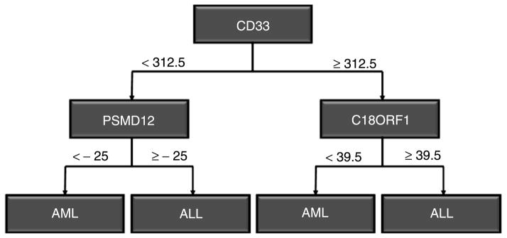
ALL/AML decision tree.

• CD33 < 312.5 AND PSMD12 < −25 OR CD33 > = 312.5 AND C18ORF1 < 39.5 → AML

• CD33 < 312.5 AND PSMD12 > = −25 OR CD33 > = 312.5 AND C18ORF1 > = 39.5 → ALL

A decision tree, however, tends to be a weak distinguisher for cancer subtypes or between normal and cancer samples since it often over-fits the model. In other words, decision tree performs well when training a model that generates a small training error. On the other hand, the performance degrades quickly when applied to the test samples. An ensemble of decision trees can be used to overcome the over-fitting problem. An ensemble model trains a number of classifiers using different subsets of the training data, different features, or different learning methods. Once a set of classifiers (or decision trees) is constructed, the results are integrated through a combination method such as the majority vote algorithm. An ensemble of decision trees was shown to perform better than single decision tree classifiers when applied to cancer microarray data [36–37]. Ensemble learning can improve the performance of a classification model by employing multiple learners (classifiers) and combining their predictions. Two popular ensemble approaches have been used in cancer classification, bagging and random forest. Bagging creates subsets of cancer samples from the training data and samples the training set with replacement. After generating a number of subsets of cancer samples, the subsets are used to learn or to construct a number of decision trees. The predictions of these decision trees are combined through the majority vote algorithm. Random forest is another ensemble approach that combines the bagging approach with the selection from a random subset of features (or genes) rather than from the entire set of features (or genes) [38]. The error in random forests is estimated using the misclassification probability of out-of-bag observations. Specifically, two-thirds of the training set is used to construct a tree while one-third is used as a test set (e.g., out-of-bag) to compute the out-of-bag error estimate. This error estimate represents the number of times the predicted class of a test sample (S_i) is not equal to the true class in all the constructed trees where (S_i) was out-of-bag (or chosen to be in the validation set) averaged across all test samples. Therefore, random forests, through the use of the unbiased out-of-bag error estimate, can avoid over-fitting, and hence cross-validation is not required.

2.3. K-Nearest Neighbor

K-nearest neighbor is a non-parametric classification method that is often used when the underlying distribution (e.g., normal or Gaussian) of the data is unknown. Using this method, cancer samples are transformed to a metric space where distances between samples can be determined. This method is based on a distance function (or similarity measure) such as a Euclidean distance or Pearson correlation between a test sample and its k-nearest training samples. The general idea behind k-nearest neighbor analysis is to classify a test sample based upon the most common (majority) class in its k-nearest training samples.

Figure 4 shows an example of a test sample and its 4-nearest neighbors. Using 4-nearest neighbors, the test sample is assigned to “Class 2” since the majority of its nearest neighbors belong to “Class 2”. Unlike decision trees, k-nearest neighbor does not reveal information about the structure of the data but makes use of the correlation between the expression values of the genes through the distance function employed [12]. Additionally, k-nearest neighbor is sensitive to redundant features because all of the features contribute to the similarity measure between a test sample and its neighbors [39]. Thus, feature selection must be used to eliminate the redundancy among the selected features prior to classification. Also, k-nearest neighbor requires high running time when the training set is large [39]. This is because classification is conducted based on the entire feature set, which can be expensive in computing the distance between a test sample and all the training samples. Finally, the choice of the number of neighbors’ k can greatly affect the performance of the classifier.

Figure 4.

Illustration of 4-nearest neighbors method.

Different measurements for the distance function have been used, including the Euclidean distance, Minkowski’s metric, correlation, etc. K-nearest neighbor using Euclidean as a distance function was shown to achieve high classification accuracy for leukemia and malignant gliomas cancer predictions [40–41]. Similarly, k-nearest neighbor using Euclidean distance and prognostic features (clump thickness, marginal adhesion, single epithelial cell size, etc.) achieved a prediction accuracy of 99.12% for breast cancer survivability [42]. These studies suggest that k-nearest neighbor with a simple distance measure, Euclidean distance, can achieve high classification performance for cancer prediction and prognosis. Although the k-nearest neighbor classification method is simplistic, it has outperformed the more sophisticated approaches such as SVM. For example, two modified versions of k-nearest neighbor, k-discriminant adaptive nearest neighbor and k-local hyper-plane distance nearest neighbor, applied to 5 cancer microarray datasets showed better performance than SVM with either linear (penalty paramater C = 1) or radial basis $\left(\gamma =\frac{1}{\text{number}\text{of}\text{features}},\text{penalty}\text{parameter}C=1\right)$ kernels [43]. In addition to SVM, the reported results show that k-nearest neighbor performs well in practice for cancer prediction, achieves high prediction accuracy, and can outperform other classification methods such as decision tree and Naïve Bayes [44].

2.4. Support Vector Machine

SVM is a supervised learning method widely used in classification and regression analysis. SVM is often used in cancer classification [45–49] and is robust to noise. The robustness to noise was achieved by showing that a regularized SVM is equivalent to a robust optimization problem (e.g., SVM is the solution to robust classification) [50]. SVM builds models by separating the data with either a linear or non-linear decision boundary. SVM finds the hyper-plane that maximizes the margin or separation of the data from the different classes (Figure 5). Specifically, SVM seeks a hyper-plane that best separates the classes by maximizing the distance of the closest training samples to the hyper-plane. For a 2-class (binary) classification problem, samples of one class are located on one side of the hyper-plane while samples of the other class are located on the other side of the hyper-plane.

Figure 5.

Illustration of linear SVM.

Figure 5 shows data points for 2 classes that are linearly separable along with a decision boundary determined by SVM such that the distance from the boundary to the closest training samples is maximized. Thus the 2 classes are considered linearly separable if a hyper-plane w^τx + b = 0 exists where w is a vector, b is a scalar, and the data point (i.e., feature vector containing the gene expression) x is assigned to one of the 2 classes if the following is satisfied:

$$\text{Class}=\{\begin{array}{rr}\hfill -1,& \hfill w^{\tau }x+b\le -1\\ \hfill 1,& \hfill w^{\tau }x+b\ge -1\end{array}$$ (4)

Most datasets are non-linearly separable. In this case, SVM converts the data points into a higher dimensional space through a kernel function and then separates the data with a hyper-plane. Different kernel choices are available (e.g., linear, sigmoid, polynomial, radial basis), each associated with a set of parameters [51], and yielding a decision boundary that can separate cancer subtypes or normal vs. cancer samples. By minimizing a function (e.g., generalization error estimate), a kernel can be selected and its parameters automatically tuned to obtain a set of parameters that yield improved prediction performance [52]. Multi-class SVM is still an active area of study to design an optimal method that can classify more than two classes.

Classification models based on SVMs applied to gene expression data have successfully differentiated among different cancer subtypes as well as between normal and cancer samples [19, 45]. SVMs using three kernels (linear, polynomial, and radial basis) with the parameters degree = 2, penalty parameter C= 1, and $\gamma =\frac{1}{\text{number}\text{of}\text{classes}}$ have been used to classify cancer subtypes based on gene number of classes expression data, with an accuracy as high as 97% [19]. Functional analyses through the Human Genome Index (HGI) identified that 65% of the genes selected by SVM were related to the cancer, lending support to the ability of classification methods in identifying genes involved in cancer-related pathways [19]. Additionally, SVM with a polynomial kernal $\left(\gamma =\frac{1}{\text{number}\text{of}\text{classes}},\text{degree}=3\right)$ achieved a higher classification accuracy than k-nearest neighbor and Naïve Bayes classifiers [46]. Similarly, classification based on SVM with radial basis (γ = 0.02, penalty parameter C = 50) and linear (penalty parameter C = 50) kernels has demonstrated to achieve high classification accuracy on many different (leukemia, colon, prostate, lung, and breast) cancer datasets [47, 48]. Finally, ensemble of SVMs has also been applied to classify cancer samples. A bagged ensemble of linear SVMs (penalty parameter C = 1) was employed to classify malignant tissues and achieved better classification accuracy than single linear SVM classifiers (penalty parameter C = 1) [49]. These studies show that classification using SVM was successfully applied for cancer prediction using different cancer datasets and outperformed other classification approaches (e.g., neural networks, Naïve Bayes, k-nearest neighbor), while retaining genes involved in cancer.

3. APPLICATION OF CLASSIFICATION FOR CANCER TREATMENT AND PROGNOSIS

Classification of cancers has been performed to identify potential biomarkers [14, 19, 53, 54, 55, 56]. The assumption in the application of these methods is that by achieving high prediction accuracy, the selected features of the classification model could be cancer biomarkers and further investigated for their therapeutic potential. In these studies, feature wrappers (iterative feature selection method) based on sequential forward search (SFS) and sequential forward floating search (SFFS) algorithms were employed to identify potential biomarkers where linear discriminant analysis, logistic regression, and SVM (linear and polynomial kernels with degree = 2, γ = 10, penalty parameter C = 1) models were used to measure the accuracy of the selected features in cancer classification [53]. Using SFS and SFFS, it was found that p53-binding protein, Ras suppressor protein, psoriasis-associated protein, and DNA repair gene MSH2, which are related to the development of tumors, were among the features that provided high classification accuracy in classifying BRCA1 mutation-positive tumors. Additionally, it was found that MAPK1, MAPK7, suppression of tumorogenicity, and semia sarcoma viral oncogene homolog, which are involved in tumurogenesis, were among the features that achieved high classification accuracy in classifying BRCA2 mutation-positive tumors. Therefore, the selected features used to build the classification model could be potential biomarkers.

A study of 38 bone marrow samples from acute leukemia patients divided into two groups (AML, ALL) identified 50 genes that were highly correlated with either AML or ALL, based on correlation and a neighborhood analysis method [14]. Supervised learning was used to train a classification model based on these 50 informative genes, which was then applied to a test dataset of 34 leukemia samples, where 29 of the 34 leukemia samples were correctly predicted or classified. It was found that many of the genes used in classifying the AML and ALL samples are known oncogenes (c-MYB, E2A and HOXA9) involved in cancer. Further, one of the selected genes encoded for topoisomerase II, which is a target of the anti-cancer agent etoposide. This supports the use of classification models in identifying possible biomarkers. Thus, using an external feature selection method, a set of informative genes was selected that achieved high classification accuracy with a supervised classification model and could serve as potential biomarkers.

A network-constrained SVM model was applied on 2 breast cancer gene expression datasets to identify cancer biomarkers and to predict clinical outcome of patients [55]. The method integrated gene expression with protein-protein interaction data and identified genes that were highly enriched in pathways related to cancer progression, i.e., cell cycle and cell proliferation. Many of the hub genes identified were enriched in signaling pathways such as TGF-beta, MAPK, and JAK-STAT. Similarly, a combined approach of genetic programming and SVM found many genes involved in tumorgenesis (i.e., ERK/MAPK signaling, Wnt/betacatenin signaling, PI3K/AKT signaling, apoptosis signaling and TGF-beta signaling), supporting classification methods in revealing potential cancer biomarkers [56].

In addition to biomarker discovery, classification methods also have been used to predict patient survivability, cancer recurrence, and prognosis [7, 8, 9, 57, 58, 59, 60]. The prediction of patient survivability or cancer recurrence indicates whether an event (e.g., death or recurrence of a disease) will occur within a specific time. This is achieved by computing the probability of occurrence or predicting the occurrence or non-occurrence of an event. Prediction of cancer recurrence is important in that, for example, the prediction of prostate cancer recurrence helps urologists determine whether to operate on patients with localized prostate cancer [57]. Similarly, the prediction of survival time is an important topic in cancer research where a classification model is learned from training data to predict the time range patients will survive. Such prediction helps to decide whether a patient should receive a treatment or what type of treatment (e.g., chemotherapy) the patient should receive. Because cancer treatments are often associated with side-effects that might lead to death, a model that could predict the survival time of patients without therapy based on certain features could help in the decision-making process of whether to seek treatment or not. Classification models have been successful in predicting survival time. Three different classification methods (artificial neural networks, decision trees, and logistic regression) were applied to cancer statistics data to predict patient survivability [58]. Sixteen variables (grade, stage of cancer, lymph node involvement, extension of disease, etc.) were used to predict the class of a patient (“survive” or “did not survive”). The results were obtained through the use of 10-fold cross-validation, and decision tree was found to outperform other classifiers, achieving a classification accuracy of 93.6%, sensitivity (measures the proportion of true positives correctly identified) of 96.0% and specificity (measures the proportion of true negatives correctly identified) of 90.7%. In another study [59], an artificial neural network classification model, using TNM features, e.g., size of the tumor, distant metastasis, and regional lymph node involvement, was found to outperform the more traditional TNM (T: size of the tumor, N: regional lymph node involvement, M: presence of metastasis) staging system in predicting the 5-year survival rate of breast and colorectal cancer patients using the American College of Surgeons’ Patient Care Evaluation dataset. The artificial neural network model achieved higher prediction accuracy than the TNM staging system (77% vs. 72%). Similar results were obtained when the artificial neural network model was applied to predict the 10-year survival rate of breast cancer patients using the National Cancer Institute’s Surveillance, Epidemiology, and End Results breast carcinoma dataset (73.0% accuracy of artificial neural network vs. 69.2% of TNM). Thus, artificial neural network outperformed the TNM staging system in predicting cancer prognosis. Another approach used artificial neural networks to predict patient survival time based on microarray and clinical data as features [60], and showed that the model achieved high correlation between the observed and the predicted survival times for patients with diffuse large b-cell lymphoma (DLBCL), follicular lymphoma (FL), and ovarian cancer with a correlation coefficient of 0.956281, 0.770620, and 0.86795, respectively.

4. COMPARISON OF METHODS

Most studies evaluate a single classification method, with occasional comparisons performed on more than three methods. To evaluate whether any of the existing classification models discussed above performed better than the others, we applied each of the classification models as well as an ensemble of decision tree classifiers on 5 cancer datasets. Due to the instability of single decision tree classifiers, an ensemble of decision trees (bagging/random forests) was employed. Prior to classification, a two-step feature selection method was applied on 5 cancer datasets to decrease the dimensionality of the feature space and to obtain a set of genes that can best distinguish between different classes (e.g., normal vs. cancer samples). The first step (ReliefF) filters out irrelevant genes that are unable to differentiate between groups, and the second step applies a wrapper heuristic method (e.g., genetic algorithm) to obtain the best set of features for classification. The datasets used were (1) a leukemia dataset containing 72 samples of human acute leukemia, of which 25 are acute myeloid leukemia (AML) and 47 are acute lymphoblastic leukemia (ALL) samples [14], (2) a mixed-lineage leukemia (MLL) dataset, of which 24 are acute lymphoblastic leukemia (ALL), 20 are mixed-lineage leukemia (MLL), and 28 are acute myeloid leukemia (AML) samples [15], (3) a colorectal cancer dataset consisting of 18 cancerous and 18 normal samples [16], (4) a diffuse large B-cell lymphomas (DLBCL) dataset containing 58 samples of diffuse large B-cell lymphoma (DLBCL) and 19 samples of Follicular lymphoma (FL) [17], (5) and a prostate dataset containing 10 normal and 10 prostate cancer samples [18].

4.1. ReliefF

ReliefF, an algorithm that estimates the quality of features (e.g., genes) [61], was employed as a filtering method to decrease the dimensionality of the feature space and to obtain a set of genes that can be used as an input to a second layer wrapper method (e.g., genetic algorithm). ReliefF weighs each gene as to how much it can differentiate among different classes (cancer subtypes or cancer versus normal samples). A gene that differentiates samples belonging to a different class has a higher weight and rank than a gene that differentiates samples belonging to the same class. Additionally, ReliefF assumes that dependency exists between different features (e.g., genes).

Let s_i be a random sample (e.g., normal/cancer sample), H_si be the nearest neighbors belonging to the same class of sample s_i, and M_si be the nearest neighbors belonging to a different class of sample s_i. ReliefF finds a margin such that the distance between s_i and H_si is minimized while the distance between s_i and H_si is maximized:

$$\text{Maximize}[\text{Euclidean}\text{Distance}(s_i,M_{s_i})-\text{Euclidean}\text{Distance}(s_i,H_{s_i})]$$ (5)

Therefore, choosing the k-nearest neighbors of s_i such that they belong to the same class (nearest hits H_si) and the k-nearest neighbors of s_i such that they belong to a different class (nearest misses M_si), the quality estimate of every gene is updated according to the values of s_i, H_si, and M_si.

After applying ReliefF, the genes were ranked according to their weight. Since there is no explicit cut-off, the point of inflection in the plots (Figure 6), which happens to be 10%, was used. Hence, the top 10% of the genes were used as inputs to the genetic algorithm.

Figure 6.

Distribution of Relief scores with respect to features. The dashed line corresponds to the 10% cut-off used. A) Leukemia; B) MLL; C) Colon; D) DLBCL; E) Prostate.

4.2. Genetic Algorithm

The output of ReliefF (top 10% genes) was used as an input to a genetic algorithm to obtain a set of genes that can best differentiate among different classes. We encoded each individual (an individual represents a subset of features) of the genetic algorithm using a binary feature vector (Figure 7), where the size of the vector is equal to the number of genes that are input to the genetic algorithm (e.g., top 10% genes). The values within the binary feature vector determine which features are selected for evaluation (e.g., classification) [62]. A value of 0 in the binary feature vector encodes a feature (e.g., gene) that is not selected for evaluation, while a binary value of 1 encodes a feature (e.g., gene) that is selected for evaluation. Each individual is trained using a subset of features (indices of the feature vector containing a binary value of 1) and evaluated using prediction accuracy.

Figure 7.

Representation of a chromosome (e.g., individual).

The following parameters were used for the genetic algorithm:

• Population size: 100.

• Maximum number of generations: 100.

• Selection method: Tournament selection with size = 2 (two individuals are selected at random and the one with higher fitness value moves to the next generation).

• Elitism rate: 10 individuals.

• Crossover: 2-point crossover with probability 0.6.

• Mutation: Random mutation with probability 0.05.

The initial population is created by randomly assigning binary values (1 or 0) to each individual (e.g., feature vector). The fitness function of every individual is defined as the predictive accuracy of a classification method; each individual is evaluated using the classification methods reviewed (e.g., decision tree, k-nearest neighbor, support vector machine, bagging, and random forest). Leave-one-out cross validation (LOOCV) method, a special case of k-fold cross validation where k is equal to the number of observation in the original sample, was used to avoid over-fitting. In LOOCV, a sample is left out of the training and used to validate the model. Thus, the model is trained on k-1 samples where k corresponds to the number of samples in a dataset. This cross validation method is repeated k times and the average error rate is computed. Since the genetic algorithm is a non-deterministic method, an average of 10 different runs was used to compute the final accuracy.

The two-step feature selection method was run on gene expression data alone and again on the combined gene expression and protein-protein interaction data. The human protein-protein interaction network was obtained from BioGrid (thebiogrid.org). For the integrative approach, the first nearest neighbors of the top 10% of the genes in the protein-protein interaction network as well as the output from ReliefF were used as inputs to the genetic algorithm.

4.3. Tools

LIBSVM [63], a tool that implements SVM, was used to evaluate the genetic algorithm with the following kernels:

• Linear: u′ * v where cost = 1

• Polynomial: (γ * u′ * v)^degree where $\gamma =\frac{1}{\text{number}\text{of}\text{features}}$, degree = 3, cost = 1,

• Radial Basis: e^{(−γ *|u − v|2)} where $\gamma =\frac{1}{\text{number}\text{of}\text{features}}$, cost = 1

• Sigmoid: (γ * u′ * v) where $\gamma =\frac{1}{\text{number}\text{of}\text{features}}$, cost = 1

Matlab’s classregtree function, with Gini index as a splitting criterion, was used to implement the decision trees. Bagging was implemented using Matlab’s TreeBagger function (number of trees = 100) where the number of features to randomly select at each decision split is equal to the number of total features. Similarly, random forest was implemented using Matlab’s TreeBagger function (number of trees = 100) where the number of features to randomly select at each decision split is equal to the square root of the total features. Also, Matlab’s knnclassify function (with Euclidean distance) was used to implement the k-nearest neighbor evaluation method. Additionally, Matlab’s princomp function was used to perform principle component analysis. The two-step feature selection method (ReliefF and genetic algorithm) was implemented in Matlab where the number of nearest neighbors used by ReliefF was set to 5. Finally, it should be noted that classifiers such as SVMs, decision trees, and ensembles (bagging or random forests) also have inherent feature selection methods in their implementation, that select support vectors which are training samples located on the margin of SVMs or deciding upon the splitting criterion for the decision trees and ensembles.

4.4. Results

Figure 8 illustrates the advantage of using a genetic algorithm to select a set of features that can best distinguish among different cancer subtypes or cancer vs. normal samples. Using a genetic algorithm, the performance increases across generations due to the selection of fitter individuals.

Figure 8.

Performance of the genetic algorithm across 100 generations based on gene expression with two evaluation functions: A) Decision Tree, and B) Linear SVM.

The prediction accuracies obtained using 10 different evaluation functions for the two-step feature selection method based on gene expression data are shown in Table 1. Based on the results, linear SVM achieved the highest prediction accuracy of 99.89% with the MLL dataset, slightly outperforming 1-nearest neighbor (99.65%), 5-nearest neighbor (99.47%), polynomial SVM (99.37%), and 3-nearest neighbor (99.26%). Similarly, linear SVM achieved the highest prediction accuracy of 99.4% with the leukemia dataset, followed by polynomial SVM with a prediction accuracy of 99.01%. SVM with the polynomial kernel achieved the highest prediction accuracy of 99.93% with the colon cancer dataset, followed by 1-nearest neighbor, 3-nearest neighbor, 5-nearest neighbor, decision tree, and linear SVM with prediction accuracies of 99.91%, 99.83%, 99.79%, 99.77%, and 99.67%, respectively. Furthermore, 3-nearest neighbor achieved the highest prediction accuracy of 99.69% with the DLBCL dataset, slightly outperforming 1-nearest neighbor (99.67%) and 5-nearest neighbor (99.66%). A decision tree induction approach achieved the highest prediction accuracy of 99.35% on the prostate cancer dataset, largely outperforming the other classifiers.

Table 1.

Prediction accuracies of 10 classifiers for 5 cancer datasets using gene expression

Classifier	Accuracy, %
	MLL	Leukemia	Colon	DLBCL	Prostate
Decision Tree	93.02	96.84	99.77	92.21	99.35
1-nearest neighbor	99.65	98.74	99.91	99.67	89.95
3-nearest neighbor	99.26	97.71	99.83	99.69	89.83
5-nearest neighbor	99.47	97.81	99.79	99.66	94.89
SVM - Linear	99.89	99.40	99.67	99.47	94.84
SVM - Polynomial	99.37	99.01	99.93	99.45	89.90
SVM - Radial Basis	38.89	65.28	23.18	72.69	14.62
SVM - Sigmoid	37.12	70.6	20.41	75.33	15.54
Bagging	94.44	97.22	94.44	90.91	95
Random Forest	98.61	98.61	97.22	93.51	95

Table 2 exhibits the results obtained using 10 different evaluation functions for the two-step feature selection method based on gene expression as well as protein-protein interaction data. The results in Table 2 demonstrate that 1-nearest neighbor, 3-nearest neighbor, 5-nearest neighbor, and linear SVM achieved a maximum prediction accuracy of 100% with the MLL dataset, while random forest achieved the highest prediction accuracy of 100% with the leukemia dataset. For the colon cancer dataset, 7 evaluation functions achieved a maximum prediction accuracy of 100%. The three nearest neighbor methods along with linear SVM achieved the highest prediction accuracy of 100% with the DLBCL dataset. Linear SVM, decision tree, 5-nearest neighbor, and bagging achieved the highest prediction accuracy of 100% with the prostate dataset.

Table 2.

Prediction accuracies of 10 classifiers for 5 cancer datasets using gene expression and protein-protein interaction data

Classifier	Accuracy, %
	MLL	Leukemia	Colon	DLBCL	Prostate
Decision Tree	93.06	97.22	100	92.21	100
1-nearest neighbor	100	99.17	100	100	95
3-nearest neighbor	100	97.78	100	100	99
5-nearest neighbor	100	98.61	100	100	100
SVM - Linear	100	99.72	99.44	100	100
SVM - Polynomial	98.89	98.33	100	99.74	99
SVM - Radial Basis	54.18	71.57	55.95	74.92	25.55
SVM - Sigmoid	52.17	79.22	45.57	83.41	39.22
Bagging	97.22	98.61	100	95.84	100
Random Forest	99.54	100	100	96.1	98

The prediction accuracy obtained using the integrative approach (gene expression and protein-protein interaction) was higher compared to using gene expression alone in 46 out of the 50 cases reported. Such result suggests that combining gene expression data with other genomic information (e.g., protein-protein interaction data) can increase the prediction accuracy. Taking an integrative approach, a perfect classification (accuracy = 100%) was achieved in 20 out of the 50 cases reported. A Wilcoxon rank-sum test was performed to ensure the non-randomness of the difference in the obtained results using gene expression compared to the integrative approach. The two sets of results were found to be significantly different (p = 0.0059). Therefore, these results illustrate that an integrative approach including protein-protein interaction and gene expression data creates more reliable models compared with using gene expression data alone.

To compare the two-step feature selection method with other methods, principle component analysis and ReliefF (alone) based on gene expression were applied to the 5 cancer datasets, and the prediction performances of the aforementioned classifiers were tested. The results in Table 3 show that models based on the two-step feature selection method largely outperformed models based on principle component analysis or ReliefF (alone). Using the two-step feature selection method, higher classification accuracy was achieved in 47 out of the 50 cases reported compared to the principle component analysis approach. Similarly, higher classification accuracy was achieved by the two-step feature selection method than ReliefF (alone) in 46 out of the 50 cases reported. Specifically, the average accuracies achieved by the two-step feature selection method, ReliefF, and principle component analysis were 86.33%, 81.1%, and 76.5%, respectively, illustrating that the two-step feature selection method outperforms the other two (single feature selection) approaches. A Wilcoxon rank-sum test was performed on the two-step feature selection versus PCA, two-step feature selection versus ReliefF, and PCA versus ReliefF, and the results were found to be significant with p-values of 5.24e⁻⁶, 0.0018, and 0.0098, respectively. The results obtained by the two-step feature selection method were further compared with other approaches in the literature. For instance, a multi-test decision tree [34] achieved a prediction accuracy of 85.83%, 85.42%, 91.17%, and 61.76% for the colon cancer, DLBCL, leukemia, and prostate cancer datasets, respectively. By applying the two-step feature selection method with a simple decision tree induction approach as an evaluation function, our method was able to outperform the multi-test decision tree approach by achieving a prediction accuracy of 99.77%, 92.21%, 96.84% and 99.35% on the colon cancer, DLBCL, leukemia, and prostate cancer datasets, respectively. Similarly, the two-step feature selection method used with decision tree, ensemble models (bagging or random forests), k-nearest neighbor (k = 1, 3, or 5), and SVM (linear or polynomial), outperformed the neighborhood analysis method [14] which demonstrated a prediction accuracy of 93.94% for the leukemia dataset.

Table 3.

Prediction accuracies of 10 classifiers for 5 cancer datasets using principle component analysis or ReliefF

Classifier	Accuracy, %
	MLL		Leukemia		Colon		DLBCL		Prostate
	PCA	ReliefF	PCA	ReliefF	PCA	ReliefF	PCA	ReliefF	PCA	ReliefF
Decision Tree	84.72	87.5	72.22	84.72	41.67	94.44	87.01	89.61	45	70
1-nearest neighbor	90.28	95.83	93.06	97.22	97.22	97.22	90.91	94.81	60	80
3-nearest neighbor	93.06	95.83	95.83	95.83	97.22	97.22	89.61	97.4	65	80
5-nearest neighbor	93.06	95.83	94.44	97.22	97.22	97.22	88.31	97.4	75	85
SVM-Linear	97.22	97.22	95.83	97.22	97.22	97.22	96.1	96.1	75	80
SVM-Polynomial	80.56	91.66	80.56	97.22	94.44	97.22	89.61	98.7	70	80
SVM-Radial Basis	25.27	65.27	38.89	38.88	0	0	70.32	75.32	0	0
SVM-Sigmoid	86.11	65.27	67.5	38.88	83.33	0	70.52	75.32	60	0
Bagging	94.44	93.83	83.33	93.06	86.11	94.22	89.21	89.61	80	90
Random Forest	84.72	97.22	72.22	95.83	75	97.22	80.52	92.21	50	90

Building a classification model based on gene expression data, the prostate cancer dataset was the most difficult to classify, with an average accuracy of 77.8920% for all 10 classifiers (Figure 9). Similarly, taking the integrative approach, the prostate dataset was also the most difficult to predict, with an average prediction accuracy of 85.5770%, which is higher than that using gene expression alone. The leukemia and DLBCL datasets were the easiest to classify, with a prediction accuracy of 92.1220% and 92.2590%, respectively, using gene expression, and 94.0230% and 94.2220%, respectively, using an integrative approach.

Figure 9.

Average accuracy of the 5 cancer datasets for all 10 classifiers using gene expression and the integrative approach.

As shown in Figure 10, the highest average accuracy of a classifier for all 5 cancer datasets based on gene expression was achieved by linear SVM (98.6540%), followed by 5-nearest neighbor (98.3240%). Similarly, linear SVM (99.8320%) achieved the highest performance using the integrative approach, followed by 5-nearest neighbor (99.7220%). On the other hand, the worst performing prediction method was the radial basis SVM, with a prediction accuracy of 42.9320% for the gene expression approach and 56.4340% for the integrative approach.

Figure 10.

Average accuracy of the 10 classifiers for the 5 cancer datasets using gene expression and the integrative approach.

5. DISCUSSION

Genetic algorithms are computationally expensive and infeasible when the feature set is large. Therefore, applying a filter method that reduces the dimensionality of the feature space and removes unimportant/irrelevant genes is essential. ReliefF is a feature estimator method that accounts for dependencies among features, weighs each gene based on its ability to differentiate between groups to obtain a candidate gene set. Applying ReliefF reduces the computational complexity of the genetic algorithm. On other hand, applying ReliefF alone does not perform well because of the small sample sizes of most microarray datasets. A genetic algorithm could mitigate this problem by conducting an optimized search on the candidate gene set obtained by ReliefF to select the best subset of features. Therefore, the integration of ReliefF and genetic algorithms leads to an effective two-step feature selection method that can best differentiate among classes.

The choice of the evaluation function (e.g., classifier) is essential for a feature selection method to achieve high prediction accuracy. For the two-step feature selection method presented, linear and polynomial SVM as well as k-nearest neighbors with k = 1, 3, and 5 are shown to achieve higher prediction accuracies than radial basis and sigmoid SVM. This suggests that using simpler SVM kernels could be sufficient for most cases. The two-step feature selection method achieved a relatively high performance in 8 out of the 10 classifiers tested based on gene expression alone or an integrative approach based on gene expression and protein-protein interaction data, thereby suggesting the method is robust. The simplistic approach of k-nearest neighbor achieved high performance across all 5 datasets, because decisions on test samples are made based on the entire training set, this is in contrast to SVMs (e.g., Sigmoid and Radial SVMs) which use a subset of the data (i.e., support vectors) to form the margin (separation). Even though decision tree classifiers use the whole training set, they are considered unstable learning methods because small changes in the selected features or the training data could cause a drastic change in the decision tree structure. In the analysis, decision trees achieved a maximum classification performance with the colon and prostate datasets, but were outperformed with the leukemia and DLBCL datasets that used the other classification methods. This high performance achieved by decision trees is largely due to the genetic algorithm which conducts an optimized search for a set of features (e.g., genes) to be used as an input for splitting a decision tree. Ensemble approaches (e.g., bagging and random forest) applied to decision trees were significantly outperformed by most of the other classifiers based on gene expression. However, using an integrative approach, ensemble models achieved a relatively high classification performance across all 5 cancer datasets.

Based on the results of Table 1, there is no classification method (individual or ensemble) that universally outperforms all other classifiers; however, on average, k-nearest neighbor (k = 1, 3, or 5) and linear SVM achieved the highest prediction accuracy across different cancer datasets. However, as a challenge with cancer classification, a classification method can be designed to outperform all others for a specific dataset, but can be easily outperformed when tested on a different dataset. Furthermore, the small number of samples and the large number of features (genes) compound the difficulties in designing a model for cancer classification that consistently achieves high prediction accuracy with small training time across different datasets.

Studies have suggested that the integration of gene expression and other biologically relevant information can create more reliable models. For example, an algorithm that integrates gene expression data with network information (i.e., protein-protein interaction data) achieved high classification accuracy and improvement in the biological interpretability of the results [64]. Similarly, a genetic algorithm was employed to identify subnetwork markers for predicting breast cancer metastasis [65] where high classification accuracy was achieved using any of the 6 classification methods (logistic regression, SVM, decision tree, Adaboost, random forest, and Logiboost), thereby creating a robust model that is more consistent and accurate than models based on gene expression data. An integrative approach [66] that combined protein-protein interaction and gene expression data identified biomarkers for breast cancer metastasis, and found genes highly enriched in cell cycle, apoptosis, DNA repair, Jak-STAT, MAPK, ErbB, Wnt, and p53 signaling pathways where the overlap of the identified genes across different microarray datasets using the integrative approach was significantly higher than models based on gene expression data alone.

Similarly, the two-step feature selection method achieved improved prediction accuracy based on an integrative approach compared to using gene expression alone. Additionally, the two-step feature selection approach achieved high classification accuracy across a diverse set of evaluation functions (e.g., SVM, k-nearest neighbors, decision trees, and ensemble approaches), suggesting that the approach is not sensitive to the choice of classifier. The two-step feature selection method retained known biomarkers across all 5 cancer datasets tested in the present study. Specifically, it retained genes that are known to be related to these cancers. The identified genes were repeatedly selected by the genetic algorithm across many generations due to their ability to differentiate different cancer subtypes or cancerous versus normal samples. The top four repeatedly selected genes by the genetic algorithm in the colon dataset were the following: MSH2, a gene known to be associated with hereditary nonpolyposis colorectal cancer [67]; CLU, a gene associated with cancer promotion, metastasis and pro-survival processes [68]; TAGLN, a diagnostic marker of colon cancer; and IGF2R, a mutated gene identified in colon cancer. Using the prostate cancer dataset, the top gene repeatedly selected by the genetic algorithm was MDM2, an oncoprotein which is a cellular inhibitor of p53 and an inhibitor of the activation of genes involved in cell cycle arrest and apoptosis [69]. Furthermore, using the DLBCL dataset, RhoH and MUM1 (prognostic factors for DLBCL), BCL6 (an oncogene involved in chromosomal translocation), and ICAM1 (a cell surface receptor involved in lymphoid trafficking and extravasation [70]) were the top four genes repeatedly selected by the genetic algorithm. TCF3 (a gene involved in the Wnt signaling pathway), FLT3 (a proto-oncogene), and ANPEP were the top three genes in the leukemia dataset. In addition to retaining known genes involved in the different cancers, the two-step feature selection method was also able to identify potential novel genes among the top ranked list of genes.

6. CONCLUSION

Cancer classification has been useful in predicting cancer survivability and recurrence. Thus far, cancer classification has identified potential biomarkers involved in cancer-related pathways. Biomarker identification could improve if more and diverse data types are integrated into the classification models, as with the integration of protein-protein interaction data. Nevertheless, a challenge remains in that there is no classification approach that can perfectly classify all types of cancers. However, the integration of gene expression data with network and other genomic data could improve upon the classification models based on gene expression data alone to achieve better predictions of cancer and identification of cancer biomarkers that could be potential therapeutic targets.

APPENDIX

A Naïve Bayes is a probabilistic classifier that estimates the probability of attributes (or features), under the assumption that the features are conditionally independent given a class y, from the training data:

$$P\left(x_1,x_2,x_3,x_n\mid y\right)=P(x_1\mid y)P(x_2\mid y)P(x_n\mid y)$$ (A1)

The classification process using a naïve Bayes approach starts by estimating P(x₁|y)…P(x_n|y) as well as P(y) using the training data. The second step classifies a test sample by choosing the class that maximizes the following probability:

$$\text{Class}=\underset{y}{argmax}P\left(x_1\mid y\right)P\left(x_2\mid y\right)P(x_n\mid y)P(y)$$ (A2)

References

- 1.Harrington CA, Rosenow C, Retief J. Monitoring gene expression using DNA microarrays. Curr Opin Microbiol. 2000;3(3):285–91. doi: 10.1016/s1369-5274(00)00091-6. [DOI] [PubMed] [Google Scholar]
- 2.Schena M, Shalon D, Davis RW, Brown PO. Quantitative monitoring of gene expression patterns with a complementary DNA microarray. Science. 1995;270:467–70. doi: 10.1126/science.270.5235.467. [DOI] [PubMed] [Google Scholar]
- 3.Liu Q, Sung AH, Chen Z, Liu J, Chen L, Qiao M, Wang Z, Huang X, Deng Y. Gene selection and classification for cancer microarray data based on machine learning and similarity measures. BMC Genomics. 2011;12 (Suppl 5):S1. doi: 10.1186/1471-2164-12-S5-S1. [DOI] [PMC free article] [PubMed] [Google Scholar]
- 4.Liu JJ, Cai WS, Shao XG. Cancer classification based on microarray gene expression data using a principal component accumulation method. SCIENCE CHINA Chemistry. 2011;54(5):802–11. [Google Scholar]
- 5.Dudoit S, Fridlyand J, Speed TP. Comparison of discrimination methods for the classification of tumors using gene expression data. J Am Stat Assoc. 2002;97:77–87. [Google Scholar]
- 6.Xiong M, Jin L, Li W, Boerwinkle E. Computational Methods for Gene Expression-Based Tumor Classification. BioTechniques. 2000;29(6):1264–1270. doi: 10.2144/00296bc02. [DOI] [PubMed] [Google Scholar]
- 7.Vanneschi L, Farinaccio A, Mauri G, Antoniotti M, Provero P, Giacobini M. A Comparison of Machine Learning Techniques for Survival Prediction in Breast Cancer. BioData Min. 2011;4:1–12. doi: 10.1186/1756-0381-4-12. [DOI] [PMC free article] [PubMed] [Google Scholar]
- 8.Bard E, Hu W. Identification of a 12-Gene Signature for Lung Cancer Prognosis through Machine Learning. Journal of Cancer Therapy. 2011;2(2):148–156. [Google Scholar]
- 9.Gupta S, Kumar D, Sharma A. Data Mining Classification Techniques Applied for Breast Cancer Diagnosis and Prognosis. Indian Journal of Computer Science and Engineering. 2011;2(2):188–195. [Google Scholar]
- 10.George GVS, Raj VC. Review on Feature Selection Techniques and the Impact of SVM for Cancer Classification using Gene Expression Profile. International Journal of Computer Science & Engineering Survey. 2011;2(3):1–12. [Google Scholar]
- 11.Asyali MH, Colak D, Demirkaya O, Inan MS. Gene expression profile classification: a review. Curr Bioinformatics. 2006;1:55–73. [Google Scholar]
- 12.Lu Y, Han J. Cancer classification using gene expression data. Inform Syst. 2003;28(4):243–268. [Google Scholar]
- 13.Cruz JA, Wishart DS. Applications of Machine Learning in Cancer Prediction and Prognosis. Cancer Inform. 2006;2:59–77. [PMC free article] [PubMed] [Google Scholar]
- 14.Golub TR, Slonim DK, Tamayo P, Huard C, Gaasenbeek M, Mesirov JP, Coller H, Loh ML, Downing JR, Caligiuri MA, Bloomfield CD, Lander ES. Molecular classification of cancer: class discovery and class prediction by gene expression monitoring. Science. 1999;286:531–37. doi: 10.1126/science.286.5439.531. [DOI] [PubMed] [Google Scholar]
- 15.Armstrong SA, Staunton JE, Silverman LB, Pieters R, den Boer ML, Minden MD, Sallan SE, Lander ES, Golub TR, Korsmeyer SJ. MLL translocations specify a distinct gene expression profile that distinguishes a unique leukemia. Nat Genet. 2002;30(1):41–7. doi: 10.1038/ng765. [DOI] [PubMed] [Google Scholar]
- 16.Notterman DA, Alon U, Sierk AJ, Levine AJ. Transcriptional Gene Expression Profiles of Colorectal Adenoma, Adenocarcinoma, and Normal Tissue Examined by Oligonucleotide Arrays. Cancer Res. 2001;61:3124–30. [PubMed] [Google Scholar]
- 17.Shipp MA, Ross KN, Tamayo P, Weng AP, Kutok JL, Aguiar RC, Gaasenbeek M, Angelo M, Reich M, Pinkus GS, Ray TS, Koval MA, Last KW, Norton A, Lister TA, Mesirov J, Neuberg DS, Lander ES, Aster JC, Golub TR. Diffuse large B–cell lymphoma outcome prediction by gene-expression profiling and supervised machine learning. Nat Med. 2002;8(1):68–74. doi: 10.1038/nm0102-68. [DOI] [PubMed] [Google Scholar]
- 18.Singh D, Febbo PG, Ross K, Jackson DG, Manola J, Ladd C, Tamayo P, Renshaw AA, D’Amico AV, Richie JP, Lander ES, Loda M, Kantoff PW, Golub TR, Sellers WR. Gene expression correlates of clinical prostate cancer behavior. Cancer Cell. 2002;1(2):203–9. doi: 10.1016/s1535-6108(02)00030-2. [DOI] [PubMed] [Google Scholar]
- 19.Shieh GS, Bai CH, Lee C. Identify Breast Cancer Subtypes by Gene Expression Profiles. Journal of Data Science. 2004;2:165–175. [Google Scholar]
- 20.Chen AH, Tsau YW, Wang YC. A novel multi-task support vector sample learning technique to predict classification of cancer. New Trends in Information Science and Service Science (NISS) 2010:196–200. [Google Scholar]
- 21.Pittman J, Huang E, Dressman H, Horng CF, Cheng SH, Tsou MH, Chen CM, Bild A, Iversen ES, Huang AT, Nevins JR, West M. Integrated modeling of clinical and gene expression information for personalized prediction of disease outcomes. Proc Natl Acad Sci USA. 2004;101(22):8431–8436. doi: 10.1073/pnas.0401736101. [DOI] [PMC free article] [PubMed] [Google Scholar]
- 22.Saeys Y, Inza I, Larranaga P. A review of feature selection techniques in bioinformatics. Bioinformatics. 2007;23(19):2507–2517. doi: 10.1093/bioinformatics/btm344. [DOI] [PubMed] [Google Scholar]
- 23.Jafari P, Azuaje F. An assessment of recently published gene expression data analyses: reporting experimental design and statistical factors. BMC Med Inform Decis Mak. 2006;6:27. doi: 10.1186/1472-6947-6-27. [DOI] [PMC free article] [PubMed] [Google Scholar]
- 24.Tan F, Fu X, Zhang Y, Bourgeois AG. Improving feature subset selection using a genetic algorithm for microarray gene expression data. Proc IEEE Congr Evolut Comput. 2006:2529–2534. [Google Scholar]
- 25.Tan F, Fu X, Zhang Y, Bourgeois AG. A genetic algorithm–based method for feature subset selection. Soft Comput. 2007;12(2):111–120. [Google Scholar]
- 26.Sardana M, Agrawal RK. A Comparative Study of Clustering Methods for Relevant Gene Selection in Microarray Data. In: Wyld DC, Zizka J, Nagamalai D, editors. Advances in Computer Science, Engineering & Applications. Vol. 166. Springer; Berlin Heidelberg: 2012. pp. 789–797. [Google Scholar]
- 27.Getz G, Levine E, Domany E. Coupled Two-Way Clustering Analysis of Gene Microarray Data. Proc Natural Academy of Sciences US. 2000;97(22):12079–84. doi: 10.1073/pnas.210134797. [DOI] [PMC free article] [PubMed] [Google Scholar]
- 28.Au W, Chan KCC, Wong AKC, Wang Y. Attribute clustering for grouping, selection, and classification of gene expression data. IEEE/ACM Transactions on Computational Biology and Bioinformatics. 2005;2(2):83–101. doi: 10.1109/TCBB.2005.17. [DOI] [PubMed] [Google Scholar]
- 29.Nakkeeran R, Victoire TAA. Hybrid Approach of Data Mining Techniques, PCA, EDM and SVM for Cancer Gene Feature Selection and Classification. European Journal of Scientific Research. 2012;79(4):638–652. [Google Scholar]
- 30.Li X, Peng S, Chen J, Lü B, Zhang H, Lai M. SVM–T-RFE: A novel gene selection algorithm for identifying metastasis-related genes in colorectal cancer using gene expression profiles. Biochem Biophys Res Commun. 2012;419(2):148–153. doi: 10.1016/j.bbrc.2012.01.087. [DOI] [PubMed] [Google Scholar]
- 31.Singh VP, Arvind SG, Mahapatra AG. Hybrid Correlation based Gene Selection for Accurate Cancer Classification of Gene Expression Data. International Journal of Computer Applications. 2012;43(14):13–18. [Google Scholar]
- 32.Netto OP, Nozawa SR, Mitrowsky RAR, Mecedo AA, Baranauskas JA. Applying Decision Trees to Gene Expression Data from DNA Microarray: A Leukemia Case Study. XXX Proc. Of Workshop de Informatica Medica; Belo Horizonte, MG. 2010. pp. 1489–1498. [Google Scholar]
- 33.Zhang H, Yu CY, Singer B, Xiong M. Recursive partitioning for tumor classification with gene expression microarray data. Proc Natl Acad Sci USA. 2001;98(12):6730–5. doi: 10.1073/pnas.111153698. [DOI] [PMC free article] [PubMed] [Google Scholar]
- 34.Czajkowski M, Grzes M, Kretowski M. Multi-Test decision trees for gene expression data analysis. In: Bouvry P, Kłopotek MA, Leprévost F, Marciniak M, Mykowiecka A, editors. Proceedings of the 2011 international conference on Security and Intelligent Information Systems. Vol. 7053. Springer; Berlin Heidelberg: 2012. pp. 154–167. [Google Scholar]
- 35.Dimitoglou G, Adams JA, Jim CM. Comparison of the C4. 5 and a Naive Bayes Classifier for the Prediction of Lung Cancer Survivability. CoRR. 2012;4(8):1–9. [Google Scholar]
- 36.Tan AC, Gilbert D. Ensemble machine learning on gene expression data for cancer classification. Applied Bioinformatics. 2003;2(3):75–83. [PubMed] [Google Scholar]
- 37.Snousy MBA, El-Deeb HM, Badran K, Khlil IAA. Suite of decision tree-based classification algorithms on cancer gene expression data. Egyptian Informatics Journal. 2011;12(2):73–82. [Google Scholar]
- 38.Chen X, Ishwaran H. Random forests for genomic data analysis. Genomics. 2012;99(6):323–9. doi: 10.1016/j.ygeno.2012.04.003. [DOI] [PMC free article] [PubMed] [Google Scholar]
- 39.Cunningham P, Delany SJ. Technical Report UCD-CSI. School of Computer Science and Informatics, University College Dublin; Ireland: 2007. k-Nearest Neighbor Classifiers; p. 4. [Google Scholar]
- 40.Nutt CL, Mani DR, Betensky RA, Tamayo P, Cairncross JG, Ladd C, Pohl U, Hartmann C, McLaughlin ME, Batchelor TT, Black PM, Deimling AV, Pomeroy SL, Golub TR, Louis DN. Gene expression-based classification of malignant gliomas correlates better with survival than histological classification. Cancer Res. 2003;63(7):1602–1607. [PubMed] [Google Scholar]
- 41.Shahbaz M, Faruq S, Shaheen M, Masood SA. Cancer Diagnosis Using Data Mining Technology. Life Science Journal. 2012;9(1):308–313. [Google Scholar]
- 42.Sarkar M, Leong TY. Application of K-nearest neighbors algorithm on breast cancer diagnosis problem. Proc AMIA Symp. 2000:759–763. [PMC free article] [PubMed] [Google Scholar]
- 43.Niijima S, Kuhara S. Effective nearest neighbor methods for multiclass cancer classification using microarray data. Proceedings of the 16th International Conference on Genome Informatics. 2005:51. [Google Scholar]
- 44.Li T, Zhang C, Ogihara M. A comparative study of feature selection and multiclass classification methods for tissue classification based on gene expression. Bioinformatics. 2004;20(15):2429–37. doi: 10.1093/bioinformatics/bth267. [DOI] [PubMed] [Google Scholar]
- 45.Baboo SS, Sasikala S. Multicategory Classification Using Support Vector Machine for Microarray Gene Expression Cancer Diagnosis. Global Journal of Computer Science and Technology. 2010;10(15):38–44. [Google Scholar]
- 46.Wahed ESA, Emam IA, Badr A. Feature Selection for Cancer Classification: An SVM based Approach. International Journal of Computer Applications. 2012;46(8):20–26. [Google Scholar]
- 47.Gao S, Addam O, Qabaja A, ElSheikh A, Zarour O, Nagi M, Triant F, Almansoori W, Ozyer OST, Jia Z, Rokne J, Alhajja R. Robust Integrated Framework for Effective Feature Selection and Sample Classification and Its Application to Gene Expression Data Analysis. Computational Intelligence in Bioinformatics and Computational Biology (CIBCB) 2012:112–119. [Google Scholar]
- 48.Nikumbh S, Ghosh S, Jayaraman V. Biogeography-Based Informative Gene Selection and Cancer Classification Using SVM and Random Forests. IEEE World Congress on Computational Intelligence. 2012:10–15. [Google Scholar]
- 49.Valentini G, Muselli M, Ruffino F. Cancer recognition with bagged ensembles of support vector machines. Neurocomputing. 2004;56:461–466. [Google Scholar]
- 50.Xu H, Caramanis C, Mannor S. Robustness and regularization of support vector machines. J Mach Learn Res. 2009;10:1485–1510. [Google Scholar]
- 51.Suykens J, van Gestel T, De Brabanter J, De Moor B, Vandewalle J. Least Square Support Vector Machines. World Scientific; Singapore: 2002. [Google Scholar]
- 52.Chapelle O, Vapnik V, Bousquet O, Mukherjee S. Choosing Multiple Parameters for Support Vector Machines. Machine Learning. 2002;46:131–159. [Google Scholar]
- 53.Xiong M, Fang Z, Zhao J. Biomarker Identification by Feature Wrappers. Genome Research. 2001;11:1878–1887. doi: 10.1101/gr.190001. [DOI] [PMC free article] [PubMed] [Google Scholar]
- 54.Abeel T, Helleputte T, Van de Peer Y, Dupont P, Saeys Y. Robust biomarker identification for cancer diagnosis with ensemble feature selection methods. Bioinformatics. 2010;26(3):392–8. doi: 10.1093/bioinformatics/btp630. [DOI] [PubMed] [Google Scholar]
- 55.Chen L, Xuan J, Riggins RB, Clarke R, Wang Y. Identifying cancer biomarkers by network-constrained support vector machines. BMC Syst Biol. 2011;5:161. doi: 10.1186/1752-0509-5-161. [DOI] [PMC free article] [PubMed] [Google Scholar]
- 56.Liu JJ, Cutler G, Li W, Pan Z, Peng S, Hoey T, Chen L, Ling XB. Multiclass cancer classification and biomarker discovery using GA-based algorithms. Bioinformatics. 2005;21(11):2691–97. doi: 10.1093/bioinformatics/bti419. [DOI] [PubMed] [Google Scholar]
- 57.Zupan B, Demsar J, Kattan MW, Beck JR, Bratko I. Machine learning for survival analysis: A case study on recurrence of prostate cancer. Artificial Intelligence in Medicine. 2000;20(1):59–75. doi: 10.1016/s0933-3657(00)00053-1. [DOI] [PubMed] [Google Scholar]
- 58.Delen D, Walker G, Kadam A. Predicting breast cancer survivability: a comparison of three data mining methods. Artif Intell Med. 2005;34(2):113–27. doi: 10.1016/j.artmed.2004.07.002. [DOI] [PubMed] [Google Scholar]
- 59.Burke HB, Goodman PH, Rosen DB, Henson DE, Weinstein JN, Harrell FE, Marks JR, Winchester DP, Bostwick DG. Artificial neural networks improve the accuracy of cancer survival prediction. Cancer. 1997;79(4):857–862. doi: 10.1002/(sici)1097-0142(19970215)79:4<857::aid-cncr24>3.0.co;2-y. [DOI] [PubMed] [Google Scholar]
- 60.Chen YC, Yang WW, Chiu HW. Artificial neural network prediction for cancer survival time by gene expression data. Bioinformatics and Biomedical Engineering, 3rd International Conference. 2009:1–4. [Google Scholar]
- 61.Robnik-Šikonja M, Kononenko I. Theoretical and Empirical Analysis of ReliefF and RReliefF. Mach Learn. 2003;53:23–69. [Google Scholar]
- 62.Zhang P, Verma B, Kumar K. Neural Vs Statistical Classifier in Conjunction with Genetic Algorithm Based Feature Selection. J Patt Recog Lett. 2005;26:909–919. [Google Scholar]
- 63.Chang CC, Lin CJ. LIBSVM : a library for support vector machines. ACM Transactions on Intelligent Systems and Technology. 2011;2(3):1–27. Software available at http://www.csie.ntu.edu.tw/~cjlin/libsvm. [Google Scholar]
- 64.Yousef M, Ketany M, Manevitz L, Showe LC, Showe MK. Classification and biomarker identification using gene network modules and support vector machines. BMC Bioinformatics. 2009;10:337. doi: 10.1186/1471-2105-10-337. [DOI] [PMC free article] [PubMed] [Google Scholar]
- 65.Wu J, Gan M, Jiang R. A Genetic Algorithm for Optimizing Subnetwork Markers for the Study of Breast Cancer Metastasis. Natural Computation (ICNC) 2011;3:1578–82. [Google Scholar]
- 66.Jahid MJ, Ruan J. Identification of biomarkers in breast cancer metastasis by integrating protein-protein interaction network and gene expression data. Genomic Signal Processing and Statistics (GENSIPS) 2011:60–63. [Google Scholar]
- 67.Fishel R, Lescoe MK, Rao MR, Copeland NG, Jenkins NA, Gather J, Kane M, Kolodner R. The human mutator gene homolog MSH2 and its association with hereditary nonpolyposis colon cancer. Cell. 1993;75(5):1027–38. doi: 10.1016/0092-8674(93)90546-3. [DOI] [PubMed] [Google Scholar]
- 68.Mazzarelli P, Pucci S, Spagnoli LG. CLU and colon cancer. The dual face of CLU: from normal to malignant phenotype. Adv Cancer Res. 2009;105:45–61. doi: 10.1016/S0065-230X(09)05003-9. [DOI] [PubMed] [Google Scholar]
- 69.Leite KR, Franco MF, Srougi M, Nesrallah LJ, Nesrallah A, Bevilacqua RG, Darini E, Carvalho CM, Meirelles MI, Santana I, Camara-Lopes LH. Abnormal expression of MDM2 in prostate carcinoma. Mod Pathol. 2001;14(5):428–36. doi: 10.1038/modpathol.3880330. [DOI] [PubMed] [Google Scholar]
- 70.Wawryk SO, Novotny JR, Wicks IP, Wilkinson D, Maher D, Salvaris E, Welch K, Fecondo J, Boyd AW. The role of LFA-1/ICAM-1 interaction in human leukocyte homing and adhesion. Immunol Rev. 1989;108:135–161. doi: 10.1111/j.1600-065x.1989.tb00016.x. [DOI] [PubMed] [Google Scholar]