

Significance
Spectral algorithms are widely applied to data clustering problems, including finding communities or partitions in graphs and networks. We propose a way of encoding sparse data using a “nonbacktracking” matrix, and show that the corresponding spectral algorithm performs optimally for some popular generative models, including the stochastic block model. This is in contrast with classical spectral algorithms, based on the adjacency matrix, random walk matrix, and graph Laplacian, which perform poorly in the sparse case, failing significantly above a recently discovered phase transition for the detectability of communities. Further support for the method is provided by experiments on real networks as well as by theoretical arguments and analogies from probability theory, statistical physics, and the theory of random matrices.
Abstract
Spectral algorithms are classic approaches to clustering and community detection in networks. However, for sparse networks the standard versions of these algorithms are suboptimal, in some cases completely failing to detect communities even when other algorithms such as belief propagation can do so. Here, we present a class of spectral algorithms based on a nonbacktracking walk on the directed edges of the graph. The spectrum of this operator is much better-behaved than that of the adjacency matrix or other commonly used matrices, maintaining a strong separation between the bulk eigenvalues and the eigenvalues relevant to community structure even in the sparse case. We show that our algorithm is optimal for graphs generated by the stochastic block model, detecting communities all of the way down to the theoretical limit. We also show the spectrum of the nonbacktracking operator for some real-world networks, illustrating its advantages over traditional spectral clustering.
Detecting communities or modules is a central task in the study of social, biological, and technological networks. Two of the most popular approaches are statistical inference, where we fix a generative model such as the stochastic block model to the network (1, 2); and spectral methods, where we classify vertices according to the eigenvectors of a matrix associated with the network such as its adjacency matrix or Laplacian (3).
Both statistical inference and spectral methods have been shown to work well in networks that are sufficiently dense, or when the graph is regular (4–8). However, for sparse networks with widely varying degrees, the community detection problem is harder. Indeed, it was recently shown (9–11) that there is a phase transition below which communities present in the underlying block model are impossible for any algorithm to detect. Whereas standard spectral algorithms succeed down to this transition when the network is sufficiently dense, with an average degree growing as a function of network size (8), in the case where the average degree is constant these methods fail significantly above the transition (12). Thus, there is a large regime in which statistical inference succeeds in detecting communities, but where current spectral algorithms fail.
It was conjectured in ref. 11 that this gap is artificial and that there exists a spectral algorithm that succeeds all of the way to the detectability transition even in the sparse case. Here, we propose an algorithm based on a linear operator considerably different from the adjacency matrix or its variants: namely, a matrix that represents a walk on the directed edges of the network, with backtracking prohibited. We give strong evidence that this algorithm indeed closes the gap.
The fact that this operator has better spectral properties than, for instance, the standard random walk operator, has been used in the past in the context of random matrices and random graphs (13–15). In the theory of zeta functions of graphs, it is known as the edge adjacency operator, or the Hashimoto matrix (16). It has been used to show fast mixing for the nonbacktracking random walk (17), and arises in connection to belief propagation (18, 19), in particular to rigorously analyze the behavior of belief propagation for clustering problems on regular graphs (5). It has also been used as a feature vector to classify graphs (20). However, we are not aware of work using this operator for clustering or community detection.
We show that the resulting spectral algorithms are optimal for networks generated by the stochastic block model, finding communities all of the way down to the detectability transition. That is, at any point above this transition, there is a gap between the eigenvalues related to the community structure and the bulk distribution of eigenvalues coming from the random graph structure, allowing us to find a labeling correlated with the true communities. In addition to our analytic results on stochastic block models, we also illustrate the advantages of the nonbacktracking operator over existing approaches for some real networks.
Spectral Clustering and Sparse Networks
To study the effectiveness of spectral algorithms in a specific ensemble of graphs, suppose that a graph G is generated by the stochastic block model (1). There are q groups of vertices, and each vertex v has a group label  . Edges are generated independently according to a
  matrix p of probabilities, with
  . In the sparse case, we have
 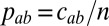 , where the affinity matrix
  stays constant in the limit
  .
.
For simplicity we first discuss the commonly studied case where c has two distinct entries,  if
if  and
and  if
if  . We take
  with two groups of equal size, and assume that the network is assortative, i.e.,
  . The section More than Two Groups and General Degree Distributions below discusses our results in more general cases.
The group labels are hidden from us, and our goal is to infer them from the graph. Let  denote the average degree. The detectability threshold (9–11) states that in the limit
  , unless
the randomness in the graph washes out the block structure to the extent that no algorithm can label the vertices better than chance. Moreover, ref. 11 proved that below this threshold it is impossible to identify the parameters  and
and  , whereas above the threshold the parameters
  and
and  are easily identifiable.
The adjacency matrix is defined as the  matrix
  if
if  and 0 otherwise. A typical spectral algorithm assigns each vertex a k-dimensional vector according to its entries in the first k eigenvectors of A for some k, and clusters these vectors according to a heuristic such as the k-means algorithm (often after normalizing or weighting them in some way). In the case
  , we can simply label the vertices according to the sign of the second eigenvector.
As shown in ref. 8, spectral algorithms succeed all of the way down to the threshold 1 if the graph is sufficiently dense. In that case, A’s spectrum has a discrete part and a continuous part in the limit  . Its first eigenvector essentially sorts vertices according to their degree, whereas the second eigenvector is correlated with the communities. The second eigenvalue is given by
 |
The question is when this eigenvalue gets lost in the continuous bulk of eigenvalues coming from the randomness in the graph. This part of the spectrum, like that of a sufficiently dense Erdős–Rényi random graph, is asymptotically distributed according to Wigner’s semicircle law (21),  . Thus, the bulk of the spectrum lies in the interval
  . If
. If  , which is equivalent to 1, the spectral algorithm can find the corresponding eigenvector, and it is correlated with the true community structure.
However, in the sparse case where c is constant while n is large, this picture breaks down due to a number of reasons. Most importantly, the leading eigenvalues of A are dictated by the vertices of highest degree, and the corresponding eigenvectors are localized around these vertices (22). As n grows, these eigenvalues exceed  , swamping the community-correlated eigenvector, if any, with the bulk of uninformative eigenvectors. As a result, spectral algorithms based on A fail a significant distance from the threshold given by 1. Moreover, this gap grows as n increases: for instance, the largest eigenvalue grows as the square root of the largest degree, which is roughly proportional to
  for Erdős–Rényi graphs. To illustrate this problem, the spectrum of A for a large graph generated by the block model is depicted in Fig. 1.
Fig. 1.

Spectrum of the adjacency matrix of a sparse network generated by the block model (excluding the zero eigenvalues). Here,  ,
,  , and
, and  , and we average over 20 realizations. Even though the eigenvalue
  given by Eq. 2 satisfies the threshold condition 1 and lies outside the semicircle of radius
  , deviations from the semicircle law cause it to get lost in the bulk, and the eigenvector of the second largest eigenvalue is uncorrelated with the community structure. As a result, spectral algorithms based on A are unable to identify the communities in this case.
Other popular operators for spectral clustering include the Laplacian  , where
  is the diagonal matrix of vertex degrees, the symmetrically normalized Laplacian
  , the stochastic random walk matrix
  , and the modularity matrix
  . However, like A, these are prey to localized eigenvectors in the sparse case.
Another simple heuristic is to simply remove the high-degree vertices (e.g., ref. 6), but this throws away a significant amount of information; in the sparse case it can even destroy the giant component, causing the graph to fall apart into disconnected pieces (23). Finally, one can also regularize the adjacency matrix by adding a small constant term (24); however, this introduces a tunable parameter, and we have not explored this here.
Nonbacktracking Operator
The main contribution of this paper is to show how to redeem the performance of spectral algorithms in sparse networks by using a different linear operator. The nonbacktracking matrix B is a  matrix, defined on the directed edges of the graph. Specifically,
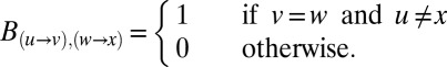 |
Using B rather than A addresses the problem described above. The spectrum of B is not sensitive to high-degree vertices, because a walk starting at v cannot turn around and return to it immediately. Other convenient properties of B are that any tree dangling off the graph, or disconnected from it, simply contributes zero eigenvalues to the spectrum, because a nonbacktracking walk is forced to a leaf of the tree where it has nowhere to go. Similarly, one can show that unicyclic components yield eigenvalues that are either 0, 1, or −1.
As a result, B has the following spectral properties in the limit  in the ensemble of graphs generated by the block model. The leading eigenvalue is the average degree
  . At any point above the detectability threshold 1, the second eigenvalue is associated with the block structure and reads
Moreover, the bulk of B’s spectrum is confined to the disk in the complex plane of radius  , as shown in Fig. 2. Thus, the second eigenvalue is well-separated from the top of the bulk, i.e., from the third largest eigenvalue in absolute value, as shown in Fig. 3.
Fig. 2.

Spectrum of the nonbacktracking matrix B for a network generated by the block model with same parameters as in Fig. 1. The leading eigenvalue is at  , the second eigenvalue is close to
  , and the bulk of the spectrum is confined to the disk of radius
  . Because
  is outside the bulk, a spectral algorithm that labels vertices according to the sign of B’s second eigenvector (summed over the incoming edges at each vertex) labels the majority of vertices correctly.
Fig. 3.

First, second, and third largest eigenvalues  ,
,  , and
, and  , respectively, of B as functions of
  . The third eigenvalue is complex, so we plot its modulus. Values are averaged over 20 networks of size
  and average degree
  . The green line in the figure represents
 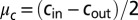 , and the horizontal lines are c and
  , respectively. The second eigenvalue
  is well-separated from the bulk throughout the detectable regime.
The eigenvector corresponding to  is strongly correlated with the communities. Because B is defined on directed edges, at each vertex we sum this eigenvector over all its incoming edges. If we label vertices according to the sign of this sum, then the majority of vertices are labeled correctly (up to a change of sign, which switches the two communities). Thus, a spectral algorithm based on B succeeds when
  , i.e., when 1 holds—but, unlike standard spectral algorithms, this criterion now holds even in the sparse case.
We present arguments for these claims in the next section. We will also see that the important part of B’s spectrum can be obtained from a  matrix (16, 25, 26)
 |
This lets us work with a 2n-dimensional matrix rather than a 2m-dimensional one, which significantly reduces the computational complexity of our algorithm.
Reconstruction and a Community-Correlated Eigenvector
In this section we sketch justifications of the claims in the previous section regarding B’s spectral properties, showing that its second eigenvector is correlated with the communities whenever 1 holds. We assume that  , so that the graph is locally tree-like.
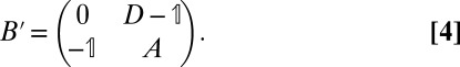
We start by explicitly constructing a vector g which is correlated with the communities and is an approximate eigenvector with eigenvalue  , as defined in Eq. 3. We follow ref. 11, which derived a similar result in the case of random regular graphs. For a given integer r, consider the vector
  defined by
 |
where  denotes u’s community, and
  denotes the number of steps required to go from
  to
to  in the graph of directed edges. By the theory of the reconstruction problem on trees (27, 28), if 1 holds, then for every
  , the correlation
  is bounded away from zero in the limit
  .
.
Next, we argue that if r is large then g is an approximate eigenvector of B with eigenvalue  . As long as the radius-r neighborhood of v is a tree, we have
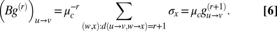 |
This is not precisely an eigenvalue equation because  ; however, it turns out that they are close with high probability. Indeed, we may write
  as
as
 |
Now, there are (in expectation)  terms in this sum, each of which, conditioned on the
  s, has mean zero and constant variance. Hence,
  . Summing over u and v, we have
  . If 1 holds then
  and so with high probability the error term tends to zero for large r. Because
  is bounded above zero, Eq. 6 then becomes
so  is indeed an approximate eigenvector for B with eigenvalue
  . Because, as we will discuss shortly, the bulk of B’s spectrum is bounded away from
  , it follows that the true eigenvector with eigenvalue
  is close to
  , and so it may be used for community detection. Specifically, if we label vertices according to the sign of this eigenvector (summed over all incoming edges at each vertex) we obtain the true communities with significant accuracy.
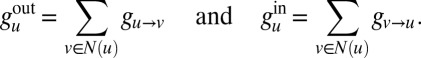
Summing over incoming and outgoing edges also lets us relate B’s spectrum to that of  (Eq. 4). Given a 2m-dimensional vector g, define
  and
and  as the n-dimensional vectors
 |
If we apply B to g, each incoming edge  contributes
  times to u’s outgoing edges. Similarly, each edge
  with
with  contributes to the incoming edge
  . As a result, we have
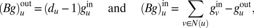 |
or more succinctly,
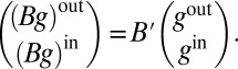 |
Now suppose that  . If
. If  and
and  are nonzero, then
  is an eigenvector of
  with the same eigenvalue μ. In that case, we have
so μ is a root of the quadratic eigenvalue equation
This equation is well known in the theory of graph zeta functions (16, 25, 26). It accounts for 2n of B’s eigenvalues, the other  of which are
  .
.
Next, we argue that the bulk of B’s spectrum is confined to the disk of radius  . First note that for any matrix B,
 |
On the other hand, for any fixed r, because G is locally tree-like in the limit  , each diagonal entry
  of
of  is equal to the number of vertices exactly r steps from v, other than those connected via u. In expectation this is
  , so by linearity of expectation
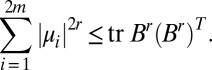
  . In that case, the 2rth moment in the spectral measure obeys
  .
.
Because this holds for any fixed r, we conclude that almost all of B’s eigenvalues obey  . Proving that all the eigenvalues in the bulk are asymptotically confined to this disk requires a more precise argument and is left for future work.
Finally, the singular values of B are easy to derive for any simple graph, i.e., one without self-loops or multiple edges. Namely, BBT is block-diagonal: for each vertex v, it has a rank-one block of size  that connects v’s outgoing edges to each other. As a consequence, B has n singular values
  , and its other
  singular values are 1. However, because B is not symmetric, its eigenvalues and its singular values are different—whereas its singular values are controlled by the vertex degrees, its eigenvalues are not. This is precisely why its spectral properties are better than those of A and related operators.
More than Two Groups and General Degree Distributions
The arguments given above regarding B’s spectral properties generalize straightforwardly to other graph ensembles. First, consider block models with q groups, where for  group a has fractional size
  . The average degree of group a is
  . The hardest case is where
  is the same for all a, so that we cannot simply label vertices according to their degree.
The leading eigenvector again has eigenvalue c, and the bulk of B’s spectrum is again confined to the disk of radius  . Now B has
  linearly independent eigenvectors with real eigenvalues, and the corresponding eigenvectors are correlated with the true group assignment. If these real eigenvalues lie outside the bulk, we can identify the groups by assigning a vector in
  to each vertex, and applying a clustering technique such as k means. These eigenvalues are of the form
  , where ν is a nonzero eigenvalue of the
  matrix
In particular, if  for all a, and
  for
for  , and
, and  for
for  , we have
  . The detectability threshold is again
  , or
, or
More generally, if the community-correlated eigenvectors have distinct eigenvalues, we can have multiple transitions where some of them can be detected by a spectral algorithm whereas others cannot.
There is an important difference between the general case and  . Whereas for
  it is literally impossible for any algorithm to distinguish the communities below this transition, for larger q the situation is more complicated. In general (for
  in the assortative case, and
  in the disassortative one) the threshold 9 marks a transition from an ‘‘easily detectable’’ regime to a ‘‘hard detectable’’ one. In the hard detectable regime, it is theoretically possible to find the communities, but it is conjectured that any algorithm that does so takes exponential time (9, 10). In particular, we have found experimentally that none of B’s eigenvectors are correlated with the groups in the hard regime. Nonetheless, our arguments suggest that spectral algorithms based on B are optimal in the sense that they succeed all of the way down to this easy–hard transition.
Because a major drawback of the stochastic block model is that its degree distribution is Poisson, we can also consider random graphs with specified degree distributions. Again, the hardest case is where the groups have the same degree distribution. Let  denote the fraction of vertices of degree k. The average branching ratio of a branching process that explores the neighborhood of a vertex, i.e., the average number of new edges leaving a vertex v that we arrive at when following a random edge, is
 |
We assume here that the degree distribution has bounded second moment so that this process is not dominated by a few high-degree vertices. The leading eigenvalue of B is  , and the bulk of its spectrum is confined to the disk of radius
  , even in the sparse case where
  does not grow with the size of the graph. If
  and the average numbers of new edges linking v to its own group and the other group are
  and
and  , respectively, then the approximate eigenvector described in the previous section has eigenvalue
  . The detectability threshold 1 then becomes
  , or
, or  . The threshold 9 for q groups generalizes similarly.
Deriving B by Linearizing Belief Propagation
The matrix B also appears naturally as a linearization of the update equations for belief propagation (BP). This linearization was used previously to investigate phase transitions in the performance of the BP algorithm (5, 9, 10, 29).
We recall that BP is an algorithm that iteratively updates messages  along the directed edges. These messages represent the marginal probability that a vertex v belongs to a given community, assuming that the vertex w is absent from the network. Each such message is updated according to the messages
  that v receives from its other neighbors
  . The update rule depends on the parameters
  and
and  of the block model, as well as the expected size of each community. For the simplest case of two equally sized groups, the BP update (9, 10) can be written as
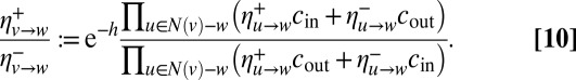 |
Here, + and − denote the two communities. The term  , where
  and
and  is the current estimate of the fraction of vertices in the two groups, represents messages from the nonneighbors of v. In the assortative case, it prevents BP from converging to a fixed point where every vertex is in the same community.
The update in Eq. 10 has a trivial fixed point  , where every vertex is equally likely to be in either community. Writing
  and linearizing around this fixed point gives the following update rule for δ:
 |
More generally, in a block model with q communities, an affinity matrix  , and an expected fraction
  of vertices in each community a, linearizing around the trivial fixed point and defining
  gives a tensor product operator
where T is the  matrix defined in Eq. 8.
This shows that the spectral properties of the nonbacktracking matrix are closely related to BP. Specifically, the trivial fixed point is unstable, leading to a fixed point that is correlated with the community structure, exactly when  has an eigenvalue greater than 1. However, by avoiding the fixed point where all of the vertices belong to the same group, we suppress B’s leading eigenvalue; thus the criterion for instability is
  , where v is T’s leading eigenvalue and
  is B’s second eigenvalue. This is equivalent to Eq. 9 in the case where the groups are of equal size.
In general, the BP algorithm provides a slightly better agreement with the actual group assignment, because it approximates the Bayes-optimal inference of the block model. On the other hand, the BP update rule depends on the parameters of the block model, and if these parameters are unknown they need to be learned, which presents additional difficulties (12). In contrast, our spectral algorithm does not depend on the parameters of the block model, giving an advantage over BP in addition to its computational efficiency.
Experimental Results and Discussion
In Fig. 4, we compare the spectral algorithm based on the nonbacktracking matrix B with those based on various classical operators: the adjacency matrix, modularity matrix, Laplacian, normalized Laplacian, and the random walk matrix. We see that there is a regime where standard spectral algorithms do no better than chance, whereas the one based on B achieves a strong correlation with the true group assignment all of the way down to the detectability threshold. We also show the performance of BP, which is believed to be asymptotically optimal (9, 10).
Fig. 4.

Accuracy of spectral algorithms based on different linear operators, and of BP, for two groups of equal size. (Left) We vary  while fixing the average degree
  ; the detectability transition given by 1 occurs at
  . (Right) We set
  and vary c; the detectability transition is at
  . Each point is averaged over 20 instances with
  . Our spectral algorithm based on the nonbacktracking matrix B achieves an accuracy close to that of BP, and both remain large all of the way down to the transition. Standard spectral algorithms (applied to the giant component of each graph, which contains all but a small fraction of the vertices) based on the adjacency matrix, modularity matrix, Laplacian, normalized Laplacian, and the random walk matrix all fail well above the transition, giving a regime where they do no better than chance.
We measure the performance as the overlap, defined as
 |
Here,  is the true group label of vertex u, and
  is the label found by the algorithm. We break symmetry by maximizing over all
  permutations of the groups. The overlap is normalized so that it is 1 for the true labeling, and 0 for a uniformly random labeling.
In Fig. 5 we illustrate clustering in the case  . As described above, in the detectable regime we expect to see
  eigenvectors with real eigenvalues that are correlated with the true group assignment. Indeed, B’s second and third eigenvectors are strongly correlated with the true clustering, and applying k means in
  gives a large overlap. In contrast, the second and third eigenvectors of the adjacency matrix are essentially uncorrelated with the true clustering, and similarly for the other traditional operators.
Fig. 5.

Clustering for three groups of equal size. (Left) Scatter plot of the second and third eigenvectors (X and Y axis, respectively) of the nonbacktracking matrix B, with colors indicating the true group assignment. (Right) Analogous plot for the adjacency matrix A. Here,  ,
,  , and
, and 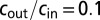 . Applying k means gives an overlap 0.712 using B, but 0.0063 using A.
Finally, we turn to real networks to illustrate the advantages of the nonbacktracking matrix in practical applications. In Fig. 6 we show B’s spectrum for several networks commonly used as benchmarks for community detection. In each case we plot a circle whose radius is the square root of the largest eigenvalue. Even though these networks were not generated by the stochastic block model, these spectra look qualitatively similar to the picture discussed above (Fig. 2). This leads to several very convenient properties. For each of these networks we observed that only the eigenvectors with real eigenvalues are correlated to the group assignment given by the ground truth. Moreover, the real eigenvalues that lie outside of the circle are clearly identifiable. This is very unlike the situation for the operators used in standard spectral clustering algorithms, where one must decide which eigenvalues are in the bulk and which are outside.
Fig. 6.
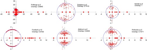
Spectrum of the nonbacktracking matrix in the complex plane for some real networks commonly used as benchmarks for community detection, taken from refs. 30–35. The radius of the circle is the square root of the largest eigenvalue, which is a heuristic estimate of the bulk of the spectrum. The overlap is computed using the signs of the second eigenvector for the networks with two communities, and using k means for those with three and more communities. The nonbacktracking operator detects communities in all these networks, with an overlap comparable to the performance of other spectral methods. As in the case of synthetic networks generated by the stochastic block model, the number of real eigenvalues outside the bulk appears to be a good indicator of the number q of communities.
In particular, the number of real eigenvalues outside the circle seems to be a natural indicator for the true number of clusters in the network, just as for networks generated by the stochastic block model. This suggests that in the network of political books there might be 4 groups rather than 3, in the blog network there might be more than 2 groups, and in the NCAA football network there might be 10 groups rather than 12. However, we note that some real eigenvalues may correspond to small cliques.
A Matlab implementation with demos that can be used to reproduce our numerical results can be found at http://panzhang.net/dea/dea.tar.gz.
Conclusion
Although recent advances have made statistical inference of network models for community detection far more scalable than in the past (e.g., refs. 9, 24, 36, 37), spectral algorithms are highly competitive because of the computational efficiency of sparse linear algebra. However, for sparse networks there is a large regime in which statistical inference methods such as BP can detect communities, whereas standard spectral algorithms cannot.
We closed this gap by using the nonbacktracking matrix B as a starting point for spectral algorithms. We showed that for sparse networks generated by the stochastic block model, B’s spectral properties are much better than those of the adjacency matrix and its relatives. In fact, it is asymptotically optimal in the sense that it allows us to detect communities all of the way down to the detectability transition. We also computed B’s spectrum for some real-world networks, showing that the real eigenvalues are a good guide to the number of communities and the correct labeling of the vertices.
Our approach can be straightforwardly generalized to spectral clustering for other types of sparse data, such as weighted graphs with real-valued similarities  between vertices: then
  if
if  and
and  , and 0 otherwise. We believe that, as for sparse graphs, there will be important regimes in which using B will succeed where standard clustering algorithms fail. Given the wide use of spectral clustering throughout the sciences, we expect that the nonbacktracking matrix and its generalizations will have a significant impact on data analysis.
Acknowledgments
We are grateful to Noga Alon, Brian Karrer, Michael Krivelevich, Mark Newman, Nati Linial, Yuval Peres, and Xiaoran Yan for helpful discussions. C.M. and P.Z. are supported by Air Force Office of Scientific Research and Defense Advanced Research Planning Agency under Grant FA9550-12-1-0432. F.K. and P.Z. have been supported in part by the European Research Council under the European Union’s 7th Framework Programme Grant Agreement 307087-SPARCS. E.M. and J.N. were supported by National Science Foundation (NSF) Department of Mathematical Sciences Grant 1106999 and Department of Defense Office of Naval Research Grant N000141110140. E.M was supported by NSF Grant Computing and Communication Foundation 1320105.
Footnotes
The authors declare no conflict of interest.
*This Direct Submission article had a prearranged editor.
References
- 1.Holland PW, Laskey KB, Leinhardt S. Stochastic blockmodels: First steps. Soc Networks. 1983;5(2):109–137. [Google Scholar]
- 2.Wang YJ, Wong GY. Stochastic blockmodels for directed graphs. J Am Stat Assoc. 1987;82(397):8–19. [Google Scholar]
- 3.Von Luxburg U. A tutorial on spectral clustering. Stat Comput. 2007;17(4):395–416. [Google Scholar]
- 4.Bickel PJ, Chen A. A nonparametric view of network models and Newman-Girvan and other modularities. Proc Natl Acad Sci USA. 2009;106(50):21068–21073. doi: 10.1073/pnas.0907096106. [DOI] [PMC free article] [PubMed] [Google Scholar]
- 5.Coja-Oghlan A, Mossel E, Vilenchik D. A spectral approach to analyzing belief propagation for 3-coloring. Combin Probab Comput. 2009;18(6):881–912. [Google Scholar]
- 6.Coja-Oghlan A. Graph partitioning via adaptive spectral techniques. Combin Probab Comput. 2010;19(02):227–284. [Google Scholar]
- 7.McSherry F. 2001. Spectral partitioning of random graphs. Proceedings of 42nd Foundations of Computer Science (IEEE Computer Society, Las Vegas), pp 529–537.
- 8.Nadakuditi RR, Newman MEJ. Graph spectra and the detectability of community structure in networks. Phys Rev Lett. 2012;108(18):188701. doi: 10.1103/PhysRevLett.108.188701. [DOI] [PubMed] [Google Scholar]
- 9.Decelle A, Krzakala F, Moore C, Zdeborová L. Inference and phase transitions in the detection of modules in sparse networks. Phys Rev Lett. 2011;107(6):065701. doi: 10.1103/PhysRevLett.107.065701. [DOI] [PubMed] [Google Scholar]
- 10.Decelle A, Krzakala F, Moore C, Zdeborová L. Asymptotic analysis of the stochastic block model for modular networks and its algorithmic applications. Phys Rev E Stat Nonlin Soft Matter Phys. 2011;84(6 Pt 2):066106. doi: 10.1103/PhysRevE.84.066106. [DOI] [PubMed] [Google Scholar]
- 11.Mossel E, Neeman J, Sly A. 2012. Stochastic block models and reconstruction. arXiv:1202.1499v4.
- 12.Zhang P, Krzakala F, Reichardt J, Zdeborová L. Comparative study for inference of hidden classes in stochastic block models. J Stat Mech. 2012;12:P12021. Available at http://iopscience.iop.org/1742-5468/2012/12/P12021. Accessed November 14, 2013. [Google Scholar]
- 13.McKay BD. The expected eigenvalue distribution of a large regular graph. Linear Algebra Appl. 1981;40:203–216. [Google Scholar]
- 14.Sodin S. Random matrices, nonbacktracking walks, and orthogonal polynomials. J Math Phys. 2007;48:123503. [Google Scholar]
- 15.Friedman J. A proof of Alon’s second eigenvalue conjecture and related problems. Memoirs of the American Mathematical Society. 2008;195(910) [Google Scholar]
- 16.Hashimoto K. Zeta functions of finite graphs and representations of p-adic groups. Advanced Studies in Pure Mathematics. 1989;15:211–280. [Google Scholar]
- 17.Alon N, Benjamini I, Lubetzky E, Sasha S. Non-backtracking random walks mix faster. Commun Contemp Math. 2007;9(4):585–603. [Google Scholar]
- 18.Watanabe Y, Fukumizu K. 2010. Graph zeta function in the Bethe free energy and loopy belief propagation. arXiv:1002.3307.
- 19.Vontobel PO. 2010. Connecting the Bethe entropy and the edge zeta function of a cycle code. Proceedings of the International Symposium on Information Theory (IEEE, New York), pp 704–708.
- 20.Ren P, Wilson RC, Hancock ER. Graph characterization via Ihara coefficients. IEEE Trans Neural Netw. 2011;22(2):233–245. doi: 10.1109/TNN.2010.2091969. [DOI] [PubMed] [Google Scholar]
- 21.Wigner EP. On the distribution of the roots of certain symmetric matrices. Ann Math. 1958;67(2):325–327. [Google Scholar]
- 22.Krivelevich M, Sudakov B. The largest eigenvalue of sparse random graphs. Combin Probab Comput. 2003;12(01):61–72. [Google Scholar]
- 23.Bollobas B, Svante J, Oliver R. The phase transition in inhomogeneous random graphs. Random Structures Algorithms. 2007;31(1):3–122. [Google Scholar]
- 24.Amini AA, Chen A, Bickel PJ, Levina E. 2012. Pseudolikelihood methods for community detection in large sparse networks. arXiv:1207.2340.
- 25.Bass H. The Ihara-Selberg zeta function of a tree lattice. Int J Math. 1992;3(06):717–797. [Google Scholar]
- 26.Angel O, Friedman J, Hoory S. 2007. The non-backtracking spectrum of the universal cover of a graph. arXiv:0712.0192.
- 27.Kesten H, Stigum BP. Additional limit theorems for indecomposable multidimensional Galton-Watson processes. Ann Math Stat. 1966;37(6):1463–1481. [Google Scholar]
- 28.Mossel E, Peres Y. Information flow on trees. Ann Appl Probab. 2003;13:817–844. [Google Scholar]
- 29.Richardson T, Urbanke R. Modern Coding Theory. Cambridge, UK: Cambridge Univ Press; 2008. [Google Scholar]
- 30.Adamic L, Glance N. 2005. The political blogosphere and the 2004 US Election: Divided they blog. Proceedings of the 3rd International Workshop on Link Discovery (Association for Computing Machinery, New York), pp 36–43.
- 31.Zachary WW. An information flow model for conflict and fission in small groups. J Anthropol Res. 1977;33:452–473. [Google Scholar]
- 32.Newman MEJ. Finding community structure in networks using the eigenvectors of matrices. Phys Rev E Stat Nonlin Soft Matter Phys. 2006;74(3 Pt 2):036104. doi: 10.1103/PhysRevE.74.036104. [DOI] [PubMed] [Google Scholar]
- 33.Girvan M, Newman MEJ. Community structure in social and biological networks. Proc Natl Acad Sci USA. 2002;99(12):7821–7826. doi: 10.1073/pnas.122653799. [DOI] [PMC free article] [PubMed] [Google Scholar]
- 34.Lusseau D, et al. The bottlenose dolphin community of Doubtful Sound features a large proportion of long-lasting associations. Behav Ecol Sociobiol. 2003;54(4):396–405. [Google Scholar]
- 35. Krebs V (2012) Social Network Analysis software & services for organizations, communities, and their consultants. Available at www.orgnet.com/. Accessed November 14, 2013.
- 36.Ball B, Karrer B, Newman MEJ. Efficient and principled method for detecting communities in networks. Phys Rev E Stat Nonlin Soft Matter Phys. 2011;84(3 Pt 2):036103. doi: 10.1103/PhysRevE.84.036103. [DOI] [PubMed] [Google Scholar]
- 37.Gopalan P, Mimno D, Gerrish S, Freedman M, Blei D. 2012. Scalable inference of overlapping communities. Advances in Neural Information Processing Systems 25, eds Bartlett P, Pereira FCN, Burges CJC, Bottou L, Weinberger KQ, pp 2258–2266. [Google Scholar]