Artificial Pancreas: Model Predictive Control Design from Clinical Experience

Abstract

Background

The objective of this research is to develop a new artificial pancreas that takes into account the experience accumulated during more than 5000 h of closed-loop control in several clinical research centers. The main objective is to reduce the mean glucose value without exacerbating hypo phenomena. Controller design and in silico testing were performed on a new virtual population of the University of Virginia/Padova simulator.

Methods

A new sensor model was developed based on the Comparison of Two Artificial Pancreas Systems for Closed-Loop Blood Glucose Control versus Open-Loop Control in Patients with Type 1 Diabetes trial AP@home data. The Kalman filter incorporated in the controller has been tuned using plasma and pump insulin as well as plasma and continuous glucose monitoring measures collected in clinical research centers. New constraints describing clinical knowledge not incorporated in the simulator but very critical in real patients (e.g., pump shutoff) have been introduced. The proposed model predictive control (MPC) is characterized by a low computational burden and memory requirements, and it is ready for an embedded implementation.

Results

The new MPC was tested with an intensive simulation study on the University of Virginia/Padova simulator equipped with a new virtual population. It was also used in some preliminary outpatient pilot trials. The obtained results are very promising in terms of mean glucose and number of patients in the critical zone of the control variability grid analysis.

Conclusions

The proposed MPC improves on the performance of a previous controller already tested in several experiments in the AP@home and JDRF projects. This algorithm complemented with a safety supervision module is a significant step toward deploying artificial pancreases into outpatient environments for extended periods of time.

J Diabetes Sci Technol 2013;7(6):1470-1483

Introduction

An artificial pancreas (AP) is an automatic device for regulating glucose in diabetes patients. A new perspective for the development of a device suitable for outpatient use started with the availability of subcutaneous (SC) glucose sensors and SC insulin pumps. The integration of these two components with a control algorithm is called the AP. In particular, in 1999, MiniMed introduced a commercial continuous glucose monitoring (CGM) system. Since then, several research projects studied and experimented with AP systems, starting with the MiniMed AP project,¹ with an acceleration caused by the launch of research projects funded by the JDRF, the European Commission, and the National Institutes of Health.^2–6

Designing a control algorithm for the SC-to-SC glucose–insulin system is challenging, because the system is characterized by significant interindividual variability, time-varying dynamics, nonlinear phenomena, and time delays due to the absorption of insulin from the SC level to the blood and, in reverse, of glucose from the blood to the SC level. Moreover, the glucose profile depends on the insulin, whose delivery is bounded not only within an interval ranging from zero to a maximal value imposed by the pump, but also on very important disturbances such as meals and physical exercise that may be predicted to some extent.

The objective of the control algorithm is to keep the glucose levels within an optimal range (70–140 mg/dl). In the literature, several algorithms have been presented starting from proportional-integral-derivative schemes^1,7 and, more recently, relying on a very promising approach called model predictive control (MPC).^2,8–18 So far, encouraging pilot results have been reported using proportional-integral-derivative control^1,3 and MPC strategies.^4,6,19 In Breton and coauthors,²⁰ the MPC algorithm described by Patek and coauthors¹⁸ was in vivo tested. A comparison of two MPC-based artificial pancreas systems was performed by Luijf and coauthors.²¹ The study was performed on 48 patients with type 1 diabetes and consisted of three randomized 24 h admissions (with 23 h of closed-loop control in two of the admissions and one control admission with open loop) to the clinical research center. One of the closed-loop controls is the iAP (or International Artificial Pancreas Study Group) control algorithm, developed following the modular architecture proposed by Patek and coauthors¹⁸ that includes the MPC algorithm described by Soru and coauthors,¹⁰ herein called MPC1, and the safety supervision module (SSM) described by Hughes and coauthors.²² In this article, a new MPC version, herein called MPC2, was designed based on collected data and other clinical experiences. The results illustrated in this article were tested in silico using the simulator developed by the Universities of Padova and Virginia equipped with a new cohort of virtual subjects that span sufficiently well the interindividual variability of key metabolic parameters in the general population of diabetes patients (see the work of Dalla Man and coauthors²³).

Methods

The MPC1 algorithm takes advantage of the knowledge of conventional therapy that addresses glucose regulation by a mix of piecewise constant insulin infusion, also called basal insulin, u_b, and impulse-like injections that are made just before meals to prevent excessive rises of blood glucose (BG), also called insulin bolus, u_bolus. In the absence of meals, the basal insulin, which varies from patient to patient, would eventually bring BG to a steady-state value, called basal glucose, G_b. The amount of the insulin bolus is scaled to the meal size using the patient parameters carbohydrate-to-insulin ratio and correction factor.

MPC1 is the linear model predictive control (LMPC) described by Soru and coauthors¹⁰ that uses an approximate linear model of the insulin–glucose dynamics obtained from the linearization around a suitable working point of the more complex nonlinear model reported in by Magni and coauthors.⁹ The derived linearized model can be written in the following form:

$$\{\begin{array}{c}x\left(k+1\right)=Ax\left(k\right)+Bu\left(k\right)+Md\left(k\right)\\ y\left(k\right)=Cx\left(k\right)\end{array},$$ (1)

where x(k) ∈ R¹³ is the state as reported in Table 1 , y(k) = CGM(k) – G_b (mg/dl) is the difference between the SC glucose and the basal value (G_b), u(k) = i(k) – u_b(k) (pmol/kg) is the difference between the injected insulin and its reference value (normalized by the patient weight), and d(k) (mg) represents the meal.

Table 1.

Table of State Vector x(k) of the Dalla Man Model reported by Magni and Coauthors⁹

State	Description	Units
x1	Glucose into the stomach in solid phase	mg
x2	Glucose into the stomach in liquid phase	mg
x3	Glucose into the intestine	mg
x4	Plasma glucose	mg/kg
x5	Tissues glucose	mg/kg
x6	Plasma insulin	pmol/kg
x7	Insulin action	pmol/liter
x8	Insulin action delay on glucose production	pmol/liter
x9	Delayed insulin	pmol/liter
x10	Insulin in the liver	pmol/kg
x11	First compartments of SC insulin	pmol/kg
x12	Second compartments of SC insulin	pmol/kg
x13	SC glucose	mg/kg

Thereafter, it is assumed that the triplet (A, B, C) is both stabilizable and detectable. The LMPC algorithm uses this model to predict the future glucose profile given the carbohydrates and insulin taken in by the patient.

The cost function is a quadratic penalty defined as

$$J\left(x\right(k),u(\cdot ),k)=\sum _{i=0}^{N-1}{\left(q\right(y(k+i))-y_0(k+i\left)\right)}^2+{\left(u\right(k+i)-u_0(k+i\left)\right)}^2+\Vert x(k+N){\Vert }_P^2$$ (2)

where q is the positive scalar weight and N is the prediction horizon. Moreover, ∣∣ x(k + N)∣∣ _P = x(k + N)’Px(k + N), where P is the unique nonnegative solution of the discrete time Riccati equation:

$$P=A^{\prime }PA+q{C}^{\prime }C-A^{\prime }PB\left(1+B^{\prime }PB\right)B^{\prime }PA$$

The reference signals are defined as y_o(k) = y˜(k) – G_b (mg/dl), the difference between the reference value (y˜) of the SC glucose and the glucose basal value (G_b), and u_o(t) = ũ(k) – u_b(k) (pmol/kg), the difference between the reference value (ũ) of the insulin profile and the insulin basal value (u_b), normalized by the patient weight.

The control law associated with a constrained LMPC may be derived either by solving an on-line quadratic programming problem or through a multiparametric approach, whose result is a piecewise constant control law that can be computed offline.

However, in view of the restrictive regulatory constraint and the significant uncertainty in the model, and in order to avoid online optimization or the computational and memory burdens of an explicit MPC for constrained systems, the proposed algorithm does not include explicit constraints. Hence it is possible to calculate the closed-form solution:

$$u^{MPC}\left(k\right)=\left[1\hspace{0.17em}\hspace{0.17em}\hspace{0.17em}0\hspace{0.17em}\hspace{0.17em}\hspace{0.17em}\cdots \hspace{0.17em}\hspace{0.17em}0\right]\left(-K_{x}x\left(k\right)-k_{d}D\left(k\right)+K_{Y_0}{Y}_0\left(k\right)+K_{U_0}{U}_0\left(k\right)\right),$$ (3)

where K_x ∈ R^Nx13, K_d ∈ R^NxN, K_Y0 ∈ R^NxN, K_U0 ∈ R^NxN are derived as described in by Soru and coauthors¹⁰ and

$$D\left(k\right)=\left[d\left(k\right)\hspace{0.17em}\hspace{0.17em}\hspace{0.17em}\cdots d\left(k+N-2\right)\hspace{0.17em}\hspace{0.17em}d\left(k+N-1\right)\right]\prime$$

is the vector of future meals and

$$\begin{array}{l}{Y}_0\left(k\right)=\left[y_0\left(k+1\right)\hspace{0.17em}\hspace{0.17em}\cdots y_0\left(k+N-1\right)0\right]\prime \\ U_0\left(k\right)=\left[u_0\left(k\right)\cdots u_0\left(k+N-2\right)u_0\left(k+N-1\right)\right]\prime \end{array}$$

In general, the state x(k) of the model is not accessible, so a Kalman filter is used to estimate it. The Kalman filter improves the quality of the information provided to the LMPC algorithm, exploiting the knowledge included in the model as well as the past injected insulin. In fact, the Kalman filter is used to update the estimated glucose–insulin state using past information about glucose, insulin, and carbohydrates. The linear system (Equation 1), affected by noises, is written as

$$\{\begin{array}{c}x\left(k+1\right)=Ax\left(k\right)+Bu\left(k\right)+Md\left(k\right)+v_x\left(k\right)\\ y\left(k\right)=Cx\left(k\right)+v_y\left(k\right)\end{array}$$

where v = [v_x v_y] is a multivariate zero-mean white Gaussian noise with covariance matrix

$$V=\left[\begin{array}{cc}{Q}_{KF}& 0\\ 0& R_{KF}\end{array}\right],Q_{KF}>0\hspace{0.17em}{R}_{KF}>0,$$

and the initial state x₀ = x(0) is assumed to be a zero mean Gaussian random variable independent of v.

From clinical data collected during the Comparison of Two Artificial Pancreas Systems for Closed-Loop Blood Glucose Control versus Open-Loop Control in Patients with Type 1 Diabetes (CAT) AP@home trial reported by Luijf and coauthors,²¹ three major problems were pointed out: a measurement error larger than the one assumed for Kalman filter tuning, a virtual population used for controller synthesis whose insulin sensitivity was underestimated, and too-high nocturnal glucose levels.

New Measurement Error Model Derived from CAT AP@home

From the 141 data sets relative to the 47 patients enrolled in the CAT AP@home trial, information about BG and CGM was extracted. The BG sampling time was 15 min, with exception of the evening hours when it was decreased to 30 min and the night when it was 60 min. The CGM was sampled with the Dexcom Seven^® Plus every 5 min. A critical point in the synthesis of a closed-loop controller is the quality of the measurement error model. The University of Virginia/Padova simulator,²⁴ used to tune the MPC by Soru and coauthors,¹⁰ includes the error model proposed by Breton and Kovatchev²⁵ consisting of an autoregressive [AR(1)] model and a nonlinear Johnson function. In order to evaluate the capability of the measurement error model to describe the real difference between SC glucose concentration and CGM, the scheme reported in Figure 1 is first introduced. The relation between BG and interstitial glucose is modeled as a first-order system with time constant t, which is representative of the lag between the blood and SC glucose concentrations. As constant t is unknown and patient dependent, a sensitivity analysis of ê with respect to t is made by considering the latter as a lognormal stochastic variable with mean 10.27 [s] and variance 7.18 [s²] . The estimate of the measurement error ê is compared with the modeled error ê_M through the visual predictive check approach.²⁶ The visual predictive check representation of ê and ê_M obtained through the model proposed by Breton and Kovatchev,²⁵ reported in Figure 2A, shows that the variability of the measurement error is significantly underestimated. Some limitations of this model error are already pointed out by Facchinetti and coauthors,²⁷ and thanks to the availability of four simultaneous sensor data, a new description of the components of the sensor model error has been proposed by Facchinetti and coauthors.²⁸ Here a new autoregressive [AR(2)] model is identified in order to describe the total measurement error, including wearing issues in addition to noise and drift usually considered.

Figure 1.

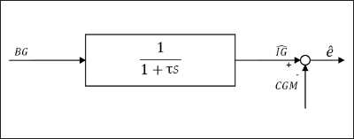
Estimation of measurement error ê. IG is an estimate of the SC glucose concentration interstitial glucose, CGM represents its measure, and ê is an estimate of the measurement error.

Figure 2.

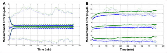
Visual predictive check representation of 10th and 90th percentiles, estimation of measurement error ê with τ variation effect (continuous line), and modelled error ê_M with different realizations (plus marker). Top panel (A) Comparison between the measurement error ê and the error model.²⁵ Bottom panel (B) Comparison between the measurement error ê and the new error model.

The new model can be described by

$${\text{ε}}_{pV}\left(k\right)=a_1\cdot {\text{ε}}_{pV}\left(k-1\right)+a_2\cdot \hspace{0.17em}{\text{ε}}_{pV}\left(k-2\right)+v\left(k\right),$$

where error v(k) is a Gaussian white noise with mean m_v and variance ${\sigma }_v^2$, parameters a₁ and a₂ are coefficients of the autoregressive model, and the distribution of the initial states of the process is normal with mean m_is and variance

$${\text{σ}}_{is}^2$$

(see Table 2).

Table 2.

Values of the Autoregressive Model of the Sensor Noise ε_PV²¹

Parameter	Value	Units
a1	1.5458	Adimensional
a2	−0.5708	Adimensional
μv	0.0017	mmol/liter
${\text{σ}}_v^2$v2	0.0283	mmol2/liter2
μis	[−0.1766 −0.1566]	mmol/liter
${\text{σ}}_{is}^2$	$\left[\begin{array}{cc}0.7759& 0.7895\\ 0.7895& 0.8603\end{array}\right]$	mmol2/liter2

The results obtained with the new model are presented in Figure 2B. Also, the mean absolute relative difference (MARD)²⁹ between CGM and BG obtained with the model (median 15%, interquartile range 13–17%) is in agreement with the data collected during the CAT AP@ home trial (median 12%, interquartile range 10–18%); it is also similar to the MARD obtained with the Dexcom Seven Plus by Christiansen and coauthors²⁹ (median 14%, interquartile range 12–20%). In order to use this model with other sensors, variance s_v² must be adapted. For example, with s_v² = 0.0141, the MARD is 11% with interquartile range 10–13%, similar to that of the Dexcom G4 (median 12.5%, interquartile range 9–16%) reported by Christiansen and coauthors.²⁹

Model Predictive Control Retuning

The MPC algorithm was improved by exploiting the experience gained with the AP@home experiments. The main changes in the MPC2 algorithm are listed and described as follows:

1. refined basal/bolus reference therapy

2. meal bolus limitation

3. insulin constraint

4. pump shutoff avoidance

5. insulin variation constraint

6. retuning of the cost function using a new virtual population of patients and the new sensor noise model

Refined Basal/Bolus Reference Therapy

The reference value (ũ) included in the cost function was previously computed as

$$\tilde{u}\left(k\right)=\frac{\text{d}\left(\text{k}\right)}{CR}+u_b\left(k\right).$$

Here it is adapted considering also the patient’s BG concentration at the time of meal acknowledgement. Specifically, the correction, which is limited to percentage μ of the nominal meal bolus value, is computed as

$$\tilde{u}\left(k\right)=\frac{\text{d}\left(\text{k}\right)}{CR}+min\left(\text{μ}\cdot \frac{\text{d}\left(\text{k}\right)}{CR},\frac{\text{BG}-y_{target}}{CF}\right)+u_b\left(k\right)=u_{bolus}\left(k\right)+u_b\left(k\right)$$

where y_target is the glucose reference and m is the maximum allowed meal bolus correction.

Meal Bolus Limitation

A limitation on the maximum bolus deliverable for each meal is also introduced: a maximal a% of the nominal bolus can be suggested to compensate for the meal. In formal terms, Equation (3) was modified as

$$u^I\left(k\right)=\left[1\hspace{0.17em}\hspace{0.17em}0\hspace{0.17em}\hspace{0.17em}\cdots \hspace{0.17em}\hspace{0.17em}0\right]\left(-K_{x}x\left(k\right)+K_{Y_0}{Y}_0\left(k\right)+min\left(\frac{\alpha }{100}\cdot {\tilde{u}}_{bolus}\left(k\right),-K_{d}D\left(k\right)+K_{u_0}{U}_0\left(k\right)\right)\right),$$

Insulin Constraint

Due to the unconstrained nature of the MPC1, the finite horizon optimal solution can include negative insulin suggestions that obviously cannot be applied in the future. Hence the following constraint was introduced:

$$u^{II}\left(k\right)=u^I\left(k\right)+min\left({\displaystyle {\sum }_{i=1}^{N_i-1}\left(u^I\left(k+i\right)+u_b\right)}-\frac{\text{β}}{100}\ast u_b\ast \left(N_i-1\right),0\right),$$

where N_i is the considered horizon. This formula limits the suggested insulin, allowing also the possibility to suggest at least a percentage b of the basal in the future. In order to limit the MPC action, the control variable was also saturated according to the following rule:

$$u^{III}\left(k\right)=\left(max-u_b\left(k\right),min\left(\frac{\alpha }{100}\cdot {\tilde{u}}_{bolus}\left(k\right)-{\displaystyle {\sum }_{n=1}^{N_v}i\left(k-n\right)},u^{II}\left(k\right)\right)\right),$$

where i is the insulin effectively injected in the past and N_v is the considered horizon.

Pump Shutoff Avoidance

In the literature, it is widely documented that the absence of insulin delivery for a long period can lead to metabolic decompensation and diabetic ketoacidosis.³⁰ However, short-interval interruption of basal insulin infusion may also result in risks of ketosis.³¹ In order to avoid these events, a new constraint was added:

$$u^{IV}\left(k\right)=\{\begin{array}{cc}{u}^{III}\left(k\right)& \text{if}\hspace{0.17em}{G}_p\left(k\right)<\stackrel{-}{G}\\ max\left(u^{III}\right(k),{\text{γu}}_b(k\left)\right)& \text{otherwise}\end{array},$$

where γ is the guaranteed fraction of basal delivery in the future and Ḡ is a switching threshold.

Insulin Variation Constraint

Finally, data analysis showed that spikes in CGM can cause excessive reaction of the control algorithm. Hence, in order to avoid an increase of the suggested insulin greater than ζu_b the MPC suggestion was corrected as

$$u^{MPC}\left(k\right)=min\hspace{0.17em}\left(u^{IV}\right(k),i(k-1)-u_b(k-1)+\text{ζ}\cdot {\text{u}}_b(k\left)\right).$$

Meal boluses can violate this constraint.

Retuning of the Cost Function Using a New Virtual Population of Patients and the NewSensor Noise Model

Glucose profiles observed in the AP@home trials exhibited a relatively high glucose average (148.21 ± 20.42); therefore the glucose set point (ñy) was decreased. Moreover, the prediction horizon was shortened for embedded implementation.³² This is possible without performance degradation in view of the terminal penalty in Equation (2) that approximates the infinite horizon cost. Finally, the cost function was retuned following the procedure described by Soru and coauthors¹⁰ using the new virtual population²³ and the sensor model described in this work.

Kalman Filter Retuning

In order to improve the predictions of the Kalman filter, a retuning of the Q_KF and R_KF matrices, exploiting both the AP@home data and the new sensor error model, was implemented. Q_KF was set as a diagonal matrix whose entries q_i are gathered in five homogeneous groups taking the same values (see Table 3).

Table 3.

Grouping of Covariance Matrix Q_KF Diagonal Elements qi and Their Chosen Values

Group	Element	Signals	Value
1	q1, q2, q3	states in mg	0.1
2	q4, q5	states in mg/kg	10
3	q6, q7, q8	states in pmol/liter	0.1
4	q9, q10, q11, q12	states in pmol/kg	0.1
5	q13	state in mg/dl	10

Noise covariance matrix R_KF was set equal to the variance of signal v(k) (described in this article) while process noise covariance matrix Q_KF was tuned by minimizing the sum of the prediction error defined as

$$J_{ep}=(I_P-{\widehat{I}}_p)+\text{η}\cdot (\text{BG}-\widehat{\text{ΒG}}),$$

where I_p is the measured plasma insulin, Î_p is the plasma insulin estimated by the Kalman filter, $\widehat{\text{BG}}$ is the measured plasma glucose, BG is the plasma glucose estimated by the Kalman filter, and h is a suitable weight. The optimization was performed by an exhaustive research over a grid that considered for each q_i three possible values: 0.1, 1, and 10. The optimal values are reported in the last column of Table 3.

Results and Discussion

This section reports the in silico comparison between the MPC1 algorithm, used in the CAT AP@home trial,¹⁰ and MPC2, proposed in this article, with the parameters set as follows:

$$N=N_i=N_v=4,\hspace{0.17em}\text{μ=0}\mathrm{.25,}\hspace{0.17em}\hspace{0.17em}\hspace{0.17em}\tilde{y}=119\text{mg/dl,}\hspace{0.17em}\hspace{0.17em}{y}_{target}=115\hspace{0.17em}\text{mg/dl,}\hspace{0.17em}\text{α=120,}\hspace{0.17em}\text{β=50,}\hspace{0.17em}\hspace{0.17em}\text{γ=0}\mathrm{.3,}\overline{G}=140\hspace{0.17em}\text{mg/dl,}\hspace{0.17em}\text{ζ=3}.$$

The control weight q in Equation (2) is individualized using body weight, BW, and carbohydrate-to-insulin ratio as

$$q=e^{\left(-0.0366\cdot BW-0.2149\cdot CR+2.5444\right)},$$

where the coefficients were computed through the procedure described by Soru and coauthors¹⁰ applied to 50 virtual patients.

Three different scenarios were evaluated: a nominal one in which all parameters were known, a sensitivity variation scenario where a ±25% variation was randomly applied to the insulin sensitivity of each in silico patient in order to represent possible uncertainty on individual insulin sensitivity, and a meal variation scenario where the ingested amount of carbohydrates is the nominal one multiplied by a random factor uniformly distributed in [0.5 1.5] in order to reproduce a possible error in meal amount calculation. Each simulation started at 06:00 and lasted 34 h. Five meals were administrated during the whole trial: breakfast at 07:00 (50 g), lunch at 12:00 (60g), dinner at 18:30 (80g), and second breakfast and second lunch equal to the previous. In all scenarios, four sensor calibrations were planned per day: 30 min before each meal (06:30, 11:30, and 18:00) and one before the night (23:00). The comparison reported here was performed with the new virtual population²² composed of 100 adult patients and the sensor noise model presented in this work.

Differences in outcomes measures is assessed according with data distribution as reported in Table 4 .

Table 4.

Tests Used to Assert Signifcant Diference According to Data Distribution^a

	Data distributions
	Both Gaussian	At least one not Gaussian
Homoscedastic	Two-sample t-test33	Wilcoxon rank sum34
Not homoscedastic	Two-sample t-test with Satterthwaite’s approximation33

^aGaussianity and homoscedasticity and addressed by the Lilliefors test³⁵ and two-sample F-test,³⁴ respectively.

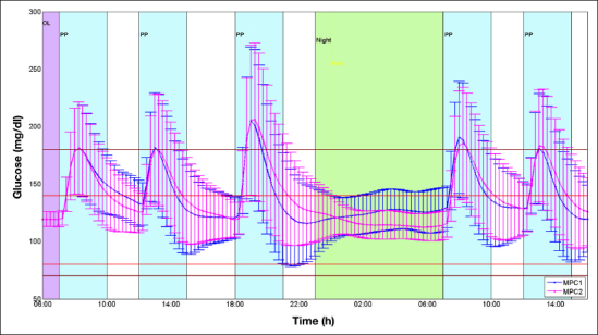
Figure 3 shows the results in terms of glucose profiles obtained with both algorithms in the nominal scenario: the glucose mean with MPC2 tends to the set point in the nocturnal period; moreover, lower excursions in the postprandial periods that cause hypoglycemia phenomena with MPC1 are reduced. MPC1 acts too aggressively after meals and maintains a high glucose level during the night. Figure 4 shows the improvement obtained with the new algorithm on an improved version of the classic control variability grid analysis (CVGA).³⁶ This improved version was introduced Soru and coauthors¹⁰ by allowing the classic CVGA nine square zones, associated with different control performance, to become concentric rings zones ranging from A to D. Axis scales and hence subject position remain the same. This new CVGA removes the limitation that a patient could move to a better zone with a slight reduction of one of the coordinates even at the cost of a substantial increase of the other one. Another feature is that all patients suffering from severe hypoglycemic or hyperglycemic episodes will fall in region D. For example, the subjects with minimum BG = 110 and maximum BG = 181 and minimum BG = 95 and maximum BG = 179 are in the B and A zones, respectively, with the square zones while they are both in the B zone with the ring zones; on the contrary, the subjects with minimum BG = 110 and maximum BG = 170 and minimum BG = 95 and maximum BG = 170 are placed in different zones with the ring zones (A versus B zone) but not with the square ones (A versus A zone); the subjects with minimum BG = 60 and maximum BG = 181 and minimum BG = 40 and maximum BG = 179 with the ring zones are, respectively, in the C and D zones, while with the square zones are in D and C zones, respectively.

Figure 3.

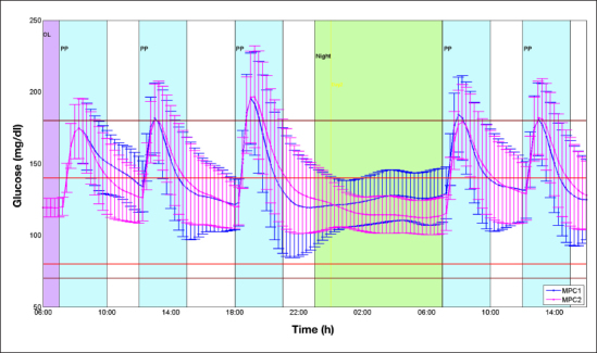
The figure shows for MPC1 (blue) and MPC2 (magenta) the mean (dots) and the variability (±standard deviation) of the glucose profiles obtained in 100 virtual patients with the nominal scenario. OL, open loop; PP, postprandial period.

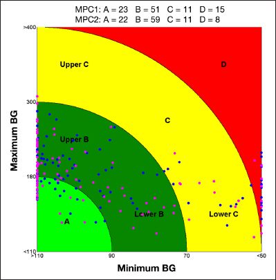
Figure 4.

The CVGA representing the results obtained using MPC1 (blue) and MPC2 (magenta) on the nominal scenario. Each point represents the coordinates (x is a function of the minimal glucose value and y a function of the maximal value) associated with a single patient.

The same considerations can be deduced from the analysis of the glucose profile obtained with the sensitivity variation scenario (see Figure 5) and the meals variation scenario (see Figure 6). From the CVGA representation with the sensitivity variation scenario (Figure 7), it is apparent that the MPC2 reduces the number of patients in the D zone by approximately 50%, increasing those in the B zone; the number of patients in the A zone remains almost unchanged.

Figure 5.

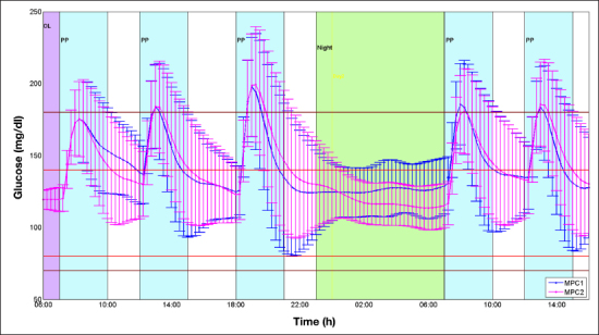
The figure shows for MPC1 (blue) and MPC2 (magenta) the mean (dots) and the variability (±standard deviation) of the glucose profiles obtained in 100 virtual patients with the sensitivity variation scenario. OL, open loop; PP, postprandial period.

Figure 6.

The figure shows for MPC1 (blue) and MPC2 (magenta) the mean (dots) and the variability (±standard deviation) of the glucose profiles obtained in 100 virtual patients with the meal variation scenario. OL, open loop; PP, postprandial period.

Figure 7.

The CVGA representing the results obtained using MPC1 (blue) and MPC2 (magenta) on the sensitivity variation scenario. Each point represents the coordinates (x is a function of the minimal glucose value and y a function of the maximal value) associated with a single patient.

The CVGA representation with the meals variation scenario (Figure 8) shows that the MPC2 doubles the number of patients in the A zone, increases those in the B zone and reduces the number of patients in the C and D zones; in particular, it was reduced by 73% in the D zone.

Figure 8.

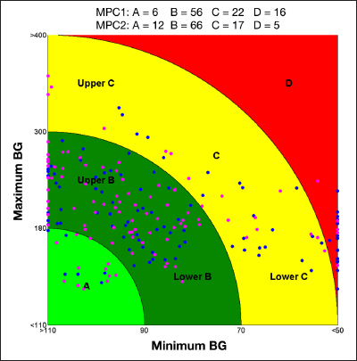
The CVGA representing the results obtained using MPC1 (blue) and MPC2 (magenta) on the meals variation scenario. Each point represents the coordinates (x is a function of the minimal glucose value and y a function of the maximal value) associated with a single patient.

Tables 5 and 6 gather the performance indexes of all algorithms for the nominal and the robustness scenarios, respectively. MPC2 lowers the mean glucose and increases the time spent in tight target in all the considered scenarios, especially during the night (p < .01); reduces the time spent below 70 mg/dl in nominal (p < .001) and meal variation (p < .01) scenarios; and always reduces the time spent below 50 mg/dl (p < .04). Moreover, the glucose standard deviations are always lowered, especially during the night (p < .003). Note that during the night, the mean glucose is almost equal to the target, and the increase of the time below 70 mg/dl in the sensitivity variation scenario is negligible (p > .78). In the meal variations scenario, as reported in Table 6, the time in target is almost 100% combined with a decrease of the time below 70 mg/dl (p < .06); a negligible increase of the mean glucose (p > .51) and the time above 180 mg/dl (p > .68) is detected in the postprandial period.

Table 5.

Results Obtained Simulating Strategies MPC1 and MPC2 on the Nominal Scenario^a

		Nominal scenario
		O	N	PP
M (mg/dl)	MPC1	140.74	124.42	156.30
	MPC2	139.57	115.96 b	157.78
	p value	0.16	8.51·10−8	0.70
SD (mg/dl)	MPC1	28.63	13.07	26.02
	MPC2	27.41	9.35b	24.55
	p value	0.20	1.28·10−5	0.10
Tt (%)	MPC1	86.33	99.02	76.22
	MPC2	87.64	99.81	77.22
	p value	0.08	0.05	0.34
Ttt (%)	MPC1	52.69	82.07	32.02
	MPC2	59.01c	94.69b	32.54
	p value	3.33·10−3	2.53·10−6	0.82
Ta ( %)	MPC1	12.45	0.78	23.18
	MPC2	12.31	0.19	22.78
	p value	0.37	0.24	0.54
Tb (%)	MPC1	1.23	0.20	0.60
	MPC2	0.05b	0.00	0.00c
	p value	4.70·10−4	0.08	1.23·10−3
Th (%)	MPC1	0.49	0.01	0.26
	MPC2	0.00c	0.00	0.00d
	p value	7.31·10−3	0.32	0.04

^aO is overall, N is night, PP is the mean relative to all postprandial periods; M is the mean of the BG (mg/dl); SD is the standard deviation of the BG (mg/dl); Tt is the percentage of time spent in euglycemic target (70–180 mg/dl); Ttt is the percentage of time spent in tight target (80–140 mg/dl); Ta is the percentage of time spent above 180 mg/dl; Tb is the percentage of time spent below 70 mg/dl; and Th is the percentage of time spent below 50 (mg/dl).

^bp < .0 01.

^cp < .01.

^dp < .05.

Table 6.

Results Obtained Simulating Strategies MPC1 and MPC2 on the Sensitivity Variation and the Meal Variation Scenarios^a

		Sensitivity variation scenario			Meals variation scenario
		O	N	PP	O	N	PP
	MPC1	143.08	125.71	158.50	139.79	124.23	157.05
M (mg/dl)	MPC2	142.38	118 . 4 9 b	160.50	140.07	116 . 0 3 b	159.66
	p value	0.82	9.08·105	0.62	0.56	1.54·10−7	0.51
	MPC1	29.90	13.03	27.08	35.87	13.34	38.35
SD	MPC2	28.63	10.29c	25.55	35.18	9.59b	37.53
	p value	0.30	2.09·10−3	0.24	0.46	6.97·10−6	0.41
	MPC1	81.75	98.66	70.02	83.89	98.92	71.74
Tt (%)	MPC2	83.06	98.68	71.71	84.54	99.66d	71.93
	p value	0.23	0.35	0.49	0.28	0.04	0.88
	MPC1	47.81	79.58	28.84	56.91	81.89	39.82
Ttt (%)	MPC2	50.65	88.55c	29.25	62.52	94.86b	40.69
	p value	0.30	9.30·103	0.91	0.01	1.63·10−6	0.76
	MPC1	15.58	1.06	27.66	13.97	0.83	26.76
Ta (%)	MPC2	15.58	0.55	27.54	14.84	0.24	27.57
	p value	0.59	0.30	0.86	0.84	0.30	0.69
	MPC1	2.69	0.30	2.31	2.12	0.25	1.49
Tb (%)	MPC2	1.38	0.78	0.74	0.61c	0.1	0.49d
	p value	0.16	0.78	0.06	1.93·10−3	0.06	0.01
	MPC1	1.27	0.00	1.25	0.76	0.01	0.62
Th (%)	MPC2	0.40d	0.09	0.23	0.12c	0	0.19
	p value	0.04	0.32	0.17	7.62·10−3	0.32	0.07

^aO is overall, N is night, PP is the mean relative to all postprandial periods; M is the mean of the BG (mg/dl); SD is the standard deviation of the BG (mg/dl); Tt is the percentage of time spent in euglycemic target (70–180 mg/dl); Ttt is the percentage of time spent in tight target (80–140 mg/dl); Ta is the percentage of time spent above 180 mg/dl; Tb is the percentage of time spent below 70 mg/dl; and Th is the percentage of time spent below 50 mg/dl.

^bp < .0 01.

^cp < .01.

^cp < .05.

Conclusions

The new MPC controller proposed in this article is an evolution of the algorithm presented by Soru and coauthors¹⁰ that was used during the CAT AP@home trial.²¹ The new MPC incorporates clinical experience included in the collected data and also some clinical knowledge that is very critical to develop an artificial pancreas ready for long-term outpatient experiments. In silico results are very promising in terms of mean glucose, time in target, and number of patients in the critical zone of the CVGA. This algorithm, complemented with the SSM,²² has been implemented on the Diabetes Assistant³⁷ and tested in an outpatient trial,³⁸ following the first outpatient studies,^39,40 which implemented a simpler hypo–hyper mitigation system always complemented with the SSM.²²

Glossary

(AP)

artificial pancreas

(BG)

blood glucose

(CAT)

Comparison of Two Artificial Pancreas Systems for Closed-Loop Blood Glucose Control versus Open-Loop Control in Patients with Type 1 Diabetes

(CGM)

continuous glucose monitoring

(CVGA)

control variability grid analysis

(LMPC)

linear model predictive control

(MPC)

model predictive control

(SC)

subcutaneous

(SSM)

safety supervision module

Funding

This work was supported by ICT FP7-247138 Bringing the Artificial Pancreas at Home (AP@home) project and the Fondo per gli Investimenti della Ricerca di Base project “Artificial Pancreas: In Silico Development and In Vivo Validation of Algorithms for Blood Glucose Control” funded by Italian Ministero dell’Istruzione, dell’Università e della Ricerca.

References

- 1.Steil GM, Rebrin K, Darwin C, Hariri F, Saad MF. Feasibility of automating insulin delivery for the treatment of type 1 diabetes. Diabetes. 2006;55(12):3344–3350. doi: 10.2337/db06-0419. [DOI] [PubMed] [Google Scholar]
- 2.Hovorka R, Canonico V, Chassin LJ, Haueter U, Massi-Benedetti M, Orsini Federici M, Pieber TR, Schaller HC, Schaupp L, Vering T, Wilinska ME. Nonlinear model predictive control of glucose concentration in subjects with type 1 diabetes. Physiol Meas. 2004;25(4):905–920. doi: 10.1088/0967-3334/25/4/010. [DOI] [PubMed] [Google Scholar]
- 3.Weinzimer SA, Steil GM, Swan KL, Dziura J, Kurtz N, Tamborlane WV. Fully automated closed-loop insulin delivery versus semiautomated hybrid control in pediatric patients with type 1 diabetes using an artificial pancreas. Diabetes Care. 2008;31(5):934–939. doi: 10.2337/dc07-1967. [DOI] [PubMed] [Google Scholar]
- 4.Hovorka R, Allen JM, Elleri D, Chassin LJ, Harris J, Xing D, Kollman C, Hovorka T, Larsen AM, Nodale M, De Palma A, Wilinska ME, Acerini CL, Dunger DB. Manual closed-loop insulin delivery in children and adolescents with type 1 diabetes: a phase 2 randomised crossover trial. Lancet. 2010;375(9716):743–751. doi: 10.1016/S0140-6736(09)61998-X. [DOI] [PubMed] [Google Scholar]
- 5.El-Khatib FH, Russell SJ, Nathan DM, Sutherlin RG, Damiano ER. A bihormonal closed-loop artificial pancreas for type 1 diabetes. Sci Transl Med. 2010;2(27):27ra27. doi: 10.1126/scitranslmed.3000619. [DOI] [PMC free article] [PubMed] [Google Scholar]
- 6.Kovatchev B, Cobelli C, Renard E, Anderson S, Breton M, Patek S, Clarke W, Bruttomesso D, Maran A, Costa S, Avogaro A, Dalla Man C, Facchinetti A, Magni L, De Nicolao G, Place J, Farret A. Multinational study of subcutaneous model-predictive closed-loop control in type 1 diabetes mellitus: summary of the results. J Diabetes Sci Technol. 2010;4(6):1374–1381. doi: 10.1177/193229681000400611. [DOI] [PMC free article] [PubMed] [Google Scholar]
- 7.Marchetti G, Barolo M, Jovanovic L, Zisser H, Seborg DE. An improved PID switching control strategy for type 1 diabetes. IEEE Trans Biomed Eng. 2008;55(3):857–865. doi: 10.1109/TBME.2008.915665. [DOI] [PubMed] [Google Scholar]
- 8.Parker RS, Doyle FJ, 3rd, Peppas NA. A model-based algorithm for blood glucose control in type I diabetic patients. IEEE Trans Biomed Eng. 1999;46(2):148–157. doi: 10.1109/10.740877. [DOI] [PubMed] [Google Scholar]
- 9.Magni L, Raimondo DM, Bossi L, Man CD, De Nicolao G, Kovatchev B, Cobelli C. Model predictive control of type 1 diabetes: an in silico trial. J Diabetes Sci Technol. 2007;1(6):804–812. doi: 10.1177/193229680700100603. [DOI] [PMC free article] [PubMed] [Google Scholar]
- 10.Soru P, De Nicolao G, Tofanin C, Dalla Man C, Cobelli C, Magni L. AP@home Consortium. MPC based Artifcial Pancreas: Strategies for individualization and meal compensation. Ann Rev Control. 2012;36(1):118–128. [Google Scholar]
- 11.Bequette BW. A critical assessment of algorithms and challenges in the development of a closed-loop artificial pancreas. Diabetes Technol Ther. 2005;7(1):28–47. doi: 10.1089/dia.2005.7.28. [DOI] [PubMed] [Google Scholar]
- 12.Hovorka R. Management of diabetes using adaptive control. Int J Adapt Control Signal Process. 2005;19(5):309–325. [Google Scholar]
- 13.Hovorka R. Continuous glucose monitoring and closed-loop systems. Diabet Med. 2006;23(1):1–12. doi: 10.1111/j.1464-5491.2005.01672.x. [DOI] [PubMed] [Google Scholar]
- 14.Grosman B, Dassau E, Zisser HC, Jovanovic L, Doyle FJ., 3rd Zone model predictive control: A strategy to minimize hyper- and hypoglycemic events. J Diabetes Sci Technol. 2010;4(4):961–975. doi: 10.1177/193229681000400428. [DOI] [PMC free article] [PubMed] [Google Scholar]
- 15.Dua P, Doyle FJ, 3rd, Pistikopoulos EN. Model-based blood glucose control for type 1 diabetes via parametric programming. IEEE Trans Biomed Eng. 2006;53(8):1478–1491. doi: 10.1109/TBME.2006.878075. [DOI] [PubMed] [Google Scholar]
- 16.Magni L, Raimondo DM, Dalla Man C, De Nicolao G, Kovatchev BP, Cobelli C. Model predictive control of glucose concentration in type I diabetic patients: an in silico trial. Biomed Signal Process Control. 2009;4(4):338–346. [Google Scholar]
- 17.Magni L, Forgione M, Tofanin C, Dalla Man C, Kovatchev B, De Nicolao G, Cobelli C. Run-to-run tuning of model predictive control for type 1 diabetes subjects: in silico trial. J Diabetes Sci Technol. 2009;3(5):1091–1098. doi: 10.1177/193229680900300512. [DOI] [PMC free article] [PubMed] [Google Scholar]
- 18.Patek SD, Magni L, Dassau E, Karvetski C, Tofanin C, De Nicolao G, Del Favero S, Breton M, Man CD, Renard E, Zisser H, Doyle FJ, 3rd, Cobelli C, Kovatchev BP. International Artifcial Pancreas (iAP) Study Group. Modular closed-loop control of diabetes. IEEE Trans Biomed Eng. 2012;59(11):2986–2999. doi: 10.1109/TBME.2012.2192930. [DOI] [PMC free article] [PubMed] [Google Scholar]
- 19.Dassau E, Zisser H, Percival M, Grosman B, Jovanovic L, Doyle FJ., 3rd Clinical results of automated artificial pancreatic beta-cell system with unannounced meal using multi-parametric MPC and insulin-on-board. Diabetes. 2010;59(1):A94. [Google Scholar]
- 20.Breton M, Farret A, Bruttomesso D, Anderson S, Magni L, Patek S, Dalla Man C, Place J, Demartini S, Del Favero S, Tofanin C, Hughes-Karvetski C, Dassau E, Zisser H, Doyle FJ, 3rd, De Nicolao G, Avogaro A, Cobelli C, Renard E, Kovatchev B. International Artifcial Pancreas Study Group. Fully integrated artificial pancreas in type 1 diabetes: modular closed-loop glucose control maintains near normoglycemia. Diabetes. 2012;61(9):2230–2237. doi: 10.2337/db11-1445. [DOI] [PMC free article] [PubMed] [Google Scholar]
- 21.Luijf YM, DeVries JH, Zwinderman K, Leelarathna L, Nodale M, Caldwell K, Kumareswaran K, Elleri D, Allen J, Wilinska M, Evans M, Hovorka R, Doll W, Ellmerer M, Mader JK, Renard E, Place J, Farret A, Cobelli C, Del Favero S, Dalla Man C, Avogaro A, Bruttomesso D, Filippi A, Scotton R, Magni L, Lanzola G, Di Palma F, Soru P, Tofanin C, De Nicolao G, Arnolds S, Benesch C, Heinemann L. AP@home Consortium. Day and night closed loop control in adults with type 1 diabetes mellitus: a comparison of two closed loop algorithms driving continuous subcutaneous insulin infusion versus patient self management. Diabetes Care. doi: 10.2337/dc12-1956. Forthcoming. [DOI] [PMC free article] [PubMed] [Google Scholar]
- 22.Hughes CS, Patek SD, Breton MD, Kovatchev BP. Hypoglycemia prevention via pump attenuation and red-yellow-green “trafc” lights using continuous glucose monitoring and insulin pump data. J Diabetes Sci Technol. 2010;4(5):1146–1155. doi: 10.1177/193229681000400513. [DOI] [PMC free article] [PubMed] [Google Scholar]
- 23.Dalla Man C, Micheletto F, Lv D, Breton M, Kovatchev BP, Cobelli C. The UVa/Padova type 1 diabetes simulator: new features. J Diabetes Sci Technol. doi: 10.1177/1932296813514502. Forthcoming. [DOI] [PMC free article] [PubMed] [Google Scholar]
- 24.Kovatchev BP, Breton MD, Dalla Man C, Cobelli C. In silico model and computer simulation environment approximating the human glucose/ insulin utilization. Food and Drug Administration Master File MAF. 2008;1521 [Google Scholar]
- 25.Breton M, Kovatchev B. Analysis, modeling, and simulation of the accuracy of continuous glucose sensors. J Diabetes Sci Technol. 2008;2(5):853–862. doi: 10.1901/jaba.2008.2-853. [DOI] [PMC free article] [PubMed] [Google Scholar]
- 26.Post TM, Freijer JI, Ploeger BA, Danhof M. Extensions to the Visual Predictive Check to facilitate model performance evaluation. J Pharmacokinet Pharmacodyn. 2008;35(2):185–202. doi: 10.1007/s10928-007-9081-1. [DOI] [PMC free article] [PubMed] [Google Scholar]
- 27.Facchinetti A, Sparacino G, Cobelli C. Modeling the error of continuous glucose monitoring sensor data: critical aspects discussed through simulation studies. J Diabetes Sci Technol. 2010;4(1):4–14. doi: 10.1177/193229681000400102. [DOI] [PMC free article] [PubMed] [Google Scholar]
- 28.Facchinetti A, Del Favero S, Sparacino G, Castle J, Ward W, Cobelli C. Modeling the glucose sensor error. IEEE Trans Biomed Eng. 2013. doi: 10.1109/TBME.2013.2284023. Epub ahead of print. [DOI] [PubMed] [Google Scholar]
- 29.Christiansen M, Bailey T, Watkins E, Liljenquist D, Price D, Nakamura K, Boock R, Peyser T. A new-generation continuous glucose monitoring system: improved accuracy and reliability compared with a previous-generation system. Diabetes Technol Ther. 2013;15(10):881–888. doi: 10.1089/dia.2013.0077. [DOI] [PMC free article] [PubMed] [Google Scholar]
- 30.Attia N, Jones TW, Holcombe J, Tamborlane WV. Comparison of human regular and lispro insulins after interruption of continuous subcutaneous insulin infusion and in the treatment of acutely decompensated IDDM. Diabetes Care. 1998;21(5):817–821. doi: 10.2337/diacare.21.5.817. [DOI] [PubMed] [Google Scholar]
- 31.Zisser H. Quantifying the impact of a short-interval interruption of insulin-pump infusion sets on glycemic excursions. Diabetes Care. 2008;31(2):238–239. doi: 10.2337/dc07-1757. [DOI] [PubMed] [Google Scholar]
- 32.Gentili M, Caltabiano D, Sannino R, Tofanin C, Di Palma F, Magni L, Lane S. Embedded implementation of modular closed-loop control of diabetes and in silico validation. Presented at 15th International Conference on e-Health Networking, Application, and Services, IEEE Healthcom’13; October 9-12, 2013; Lisbon, Portugal. [Google Scholar]
- 33.Welch BL. The generalization of “Student’s” problem when several diferent population variances are involved. Biometrika. 1947;34(1-2):28–35. doi: 10.1093/biomet/34.1-2.28. [DOI] [PubMed] [Google Scholar]
- 34.Gibbons JD. 2nd ed. New York: Marcel Dekker; 1985. Nonparametric statistical inference. [Google Scholar]
- 35.Lilliefors HW. On the Kolmogorov-Smirnov test for the exponential distribution with mean unknown. J Am Stat Assoc. 1969;64(325):387–389. [Google Scholar]
- 36.Magni L, Raimondo DM, Man CD, Breton M, Patek S, Nicolao GD, Cobelli C, Kovatchev BP. Evaluating the efficacy of closed-loop glucose regulation via control-variability grid analysis. J Diabetes Sci Technol. 2008;2(4):630–635. doi: 10.1177/193229680800200414. [DOI] [PMC free article] [PubMed] [Google Scholar]
- 37.Keith-Hynes P, Guerlain S, Mize B, Hughes-Karvetski C, Khan M, McElwee-Malloy M, Kovatchev BP. DiAs user interface: a patient-centric interface for mobile artificial pancreas systems. J Diabetes Sci Technol. 2013;7(6):1416–1426. doi: 10.1177/193229681300700602. [DOI] [PMC free article] [PubMed] [Google Scholar]
- 38.Kovatchev B, Cobelli C, Renard E, Zisser H. International Artifcial Pancreas Study Group. Efcacy of outpatient closed-loop control (CLC). Presented at the 73nd Scientifc Sessions of the American Diabetes Association; June 21-25, 2013; Chicago, IL. [Google Scholar]
- 39.Cobelli C, Renard E, Kovatchev BP, Keith-Hynes P, Ben Brahim N, Place J, Del Favero S, Breton M, Farret A, Bruttomesso D, Dassau E, Zisser H, Doyle FJ, 3rd, Patek SD, Avogaro A. Pilot Studies of wearable outpatient artificial pancreas in type 1 diabetes. Diabetes Care. 2012;35(9):e65–e67. doi: 10.2337/dc12-0660. [DOI] [PMC free article] [PubMed] [Google Scholar]
- 40.Kovatchev BP, Renard E, Cobelli C, Zisser HC, Keith-Hynes P, Anderson SM, Brown SA, Chernavvsky DR, Breton MD, Farret A, Pelletier MJ, Place J, Bruttomesso D, Del Favero S, Visentin R, Filippi A, Scotton R, Avogaro A, Doyle FJ., 3rd Feasibility of outpatient fully integrated closed-loop control: frst studies of wearable artificial pancreas. Diabetes Care. 2013;36(7):1851–1858. doi: 10.2337/dc12-1965. [DOI] [PMC free article] [PubMed] [Google Scholar]