Algorithms for a Closed-Loop Artificial Pancreas: The Case for Model Predictive Control

Abstract

The relative merits of model predictive control (MPC) and proportional-integral-derivative (PID) control are discussed, with the end goal of a closed-loop artificial pancreas (AP). It is stressed that neither MPC nor PID are single algorithms, but rather are approaches or strategies that may be implemented very differently by different engineers. The primary advantages to MPC are that (i) constraints on the insulin delivery rate (and/or insulin on board) can be explicitly included in the control calculation; (ii) it is a general framework that makes it relatively easy to include the effect of meals, exercise, and other events that are a function of the time of day; and (iii) it is flexible enough to include many different objectives, from set-point tracking (target) to zone (control to range). In the end, however, it is recognized that the control algorithm, while important, represents only a portion of the effort required to develop a closed-loop AP. Thus, any number of algorithms/approaches can be successful—the engineers involved in the design must have experience with the particular technique, including the important experience of implementing the algorithm in human studies and not simply through simulation studies.

Prelude

It is with great pleasure that I agreed to a debate with Garry Steil, Ph.D., on the relative merits of model predictive control (MPC) and proportional-integral-derivative (PID) control for use in a closed-loop artificial pancreas (AP). Dr. Steil and I have had an ongoing discussion about these two approaches during our conversations at diabetes meetings and conferences over the past decade. In a sense, we have a consensus that either approach can be used successfully in a closed-loop AP; indeed, it is hard to argue with the success that Steil and Medtronic have had in both animal and human studies using PID control, particularly with model-based insulin feedback.

In this position paper, I will first discuss how the MPC versus PID debate has occurred in other technical communities, such as chemical process control. I will then review the numerous ways of developing and implementing MPC algorithms in general. Further, I will summarize the different approaches that have been taken by research groups involved with MPC-related AP projects. Finally, I will respond explicitly to a number of points raised in Steil’s commentary.¹

Background

The so-called debate of MPC versus PID in the development of a closed-loop AP is a reincarnation of a discussion that has been ongoing in the chemical process control community since the 1990s. Indeed, for years, the perceived “gap” between academic theoreticians and industrial practitioners was lamented at numerous conferences and in journal articles. It might be natural to assume that the “gap” is due to a lack of resources or knowledge in industry to apply the advanced algorithms developed in academia, but that is not necessarily the case. Foss² proposed that academics were not developing a theoretical framework to handle the real industrial challenges. Indeed, the advanced control approach most often applied in industry is MPC, which was developed and applied by Charlie Cutler at Shell in the 1970s in the form of dynamic matrix control (DMC).³ The main attributes of the DMC approach were the ability to handle multivariable systems (more than one input and output) and to rigorously enforce constraints. Academics soon realized the importance of MPC and began developing a theoretical underpinning to the algorithms. Garcia and Morari,⁴ in a series of papers, developed the basic framework of internal model control (IMC), while Ricker⁵ developed a constrained formulation.

The notion that PID is somehow more robust than model-based control methods, which was argued for years in the process control community, has been disproved. Internal model control, which can be formulated to have the same performance as MPC, is known to be equivalent to PID under certain conditions. If a first-order model is used for IMC design, there is an equivalent proportional-integral controller; if a second-order model is used for IMC design, there is an equivalent PID controller. These examples are derived in standard undergraduate textbooks,⁶ as noted in my review article,⁷ and, with the AP in mind, in the work of Percival and coauthors.⁸ Higher-order models can result in controllers that are similar to PID but with additional elements, such as lead lag or explicit time-delay compensation. A take-home message from this background is that model-based controllers that are designed to meet the same performance criteria as PID controllers will also have the same degree of robustness (sensitivity to uncertainty).

It has also been argued that model-based controllers are much more complex to implement than PID. Pannocchia and coauthors⁹ outlined six myths regarding PID control and showed that a constrained linear-quadratic-based algorithm had better performance for both set-point changes and disturbance rejection, with little additional computational time. It should further be noted that industrial PID controllers often have far more than the three standard tuning parameters (proportional, integral, and derivative) that must be specified, including absolute and rate limits, antireset windup features, selection of error or process output for derivative action, and derivative filter, among numerous others (that are most often left at factory default settings).

I should also note that there is a tendency to think of the control algorithm as the major part of the closed-loop strategy. In reality, the specific algorithm that takes a measured signal and determines the next manipulated input change is a relatively small, albeit important, part of the closed-loop system. It is important to have various levels of signal verification, fault detection, and safety checks and to have reliable hardware components (sensor and pump) and a user-friendly interface so that the “operator” (who is also the “plant/process” part of the closed-loop AP system, in our case) can easily monitor system performance and respond to alarms and fault conditions. For an overview of challenges related to a closed-loop AP, see my previous publication.¹⁰

Model Predictive Control

Model predictive control is not a single algorithm, but rather a general approach. The basic principles are that a model is used to predict the effect of control moves on future outputs, and an optimization is performed to select the best set of current and control moves to satisfy an objective. The basic idea is shown in Figure 1 for a constant future set point.

Figure 1.

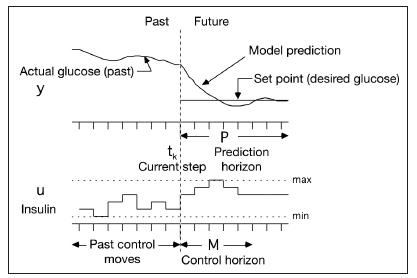
Basic concept of MPC. At the current time step, a model is used to predict the effect of proposed current and future manipulated input (insulin infusion) changes on the desired output (glucose) over a prediction horizon. Minimum and maximum (constraints) infusion rates can be enforced. Notice that the prediction horizon is often larger than the control horizon. P, prediction horizon; M, control horizon.

Here we discuss the following important topics when implementing MPC: (i) type of model, (ii) correcting process– model mismatch, (iii) control objective, and (iv) optimization/solution method. Qin and Badgwell¹¹ present a nice survey of industrial applications that reviews these various topics from a chemical process control perspective.

Type of Model

Mathematical models of many forms can be used. A natural formulation consists of continuous ordinary diferential equations, which can be linear or nonlinear; often, compartmental-based models are formulated. Analytical solutions can be used for linear equations, while nonlinear equations are integrated numerically. More often, discrete-time models are used, with any number of forms. Linear discrete models can be in the form of state space, autoregressive moving average with exogenous input (ARX), or step response. A model in any of these forms can be transformed to any of the other forms using standard techniques. Discrete nonlinear models, such as those developed based on artificial neural networks, can also be used. The mathematical model is used to predict the effect of proposed control moves on future states and outputs. It is necessary then at each time step to integrate or solve the equations based on state values at that time step. How this is performed is related to the next topic.

Correcting for Plant–Model Mismatch

Since no model is perfect, it is important to correct or update the model based on measurements. The simplest approach, used in the original DMC formulation, is simply to calculate the difference between the measured output and the model prediction at the current time step and assume that this constant difference holds in the future predictions; this is the additive output disturbance assumption. When this approach is used, uncompensated model predictions are simply obtained by continuing to integrate the model equations from step to step without changing the states based on the new measurements. The only model correction is then applied to the predicted output; not the states. An alternative approach is to use an appended state Kalman filter or other type of state observer method. Indeed, improved disturbance rejection can be improved using these techniques, resulting in two-degrees-of-freedom design. It should be noted that very few MPC AP papers actual discuss how the plant–model mismatch is corrected, so in most cases, it is likely to be the additive output disturbance assumption.

Objective Function

A major advantage to MPC is that any type of objective function can be used. The most common is to minimize a quadratic function (least squares) of the differences between the desired set point and model predictions (glucose) over the prediction time horizon. It is also normal to include a penalty on the control moves (changes in insulin infusion rate) over that horizon. An alternative to controlling to a desired set point is maintaining the outputs between desired high and low values (this is commonly called control to range); values predicted to be outside this range are penalized. While these bounds are usually constant at, say, 80 and 150 mg/dl, a “funnel” could be used where the target zone gets smaller further into the future.

Also, while it is common to use a prediction horizon that includes all points within that horizon, some control strategies consider a subset of the points. A coincidence point strategy, for example, would seek to minimize the control move effort (changes in insulin delivery) while satisfying a desired set point at the end of the prediction horizon.

Another major advantage of MPC is that the objective can include more than blood glucose and insulin infusion rates. The optimization formulation can include insulin on board, most often in the form of constraints (allowing a maximum insulin on board at any point over the prediction horizon). This is particularly important because the calculated current and future insulin inputs continue to have a pharmacodynamic effect 6–8 h in the future. Further, the objective can be to minimize asymmetric risk measures that recognize that a -50 mg/dl deviation is much more undesirable than a +50 mg/dl deviation from set point.

Optimization Method

A number of optimization methods can be used, depending on the form of the model and the objective function. A linear model and a quadratic objective function without constraints has an analytical (closed-form) solution. When there are constraints, a quadratic program results,¹² and there are efficient numerical methods for obtaining a solution.

Whether linear or nonlinear models are used, it is convenient to separate the model predictions into two contributions: free and forced response. Free response is the future glucose concentration that would result if no further changes were made to insulin infusion rate. Forced response is the additional contribution of insulin infusion rate changes; optimization is performed based on the forced response behavior.

Because the solution of a constrained optimization problem is iterative, there is the potential for a long computation time, which could also drain the battery on computational devices. An alternative is to use multiparametric programming, which reduces the online computation to a table look-up formulation, dramatically reducing the computational resources needed.

Models: Fixed versus Adaptive

Controllers, whether MPC or PID, can be fixed (parameters are kept constant for a particular individual) or adaptive. Typically, the parameters of a low-order discrete model are updated in real time, and the resulting updated model is used as the basis for the control calculation, whether MPC or PID is used. A major challenge with adaptive control is that it is possible for the estimated parameters to result in a model that is inconsistent with what is known physically about the system—for example, the parameters may result in an open-loop unstable system when the system is known to be open-loop stable. It is important, then, to perform additional checks to force the updated model to be stable.

Note that controllers that are tuned differently depending on the time of day, for example, are not considered adaptive because the parameters remain fixed during that time period.

Tuning Model Predictive Control

There are a substantial number of control-related tuning parameters that can be adjusted to change the closed-loop performance. The prediction and control horizons and weights on the manipulated inputs are commonly used. When a Kalman filter is used to provide model updates, the input-to-measurement-noise ratio is often used as a tuning parameter. The closed-loop performance is also affected by set point filtering, where the future set point changes from the current measured output to the desired constant set point over a number of time steps.

Model-Predictive-Control-Based Closed-Loop Artificial Pancreas Studies

With the background provided earlier, I now wish to review the MPC strategies used by groups developing a closed-loop AP. I should note that the algorithms are often presented in more detail in the initial simulation-based studies, but it is not always clear how these algorithms are modified for clinical studies. Note also that I will not review early approaches that were based solely on simulation studies assuming intravenous insulin delivery and direct blood glucose sampling. In this article, I will focus on studies involving subcutaneous insulin delivery and continuous glucose monitoring (CGM, although in a few cases these values are mimicked by simply delaying available blood glucose samples). Where possible, we will discuss model type, sample time, objective function, prediction and control horizons, plant–model mismatch compensation, and set point (including reference trajectory).

Cambridge (Hovorka)

Hovorka and coauthors¹³ developed a nonlinear compartmental model with nine parameters that are constant for all subjects and six parameters that are estimated and updated in real time; Bayesian techniques and varying window lengths of past data are used to update parameter values that best match the model predictions to the actual glucose measurements. The nonlinearity enters as the effect of insulin concentration on endogenous glucose production and transfer between accessible and nonaccessible compartments. The nonlinear compartmental model was used as the basis for a nonlinear MPC strategy that was applied in 15 overnight studies of 8–10 h duration. The sample time was 15 min, with intravenous glucose measurements delayed by 30 min to simulate CGM sensor and physiological lag. The prediction horizon was 4 h, and a maximum insulin infusion rate of 4 U/h was applied. Different reference set point trajectories were used, depending on whether the subject was above or below the set point. Hovorka and coauthors¹⁴ provide further background on the project, the role of simulation studies conducted before the clinical studies, and additional clinical studies.

Elleri and coauthors¹⁵ revised the parameter estimation procedure from Hovorka and coauthors.^{13, 14} Two model parameters are updated in real time: an endogenous glucose flux adjusting for errors in model-based predictions and carbohydrate bioavailability. Several models differing in the rate of subcutaneous insulin absorption and the carbohydrate absorption profile are run in parallel. A combined model forecasts plasma glucose excursions over a 2.5 h prediction horizon. Insulin infusion is calculated to achieve target glucose, which is set at 104 mg/dl, but it is flexible and may increase to up to 131 mg/dl if prior model predictions are less accurate. Safety rules can reduce insulin infusion.

Elleri and coauthors¹⁶ performed 36 h studies in adolescents. The algorithm is similar to the previous algorithm by Elleri and coauthors¹⁵ and is initialized using the subject’s weight, total daily dose (TDD) of insulin (mean of the previous 3 days), and the 24 h basal insulin profile programmed on the pump. The algorithm is adapted by updating endogenous glucose flux and carbohydrate bioavailability.

Hovorka and coauthors¹⁷ also used a sample time of 15 min. A nurse took a glucose reading, the controller performed the calculation, and the nurse entered the insulin pump rate manually. The algorithm was initialized using the participant’s weight, TDD of insulin, and basal insulin requirements. The algorithm was provided with sensor glucose levels during a 30 min period before the start of closed-loop delivery, the carbohydrates in the evening meal, and the prandial insulin bolus. The algorithm aims to achieve glucose levels between 104 and 131 mg/dl and adjusts the actual level depending on fasting versus postprandial status, preceding glucose levels, and the accuracy of predictions. Safety rules limit the maximum insulin infusion and suspend insulin delivery when the sensor-measured glucose is at or below 77 mg/dl or when the sensor detects that glucose is decreasing rapidly.

Virginia–Padova (Magni, Kovatchev, Cobelli)

Magni and coauthors¹⁸ linearized a nonlinear compartmental model around the basal conditions. An analytical solution to the unconstrained optimization problem was used. A 15 min sample time was used, with a prediction horizon of eight steps (120 min), control horizon of seven moves (105 min), and control weight of q = 0.003; the se t point was 112 mg/dl. There was a direct comparison with a PID controller. Bruttomesso and coauthors¹⁹ revised the Magni and coauthors¹⁸ approach, using a 240 min prediction horizon and 225 min control horizon. Six subjects were studied in 22 h overnight sessions. The algorithm used glucose and insulin infusion information from the previous 45 min.

Kovatchev and coauthors²⁰ conducted a multicenter trial (22 h, 14.5 h closed-loop) with 20 adult subjects based on simulation studies of 300 subjects. A 1 min sensor sample time and 15 min infusion sample time were used. The algorithm was initialized with subject weight, TDD, basal, and carbohydrate-to-insulin ratio (CIR). The tuning parameter, q, was held constant (not given). The controller calculated the infusion rate, which was then entered manually. Clarke and coauthors²¹ studied eight subjects overnight and 4 h after a meal. The algorithm was initialized using a three-parameter log linear regression based on weight (kilograms), average TDD of insulin, and blood glucose correction factor measured during the first admission.

Soru and coauthors²² discussed techniques for meal compensation and individualization for better performance in simulation studies involving four different scenarios and 100 subjects. They first used a single adjustable parameter based on clinical parameters (MPC1). They then developed low-order models to produce a more realistic model as a basis for MPC; this model was further revised based on patient-specific information (MPC2).

University of California, Santa Barbara/Sansum (Doyle)

Doyle and coauthors^23–25 used two separate approaches—one based on zone MPC and the other based on parametric programming MPC. In both approaches, a discrete ARX model individualized with subject-specific tuning parameters is used. The sample time is 5 min. A control-to-range-type approach, known as zone MPC, was used in simulation studies by Grosman and coauthors;²³ prediction and control horizons of 180 and 25 min, respectively, were used. Dassau and coauthors²⁴ presented clinical results using a multiparametric MPC algorithm, which has the advantage of a fast computation time; 6 h prediction and 30 min control horizons were used. Simulation results are presented were Percival and coauthors.²⁵

Boston/Massachusetts General Hospital (Damiano)

El-Khatib and coauthors^26,27 used a generalized predictive control (GPC) formulation based on low-order ARX models and using short prediction and control horizons (one step each), resulting in a low-order controller similar to PID. The model parameters are adapted in real time; a challenge to this approach is that it is possible for the control law to be unstable if a nonminimum phase model is estimated. To assure stability for a one-step-ahead controller, a large penalty must be applied to the manipulated input action. The main strength of the method is that the plasma insulin concentration is explicitly calculated and used in the objective function, thus the effect of previous insulin infusions is considered. Glucagon is also manipulated using a proportional-derivative controller.

Illinois Institute of Technology (Cinar)

Cinar and coauthors^28,29 also used an adaptive GPC strategy. Their method ensures that the estimated parameters result in a stable model. Turksoy and coauthors²⁹ used a 10 min sample time, with prediction and control horizons of 8 (80 min) and 6 (60 min), respectively, and included activity signals from a SenseWear armband. The insulin infusion rate computed by the algorithm was entered manually. The set point was 120 mg/dl, with a fast set point trajectory if below this value and a slower trajectory if above this value.

Rensselaer/Stanford (Bequette)

Lee and coauthors^30,31 used subspace identification techniques to develop discrete state space models and incorporate insulin-on-board constraints in MPC; additional features include a pump shut-off algorithm to avoid hypoglycemia and meal detection and meal size estimation algorithms to handle unannounced meals. A sample time of 5 min was used, with prediction and control horizons of 120 and 25 min, respectively.

Cameron and coauthors³² developed a multiple model probabilistic predictive control (MMPPC) approach, with meal probabilities continuously estimated to detect unannounced meals; extensions to the meal modeling approach are presented by Cameron and coauthors.³³ In simulation studies, a risk measure is minimized, also considering the uncertainty (using a probability distribution). A discrete compartmental model is used, which is individualized by a correction factor based on TDD, using the 1800 rule. The prediction horizon is 300 min, with a control horizon of one move. The performance of the MMPPC strategy is compared with several other algorithms in Figure 2 (where EMPC refers to the MMPPC strategy). Cameron and coauthors³⁴ revised the approach used in simulation studies for their clinical studies involving 10 subjects. The probability-based approach is now used to select an insulin bolus that gives a 3% risk of blood glucose going below 80 mg/dl during the prediction horizon of 300 min.

Figure 2.

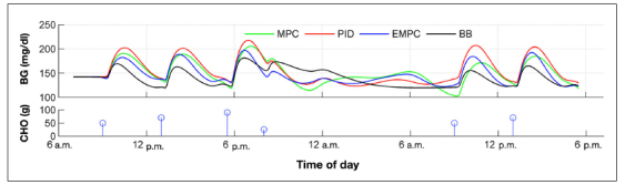
Performance of controllers averaged over the nine valid simulated subjects. Enhanced MPC is the MMPPC strategy. The PID controller parameters were adjusted to minimize the blood glucose risk index averaged over the subjects. The MPC represents a “standard” MPC strategy with a symmetric objective function. The basal–bolus strategy represents optimal performance and is based on perfect meal knowledge; none of the other strategies used meal anticipation. Figure reproduced with permission from Cameron and coauthors.³² CHO, carbohydrate; BG, blood glucose; EMPC, enhanced model predictive control; BB, basal–bolus.

Summary of Model Predictive Control Artificial Pancreas Strategies

The only clinical study to date comparing different MPC algorithms was reported by De Vries and coauthors.³⁵ The MPC1 algorithm of Soru and coauthors²² and the MPC algorithm of Hovorka and coauthors³⁶ were studied in trials involving 47 patients in six centers; while the closed-loop algorithms each had a higher mean glucose than open-loop control, both resulted in less time in hypoglycemia than open-loop control.

The MPC studies reviewed in this paper are summarized in Table 1 . Clearly there are many different implementations by the various research groups. Indeed, most groups have applied more than one MPC technique, and algorithms have generally been modified between the simulation and clinical studies.

Table 1.

Summary of Model Predictive Control Approaches Used in the Closed-Loop Artificial Pancreas

First author	Model type	Model initialization	Objective function	Prediction and control horizons	Sample time	Model error comp	Set point	Notes
Hovorka13, 14	Nonlinear compartmental		Quadratic	240 min	15 min	Bayesian estimation of six parameters; three learning window horizons are used	108 mg/dl; filtered, faster from below, slower from above	Max 4 U/h
Elleri,15, 16 Hovorka17	Compartmental model	Weight, TDD, basal profile	Quadratic	150 min (prediction)	15 min	Endogenous glucose production and carbohydrate bioavailability are adjusted	104 mg/dl; higher when model is less certain
Magni18	Linearized compartmental model, reduced	Average population values	Quadratic, unconstrained (analytical)	120 min (prediction), 105 min (control)	15 min	Not discussed	112 mg/dl	Simulation studies; comparison with PID; q parameter used for tuning; meal announcement
Bruttomesso19	Linearized compartmental model, reduced	Weight, TDD, CIR, premeal glucose, insulin concentration, all used to set the q tuning parameter	Quadratic, unconstrained (analytical)	240 min (prediction), 225 min (control)	15 min (1 min CGM)	Not discussed	112 mg/dl	Six clinical subjects, 22 h overnight hospital
Kovatchev20	Linearized compartmental model, reduced	Weight, TDD, CIR, q (control weight)	Quadratic, unconstrained (analytical)	240 min (prediction), 225 min (control)	15 min (1 min CGM)	Not discussed	112 mg/dl	300 simulated subjects, 20 clinical subjects
Clarke21	Linearized compartmental model, reduced	3-parameter log regression based on weight, TDD, correction factor	Quadratic, unconstrained (analytical)		15 min (1 min CGM)		112 mg/dl	8 clinical subjects
Soru22	Linear state space	MPC1: linear, average subject model; MPC2: individually estimated models	Quadratic, unconstrained (analytical)	600 min	Not discussed, probably 15 min with 1 min CGM	Kalman filter	110 mg/dl	Simulation studies
Percival25 (simulation), Dassau24 (clinical)	Linear, low-order transfer function (discretized and implemented with state space)	Clinical parameters: correction factor, CIR	Quadratic, uses multiparametric programming	6 h (prediction), 30 min (control)	5 min	Additive output	110 mg/dl	Simulations using Hovorka and University of Virginia simulators; clinical trials, 18 fully closed-loop sessions
Grosman23	Linear ARX	Individual model fit to open-loop data based on specific test protocols; parameters constrained to assure realistic behavior	Zone with quadratic penalties outside zone; minimum of control moves over control horizon	180 min (prediction), 25 min (control)	5 min	Details of state updates not discussed	Zone (between minimum and maximum glucose values)	10 simulated subjects; 9 simulated experiments; uses "mapped input" values based on second-order transfer functions
El-Khatib26, 27	Linear, adaptive, second-order ARX	Subject weight	Quadratic	5 min (prediction and control)	5 min	Parameter estimates		GPC form, glucagon via PID
Eren-Oruklu,28Turksoy29	Linear, adaptive, ARX	Individual model, parameters estimated in real time	Quadratic	80 min (prediction), 60 min (control)	10 min	Parameter estimates, model constrained to assure stability	120 mg/dl; filtered, faster from below, slower from above	GPC, multivariable, includes activity monitor
Lee30–31	Linear, discrete state space	Human-friendly identification	Quadratic, with constraints (quadratic program solution)	120 min (prediction), 25 min (control)	5 min	Additive output plus meal size estimate	100 mg/dl	Output constraints are also applied; simulation studies only
Cameron32	Linear compartmental, multiple meal	Weight, TDD	Risk measure	300 min	5 min	Multiple model weighting	Minimal risk occurs at roughly 140 mg/dl	Simulation studies; a comparison with PID and the MPC method of Magni and coauthors18 is provided
Cameron34	Linear compartmental, multiple meal	Weight, TDD	Probability of glucose violating a hypoglycémie threshold	300 min	5 min	Multiple model weighting	Satisfy specified risk of glucose below 80 mg/dl	Clinical, 10 subjects, different tuning for night versus day

Proportional-Integral-Derivative Control

Similar to MPC, there is no single PID algorithm. A PID-type algorithm can be designed, tuned, and implemented in a large number of ways. Most undergraduate process control textbooks spend more than one chapter developing and expanding on the various techniques. It should also be noted that different fields of control express even the ideal form of the PID algorithm in different ways. The most common representation in the chemical process control community is

$$\begin{array}{c}e\left(t\right)=r\left(t\right)-y\left(t\right)\\ u\left(t\right)=u_0+k_c\left[e\right(t)+\frac{1}{{\tau }_1}{\int }_0^{t}e\left(t\right)dt+{\tau }_D\frac{de\left(t\right)}{d\left(t\right)}],\end{array}$$ (1)

while other disciplines often use the form

$$u(t)=u0+P\cdot e(t)+I{\displaystyle {\int }_0^{t}e(t)dt+D\cdot \frac{de}{dt}.}$$ (2)

The tuning parameter values in these two forms are related by

$$P=k_{c,}I=\frac{k_c}{{\tau }_I},D=k_c\cdot {\tau }_D,$$ (3)

which is seemingly straightforward, but the result is that one needs to be careful when performing controller tuning. Tweaking the proportional gain (k_c) while keeping the integral and derivative times constant in the first implementation requires that all three parameters (proportional, integral, and derivative) be tweaked in the second implementation. So, simply adjusting the controller gain in the first implementation is straightforward but must be coordinated with changing the integral and derivative constants in the second implementation. Further, the ideal equations presented here assume a continuous-time implementation, while in practice, the PID algorithms are implemented in discrete time (using a digital device); there are many ways to convert the continuous-time equations to discrete time. In addition, there are digital filters that must be tuned, the derivative is often taken on the measured output rather than the error, and there are different derivative approximations. Also, as noted earlier, commercial PID controllers have many additional terms to specify, such as rate limits. Finally, there are many different ways of tuning a PID controller; indeed, most undergraduate control textbooks have multiple chapters related to tuning PID controllers.

Response to Issues Raised by Steil

Dr. Steil raises some very good points in his article. For one, there is no question that a model-based controller must be based on a different model than that used by the simulator. At a minimum, the parameters used by the model in the controller must be different than the parameter values used by the simulator; this is known as parametric uncertainty. Also, the simulator model should have a higher degree of complexity, usually in the form of more equations, than the model used by the controller; this is model structure uncertainty. Most of the simulation-based studies that I have cited have both parametric and structure uncertainty.

I also agree that it is very difficult, even in simulation studies, to have a valid comparison of different algorithms. One way or another, an algorithm must be tuned based on some performance criterion, so if particular MPC and PID algorithms are tuned with different criteria, then there is no good way to compare them. Perhaps the best way to conduct a detailed simulation-based study, for example, would be to have a common basis for judgment of performance. It would probably be best to use metrics that are preferred by clinicians, such as time in range as well as times below hypoglycemic and above hyperglycemic thresholds; note that, by nature, these are multiobjective metrics.

Finally, I need to reiterate that MPC is not inherently any more sensitive to model uncertainty than PID control. While PID is not necessarily explicitly designed based on a model, the set of controller tuning parameters can be considered equivalent to a model-based controller based on a nominal model. If a controller is designed for “tight performance” based on a nominal model, it will inevitably have poor performance under realistic changes in the process behavior—this is true whether MPC or PID control is implemented.

Conclusions

I advocate MPC because of the flexible framework and the ability to explicitly incorporate constraints. Model predictive control also provides a more general framework for considering the effect of additional inputs and/or disturbances. For example, activity information can be used to predict the effect of exercise on blood glucose.

The control algorithm, however, is only one component in the closed-loop system. It is extremely important that the system be properly integrated, with reliable sensors and pumps and an easy-to-use interface. Patient safety is naturally an overriding concern, so any system must have appropriate overrides in the event of anomalous signals. Thus, while I am a strong proponent of MPC, I recognize that other algorithms/approaches, such as PID and fuzzy logic can be successfully incorporated into a closed-loop AP.

Glossary

(AP)

artificial pancreas

(ARX)

autoregressive moving average

(CGM)

continuous glucose monitoring

(CIR)

carbohydrate-to-insulin ratio

(DMC)

dynamic matrix control

(GPC)

generalized predictive control

(MPC)

model predictive control

(MMPPC)

multiple model probabilistic predictive control

(PID)

proportional integral derivative

(TDD)

total daily dose

Funding

This work was supported in part by the JDRF Grants 22–2011–647, 22–2009–795, and 22–2007–1801, and the National Institutes of Health, 5R01DK085591–03.

References

- 1.Steil GM. Algorithms for a closed-loop artificial pancreas: the case for proportional-integral-derivative control. J Diabetes Sci Technol. 2013;7(6):1632–1643. doi: 10.1177/193229681300700623. [DOI] [PMC free article] [PubMed] [Google Scholar]
- 2.Foss AS. Critique of chemical process control theory. AIChE J. 1973;19(2):209–214. [Google Scholar]
- 3.Cutler CR, Ramaker BL. Dynamic matrix control: a computer control algorithm. Proceedings of the Joint Automatic Control Conference; San Francisco, CA. 1980. paper WP5-B. [Google Scholar]
- 4.Garcia CE, Morari M. Internal model control. A unifying review and some new results. Ind Eng Chem Proc Des Dev. 1982;21(2):308–323. [Google Scholar]
- 5.Ricker NL. Use of quadratic programming for constrained internal model control. Ind Eng Chem Proc Des Dev. 1985;24(4):925–936. [Google Scholar]
- 6.Bequette BW. Upper Saddle River: Prentice Hall; 2003. Process control: modeling, design and simulation. [Google Scholar]
- 7.Bequette BW. A critical assessment of algorithms and challenges in the development of a closed-loop artificial pancreas. Diabetes Technol Ther. 2005;7(1):28–47. doi: 10.1089/dia.2005.7.28. [DOI] [PubMed] [Google Scholar]
- 8.ercival MW, Zisser H, Jovanovic L, Doyle FJ. Closed-loop control and advisory mode evaluation of an artificial pancreatic beta cell: use of proportional-integral-derivative equivalent model-based controllers. J Diabetes Sci Technol. (3rd) 2008;2(4):636–644. doi: 10.1177/193229680800200415. [DOI] [PMC free article] [PubMed] [Google Scholar]
- 9.Pannocchia G, Laachi N, Rawlings JB. A candidate to replace PID control: SISO-Constrained LQ control. AIChE J. 2005;51(4):1178–1189. [Google Scholar]
- 10.Bequette BW. Challenges and recent progress in the development of a closed-loop artificial pancreas. Annu Rev Control. 2012;36(2):255–266. doi: 10.1016/j.arcontrol.2012.09.007. [DOI] [PMC free article] [PubMed] [Google Scholar]
- 11.Qin SJ, Badgwell TA. A survey of industrial model predictive control technology. Cont Eng Pract. 2003;11:733–764. [Google Scholar]
- 12.Garcia CE, Morshedi AM. Quadratic programming solution of dynamic matrix control (QDMC) Chem Eng Commun. 1986;46:73–87. [Google Scholar]
- 13.Hovorka R, Canonico V, Chassin LJ, Haueter U, Massi-Benedetti M, Orsini Federici M, Pieber TR, Schaller HC, Schaupp L, Vering T, Wilinska ME. Nonlinear model predictive control of glucose concentration in subjects with type 1 diabetes. Physiol Meas. 2004;25(4):905–920. doi: 10.1088/0967-3334/25/4/010. [DOI] [PubMed] [Google Scholar]
- 14.Hovorka R, Chassin LJ, Wilinska ME, Canonico V, Akwi JA, Federici MO, Massi-Benedetti M, Hutzli I, Zaugg C, Kaufmann H, Both M, Vering T, Schaller HC, Schaupp L, Bodenlenz M, Pieber TR. Closing the loop: the Adicol experience. Diabetes Technol Ther. 2004;6(3):307–318. doi: 10.1089/152091504774197990. [DOI] [PubMed] [Google Scholar]
- 15.Elleri D, Allen JM, Nodale M, Wilinska ME, Mangat JS, Larsen AM, Acerini CL, Dunger DB, Hovorka R. Automated overnight closed-loop glucose control in young children with type 1 diabetes. Diabetes Technol Ther. 2011;13(4):419–424. doi: 10.1089/dia.2010.0176. [DOI] [PubMed] [Google Scholar]
- 16.Elleri D, Allen JM, Kumareswaran K, Leelarathna L, Nodale M, Caldwell K, Cheng P, Kollman C, Haidar A, Murphy HR, Wilinska ME, Acerini CL, Dunger DB, Hovorka R. Closed-loop basal insulin delivery over 36 hours in adolescents with type 1 diabetes. Diabetes Care. 2013;36(4):838–844. doi: 10.2337/dc12-0816. [DOI] [PMC free article] [PubMed] [Google Scholar]
- 17.Hovorka R, Nodale M, Haidar A, Wilinska M. Assessing performance of closed-loop insulin delivery systems by continuous glucose monitoring: drawbacks and way forward. Diabetes Technol Ther. 2013;15(1):4–12. doi: 10.1089/dia.2012.0185. [DOI] [PMC free article] [PubMed] [Google Scholar]
- 18.Magni L, Raimondo DM, Bossi L, Man CD, De Nicolao G, Kovatchev B, Cobelli C. Model predictive control of type 1 diabetes: an in silico trial. J Diabetes Sci Technol. 2007;1(6):804–812. doi: 10.1177/193229680700100603. [DOI] [PMC free article] [PubMed] [Google Scholar]
- 19.Bruttomesso D, Farret A, Costa S, Marescotti MC, Vettore M, Avogaro A, Tiengo A, Dalla Man C, Place J, Facchinetti A, Guerra S, Magni L, De Nicolao G, Cobelli C, Renard E, Maran A. Closed-loop artificial pancreas using subcutaneous glucose sensing and insulin delivery and a model predictive control algorithm: preliminary studies in Padova and Montpellier. J Diabetes Sci Technol. 2009;3(5):1014–1021. doi: 10.1177/193229680900300504. [DOI] [PMC free article] [PubMed] [Google Scholar]
- 20.Kovatchev B, Cobelli C, Renard E, Anderson S, Breton M, Patek S, Clarke W, Bruttomesso D, Maran A, Costa S, Avogaro A, Dalla Man C, Facchinetti A, Magni L, De Nicolao G, Place J, Farret A. Multinational study of subcutaneous model-predictive closed-loop control in type 1 diabetes mellitus: summary of the results. J Diabetes Sci Technol. 2010;4(6):1374–1381. doi: 10.1177/193229681000400611. [DOI] [PMC free article] [PubMed] [Google Scholar]
- 21.Clarke WL, Anderson S, Breton M, Patek S, Kashmer L, Kovatchev B. Closed-loop artificial pancreas using subcutaneous glucose sensing and insulin delivery and a model predictive control algorithm: the Virginia experience. J Diabetes Sci Technol. 2009;3(5):1031–1038. doi: 10.1177/193229680900300506. [DOI] [PMC free article] [PubMed] [Google Scholar]
- 22.Soru P, De Nicolao G, Tofanin C, Dalla Man C, Cobelli C, Magni L. MPC based Artificial Pancreas: strategies for individualization and meal compensation. Ann Rev Control. 2012;36:118–128. [Google Scholar]
- 23.Grosman B, Dassau E, Zisser HC, Jovanovic L, Doyle FJ. Zone model predictive control: A strategy to minimize hyper- and hypoglycemic events. J Diabetes Sci Technol. (3rd) 2010;4(4):961–975. doi: 10.1177/193229681000400428. [DOI] [PMC free article] [PubMed] [Google Scholar]
- 24.Dassau E, Zisser H, Harvey RA, Percival MW, Grosman B, Bevier W, Atlas E, Miller S, Nimri R, Jovanovic L, Doyle FJ. Clinical evaluation of a personalized artificial pancreas. Diabetes Care. (3rd) 2013;36(4):801–809. doi: 10.2337/dc12-0948. [DOI] [PMC free article] [PubMed] [Google Scholar]
- 25.Percival MW, Wang Y, Grosman B, Dassau E, Zisser H, Jovanovič L, Doyle FJ. Development of a multi-parametric model predictive control algorithm for insulin delivery in type 1 diabetes mellitus using clinical parameters. J Process Control. (3rd) 2011;21(3):391–404. doi: 10.1016/j.jprocont.2010.10.003. [DOI] [PMC free article] [PubMed] [Google Scholar]
- 26.El-Khatib FH, Jiang J, Damiano ER. Adaptive closed-loop control provides blood-glucose regulation using dual subcutaneous insulin and glucagon infusion in diabetic swine. J Diabetes Sci Technol. 2007;1(2):181–192. doi: 10.1177/193229680700100208. [DOI] [PMC free article] [PubMed] [Google Scholar]
- 27.El-Khatib FH, Russell SJ, Nathan DM, Sutherlin RG, Damiano ER. A bihormonal closed-loop artificial pancreas for type 1 diabetes. Sci Transl Med. 2010;2(27):27ra27. doi: 10.1126/scitranslmed.3000619. [DOI] [PMC free article] [PubMed] [Google Scholar]
- 28.Eren-Oruklu M, Cinar A, Quinn L, Smith D. Adaptive control strategy for regulation of blood glucose levels in patients with type 1 diabetes. J Proc Cont. 2009;19(8):1333–1346. [Google Scholar]
- 29.Turksoy K, Bayrak ES, Quinn L, Littlejohn E, Cinar A. Multivariable adaptive closed-loop control of an artificial pancreas without meal and activity announcement. Diabetes Technol Ther. 2013;15(5):386–400. doi: 10.1089/dia.2012.0283. [DOI] [PMC free article] [PubMed] [Google Scholar]
- 30.Lee H, Buckingham BA, Wilson DM, Bequette BW. A closed-loop artificial pancreas using model predictive control and a sliding meal size estimator. J Diabetes Sci Technol. 2009;3(5):1082–1090. doi: 10.1177/193229680900300511. [DOI] [PMC free article] [PubMed] [Google Scholar]
- 31.Lee H, Bequette BW. A closed-loop artificial pancreas based on MPC: human-friendly identification and automatic meal disturbance rejection. Biomed Signal Process Cont. 2009;4(4):347–354. [Google Scholar]
- 32.Cameron F, Bequette BW, Wilson DM, Buckingham BA, Lee H, Niemeyer G. Closed-loop artificial pancreas based on risk management. J Diabetes Sci Technol. 2011;5(2):368–379. doi: 10.1177/193229681100500226. [DOI] [PMC free article] [PubMed] [Google Scholar]
- 33.Cameron F, Niemeyer G, Bequette BW. Extended multiple model prediction with application to blood glucose regulation. J Proc Cont. 2012;12(7):1422–1432. [Google Scholar]
- 34.Cameron F, Niemeyer G, Wilson DM, Benasi K, Clinton P, Bequette BW, Buckingham BA. Clinical trials of a closed-loop artificial pancreas with large unannounced meals. American Diabetes Association Annual Meeting; Chicago, IL. 2013. Jun, [Google Scholar]
- 35.De Vries JH, Avogaro A, Benesch C, Bruttomesso D, Caldwell K, Cobelli C, Doll W, Del Favero S, Heinemann L, Hovorka R, Leelarathna L, Luijf YM, Mader J, Magni L, Nodale M, Place J, Renard E, Tofanin C. AP@HOME CONSORTIUM: Comparison of two closed loop algorithms with open loop control in type 1 diabetes. American Diabetes Association, 72nd Scientifc Sessions; Philadelphia, PA. 2012. [DOI] [PMC free article] [PubMed] [Google Scholar]
- 36.Hovorka R, Allen JM, Elleri D, Chassin LJ, Harris J, Xing D, Kollman C, Hovorka T, Larsen AM, Nodale M, De Palma A, Wilinska ME, Acerini CL, Dunger DB. 9716. Vol. 375. Lancet: 2010. Manual closed-loop insulin delivery in children and adolescents with type 1 diabetes: a phase 2 randomised crossover trial; pp. 743–751. [DOI] [PubMed] [Google Scholar]