Limits of 2D-TCA in detecting BOLD responses to epileptic activity

Summary

Two-dimensional temporal clustering analysis (2D-TCA) is a relatively new functional MRI (fMRI) based technique that breaks blood oxygen level dependent activity into separate components based on timing and has shown potential for localizing epileptic activity independently of electroencephalography (EEG). 2D-TCA has only been applied to detect epileptic activity in a few studies and its limits in detecting activity of various forms (i.e. activation size, amplitude, and frequency) have not been investigated. This study evaluated 2D-TCA’s ability to detect various forms of both simulated epileptic activity and EEG-fMRI activity detected in patients. When applied to simulated data, 2D-TCA consistently detected activity in 6 min runs containing 5 spikes/run, 10 spikes/run, and one 5 s long event with hemodynamic response function amplitudes of at least 1.5%, 1.25%, and 1% above baseline respectively. When applied to patient data, while detection of interictal spikes was inconsistent, 2D-TCA consistently produced results similar to those obtained by EEG-fMRI when at least 2 prolonged interictal events (a few seconds each) occurred during the run. However, even for such cases it was determined that 2D-TCA can only be used to validate localization by other means or to create hypotheses as to where activity may occur, as it also detects changes not caused by epileptic activity.

Introduction

Electroencephalography (EEG) is the most common recording modality used to help in the evaluation of epilepsy (Engel, 1984), however in general it cannot localize an epileptogenic zone to the level of precision required by pre-surgical assessment. EEG-functional magnetic resonance imaging (EEG-fMRI) (Gotman et al., 2006) is a technique that allows for precise localization of epileptic activity by looking for hemodynamic changes in the brain, recorded through fMRI, that correlate to epileptic events detected in the simultaneously recorded EEG of a patient. While maintaining a high temporal resolution thanks to EEG, by incorporating fMRI into the recording process, EEG-fMRI achieves high spatial resolution and allows blood oxygen level dependent (BOLD) signals related to epileptic activity to be recorded throughout the brain. Unfortunately, EEG-fMRI is unable to detect epileptic activity that is restricted to deep brain structures as any measured activity must first be detected in the scalp EEG. In addition, recording EEG-fMRI is somewhat cumbersome as it requires a very specific and delicate setup, particularly for acceptable recording of the EEG.

Temporal cluster analysis (TCA) is a data based fMRI analysis technique initially developed to map dynamic neural activity when the timing of said activity is not known (Liu et al., 2000). This technique exploits the idea of temporal parcellation within the brain (Liu et al., 1999), i.e. that the probability of a voxel reaching its maximum is equal and independent of time unless a stimulus is introduced, and functions by counting the number of voxels that achieve their maximum at each time point. The resulting histogram of peak counts is then passed as an input function to the general linear model (GLM) so that areas of associated activation may be mapped.

As the goal of TCA is to detect events of unknown timing, its application to the detection of epileptic activity in fMRI data, independently of the EEG, may be fruitful, particularly due to the high temporal synchronicity associated with epileptic activity. The first study to do so applied TCA to localize epileptic activity in 9 focal epilepsy patients (Morgan et al., 2004). While results showed general concordance with electro-clinical data, it was later found that the technique was very sensitive to motion and physiological noise (Hamandi et al., 2005). This was a result of the fact that in TCA, as only a single histogram is created, one is unable to differentiate between the different forms of activity that occur during a given scan, including epileptic and artefactual activity. To overcome this, Morgan et al. developed 2D-TCA (Morgan et al., 2007), a modified version of TCA that creates multiple histograms, or reference time courses, for a given scan based on the timing of activity; each of these time courses may then be assumed to result from a different source and used to create separate activation maps. The initial study found that it performed better than TCA in detecting epileptic activity as it was less susceptible to other forms of activity. Another study found that the capability of 2D-TCA to detect and localize transient visual, auditory, and motor activity in control subjects was similar to what was achievable using event related processes (Morgan and Gore, 2009), while in another study 2D-TCA generally found the expected epileptogenic region in a homogenous group of 5 temporal lobe epilepsy patients (Morgan et al., 2010).

2D-TCA has therefore shown potential to detect and localize transient neuronal activity of unknown timing. This potentially makes it particularly useful for the localization of epileptic activity as it would do so with high resolution, could potentially detect activity restricted to deep brain structures, and would not be as cumbersome as EEG-fMRI. However, 2D-TCA has only been carried out in a handful of studies (Morgan et al., 2007, 2008, 2010), most of which applied the technique to a relatively select number of patients. The limits of its capabilities to detect various forms of epileptic activity in terms of activation size, amplitude, and event frequency have not been evaluated. This is an important step in determining whether or not the general application of 2D-TCA to detect epileptic activity is warranted. This study consisted of implementing an improved 2D-TCA algorithm and investigating its ability to detect epileptic activity of various activation sizes, amplitudes, and frequencies in simulated fMRI data and in fMRI recordings of epileptic patients. This was done to determine how effectively 2D-TCA is able to detect epileptic activity of various forms and to determine its potential, in comparison to other techniques such as EEG-fMRI, for this application.

Methods

Data acquisition

Data was obtained from a database of patients with epilepsy and control subjects who underwent EEG-fMRI. Images were acquired with a 3T Siemens Trio Scanner. Anatomical MR: TR = 23 ms, TE = 7.4 ms, flip angle of 30°, 1 mm isotropic voxel size, 256 × 256 matrix, 176 sagittal slices. BOLD-EPI images were acquired over 6 min runs with the following parameters: TR = 1.75 s, TE = 30 ms, flip angle of 90°, 5 mm isotropic voxel size, 64 × 64 matrix, 25 transverse slices.

Approximately 9 6-min runs were acquired with EEG continuously recorded using 25 MR-compatible Ag/AgCl electrodes placed on the scalp according to the 10–20 system (19 standard locations) referenced to FCz with extra electrodes at F9, F10, T9, T10, P9, and P10. Two electrodes were placed on the upper back to record the electrocardiogram. The EEG was low pass filtered at 1 kHz and sampled at 5 kHz using a BrainAmp amplifier (Brain Products, Gilching, Germany). After scanning, gradient artifacts were removed from the EEG using an averaged subtraction method (Allen et al., 2000) implemented by BrainVision Analyzer software (Brain Products, Gilching, Germany). The ballistocardiogram artifact was then removed using an ICA method (Benar et al., 2003). An electroencephalographer then visually inspected the EEG and marked the timing of epileptic activity.

Simulated data

A large set of fMRI scans containing simulated epileptic activity was created by adding BOLD signals, simulated using values based on current knowledge of BOLD responses to epileptic activity, to time courses of voxels in specific regions of interest (ROIs) in 6 control subject runs (Fig. 1) (the EEGs of all control subject runs were checked to ensure that they contained no abnormal activity). Simulated responses were created by convolving a simulated epileptic activity time course (i.e. a function that had a value of 1 when active and 0 elsewhere) with a Glover hemodynamic response function (HRF) (Glover, 1999). Activity associated with spikes was simulated in 3 ROIs (left temporal lobe, right frontal lobe, and right hippocampus) using all combinations of the following characteristics (values were based on numbers seen in patient EEG-fMRI results): 1, 5, or 10 randomly timed spikes per run; HRF amplitudes of 0.5–2% above baseline, in 0.25% increments; and ROIs of 12, 27, 36, 64, 80, and 125 voxels. Hence all frequencies of spikes were treated as activating similarly sized ROIs. In addition to spikes, a single randomly timed 5 s long event was simulated in a parietal lobe ROI with the above HRF amplitudes in ROIs of 64, 125, and 216 voxels (chosen to be distinctively larger than the corresponding spike activity simulated in each run), to represent a short seizure. While using a block design as described above does not allow for nonlinearities that may occur in the BOLD response, all simulated responses were still within the range expected to result from epileptic activity and therefore deemed appropriate.

Figure 1.

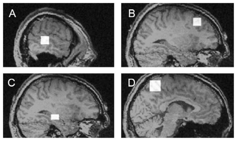
Examples of 4 ROIs to which simulated data was added: (A) left temporal lobe (3 × 3 × 3 voxels), (B) right frontal lobe (3 × 3 × 3 voxels), (C) right hippocampus (2 × 2 × 3 voxels), (D) left parietal lobe (4 × 4 × 4 voxels). Larger versions of each ROI were simulated by increasing each dimension by 1 voxel (i.e. 3 × 3 × 3 would become 4 × 4 × 4 and then 5 × 5 × 5).

Each simulated run contained all 4 forms of epileptic activity (i.e. 1 spike, 5 spikes, 10 spikes, and one 5 s event), one in each ROI. Simulations were repeated 6 times such that the three ROIs containing spikes could simulate each number of spikes twice; simulations of the 5 s event were also repeated 6 times. 756 runs were uniquely simulated (6 control subject scans × 3 ROI sizes × 7 HRF amplitudes × 6 repetitions), for a total of 3024 unique simulated BOLD responses to epileptic activity (4 forms of activity/run × 756 runs). A modified version of the 2D-TCA algorithm (Morgan and Gore, 2009) was then created and its limits were investigated.

Data pre-processing

Pre-processing consisted of slice time correction, motion correction, and spatial smoothing (6 mm FWHM). A brain mask, defined from the anatomical MRI, was created to eliminate voxels outside of the brain; this differs from (Morgan and Gore, 2009) which applied a threshold.

Steps and modifications of the 2D-TCA algorithm

Temporal filtering

While in (Morgan and Gore, 2009) high frequency noise was removed from voxel time courses with a 3-point averaging filter, we applied a rectangular window to a voxel’s frequency spectrum, such that frequencies not expected in a BOLD response were removed. In addition low frequency drift can be removed. As 2D-TCA aims only to detect activity associated with the HRF, the window’s borders are defined according to its spectrum. Fig. 2 shows the spectra of the Glover HRF, and of the Glover HRF convolved with an 8 s step function. The low cut-off frequency of the window can then be defined by the low −3 dB mark on the 8 s event spectrum (0.006 Hz), while the high cut-off frequency can be defined by the high −3 dB mark on the HRF spectrum (0.085 Hz). Although this window is applied, the mean value of the time course (the 0 Hz component) is not removed so that the next step, data normalization, can be effectively carried out.

Figure 2.

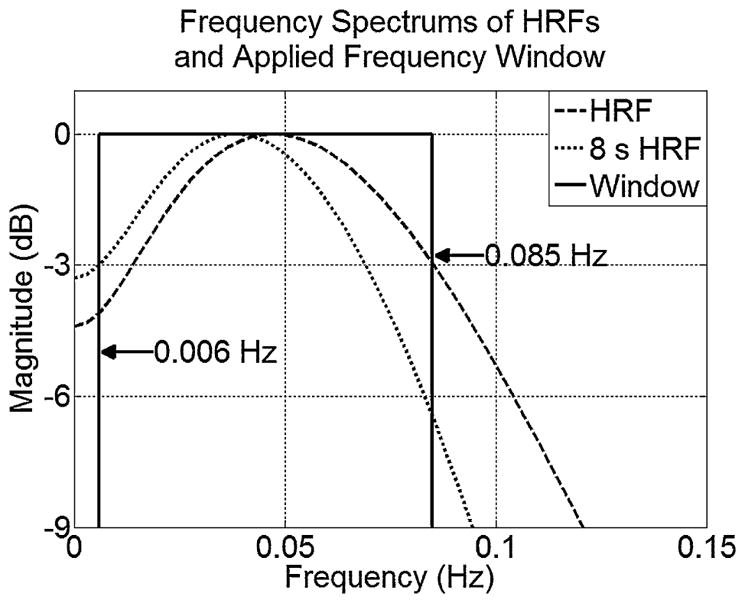
Plots of HRF frequency spectra with indicated rectangular window cut-off frequencies.

Baseline definition and normalization

Morgan and Gore (2009) normalizes a voxel’s time course by the average of its first 5 values. This technique is not very robust as it assumes a patient is at baseline during the first 5 frames, which may not be true. A technique was employed that clustered a voxel’s time course into high and low values via k-means; the mean of the lower cluster was used to estimate baseline. While this technique may impose a slight negative bias on the estimate, it is more effective than using the voxel’s mean value (Fig. 3).

Figure 3.

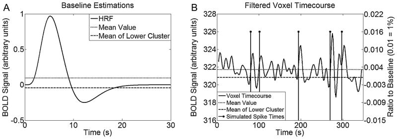
(A) Estimates of baseline for the Glover HRF using the mean and through use of the k-means clustering process. (B) Example of applying k-means to define the baseline value used to normalize a time course containing simulated spikes (right y-axis indicates normalized scale).

Detection of candidate voxels

In Morgan and Gore (2009), voxels that may contain responses to epileptic activity are detected by defining a range (0.5–8% above baseline) within which BOLD signal changes of interest are expected to be. If a voxel’s maximum value is within this range the voxel is considered as a “candidate” while others are considered as “global”.

In this study a number of range boundaries were tested. Lower boundary values (0, 0.5, 1, 1.5, and 2% above baseline) were chosen based on BOLD response amplitudes expected to result from epileptic activity, while upper boundary values (3–11% above baseline in increments of 1%) were chosen to border the 8% value implemented in Morgan and Gore (2009). All range combinations were tested on all simulated runs to determine their ability to label voxels that contained simulated activity as candidates. The best range was determined as that which provided the best average specificity across all runs while maintaining an average sensitivity of 90%. This range was between 1 and 6% above baseline and provided a true positive rate (TPR) of 0.90 and false positive rate (FPR) of 0.59. As implemented in Morgan et al. (2008), a global voxel time course was then calculated as the mean time course of all global voxels and subtracted from all candidate voxel time courses to remove global forms of activity or noise.

Event detection and creation of 2D histogram

In Morgan and Gore (2009) an event is detected in a candidate voxel time course anytime the voxel goes over 1.5 standard deviations above baseline. In this study 11 thresholds were tested (0–2 standard deviations in increments of 0.2). The best threshold was determined as that which provided a maximum average specificity while maintaining an average sensitivity of at least 90%. This value was 1.2 standard deviations and provided a TPR of 0.91 and FPR of 0.29. In addition, although not implemented in Morgan and Gore (2009), a spatial constraint was imposed and consisted of counting an event in a voxel only if events were detected at the same time in 4 of the voxel’s 6 closest neighbours. By incorporating this condition those events that may occur due to spatially uncorrelated activity, such as white noise, were ignored. This criterion was chosen as it did not seem overly conservative or liberal.

Event time courses were then temporally clustered into a 2D histogram. As in Morgan and Gore (2009), the frame number of a voxel’s maximum value defined to which row in the 2D histogram its event time course was added. After the 2D histogram was created by this means, all null rows were discarded.

Grouping similar rows in the 2D histogram

Each row of the 2D histogram describes underlying activity common to many voxels. However, it is probable that multiple rows describe the same activity as voxels associated with similar activity may peak at different times due to slight variations in their time courses. The rows that describe similarly timed activity should be grouped.

Grouping was carried out in two steps. The first compared the time courses of all rows to one another and summed those whose correlation coefficient was above a threshold. A range of thresholds (0–1 in increments of 0.1) was tested on all simulated runs. To determine the performance of each threshold value, t-maps, thresholded at t > 3.1 (P < 0.001), were created from each of the grouped histograms that resulted from applying a given threshold. Those t-maps whose regions of activation best described the four simulated ROIs in a given run, determined by their TPR (associated FPR was negligible), were selected and the overall TPR associated with the given threshold was calculated as the number of true positives in those t-maps divided by the number of voxels known to be active in that run. The best threshold was then that which performed the most grouping while maintaining a reasonable TPR. As the TPR started to severely decline at a threshold of 0.7 (Fig. 4(A)), a threshold of 0.8 was selected. This provided an average TPR of 0.81 and an average FPR, which for a run was calculated as the average of the FPRs of the four selected t-maps, of 0.012. With this threshold an average of 140 rows remained (with no grouping there were 183).

Figure 4.

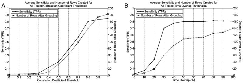
Average TPR and number of rows created for (A) tested correlation coefficient threshold values, and (B) time overlap threshold values.

Grouping by correlation is not sufficient as rows that describe similar activity, but whose peaks occur at distant time points, are not grouped. The second grouping step accounts for this and consisted of applying a threshold to each row, equal to the mean of its non-zero values, and grouping those rows whose activity above threshold overlapped for a certain percentage of their combined time of activity. A range of time overlap percentages (0–100% in increments of 10%) were tested on all simulated runs with performance determined by the same technique as for the first grouping step. As the TPR started to severely decline at a threshold of 20% (Fig. 4(B)), a threshold of 30% was selected. This provided an average TPR across all simulated runs of 0.70 and an average FPR of 0.026. By applying this threshold an average of 59 rows remained.

Removal of insignificant rows

In Morgan and Gore (2009) the mean and standard deviation of maximum values across all rows were calculated. Rows whose maximum value was at least 1 standard deviation above the mean were then considered as significant components and were retained. Applying this threshold, this study found that components describing simulated activity were often inappropriately discarded. A lower threshold, applied to the actual peak number of events in a row, was used such that insignificant rows were removed. A range of thresholds (0–65 events in increments of 5) were tested on all simulated runs with performance being determined by the same technique applied for the grouping steps. As the TPR started to severely decline for a threshold of 20 events or higher, a threshold of 15 events was selected. This provided an average TPR of 0.65 and an average FPR of 0.029. By applying this threshold an average of 15 rows remained.

Creation of t-maps

Rows remaining from the previous step were passed, along with motion correction parameters, to the GLM (Worsley et al., 2002) (the HRF used was a version of the Glover HRF, positioned such that the peak occurred at time 0) to obtain their t-maps. These maps were thresholded at t > 3.1 (corresponding to P < 0.001) to determine regions of activation. Various spatial extent thresholds were then applied to regions of activation to determine if this would help identify those which described epileptic activity.

Selection and analysis of patient data

Patient runs used to test 2D-TCA were selected to match the characteristics of simulated activity (i.e. event frequency, HRF amplitude, and ROI size) for which 2D-TCA was found to provide effective detection. The procedure for selecting patient data will therefore be given after the results of the simulation study.

2D-TCA’s ability to detect epileptic activity in patient runs was determined by qualitatively comparing results to EEG-fMRI results for the same runs. Cases in which 2D-TCA created a t-map that described what was seen by EEG-fMRI were investigated by a neurologist who was asked to consider the results of 2D-TCA as a substitute for EEG-fMRI. This was done by blinding the neurologist to the EEG-fMRI results, but allowing them to have full access to all other patient data (i.e. routine EEG, anatomical MRI, clinical data, etc.). They were then asked to rank each 2D-TCA created component, on a scale of 1–5, based on the probability that it described epileptic activity in the given patient, 1 indicating a component that definitely did not arise from epileptic activity, 3 indicating a component whose source was unclear, and 5 indicating a component that most likely arose from epileptic activity (2 and 4 were intermediary values).

Results

Performance in detecting simulated activity

Ideally, 2D-TCA would only create t-maps that describe ROIs containing simulated activity. However, the final output of 2D-TCA may also include t-maps that describe other transient activity. It is therefore important to determine whether within this larger set of t-maps there is one that corresponds to each of the four ROIs simulated in a run (i.e. four t-maps, each describing a different ROI). Fig. 5(A)–(D) shows the average TPR (calculated across all runs containing the specified simulated activity) for the t-map whose region of activation best described the given form of activity simulated in each run, i.e. that t-map which had the highest TPR for the associated ROI (the corresponding FPR values of voxels within the brain were all very small, on the order of 0.01). As the effect of ROI size is of more interest to us than ROI location, TPRs in detecting the left temporal lobe and right frontal lobe ROIs (denoted by T and F in Fig. 5(A)–(C) respectively) have been grouped into the same rows since they were simulated with the same ROI sizes. While in all cases an increase in the simulated HRF amplitude lead to an increase in TPR, an increase in the ROI size had nearly no effect (in fact, no major trend associated with ROI size had been expected). Fig. 5(E) shows the same data as Fig. 5(A)–(D) except collapsed across ROI sizes. It was decided that for effective and consistent detection of a given form of activity, 2D-TCA should produce an average TPR of at least 0.95. Therefore, for effective detection, 1 spike per run is insufficient, while 5 spikes per run requires an HRF amplitude of at least 1.5% above baseline (TPR of 0.999), 10 spikes per run at least 1.25% (TPR of 0.959), and one 5 s event at least 1% (TPR of 0.976).

Figure 5.

TPR in detecting simulated activity of different HRF amplitudes and ROI sizes in the case of (A) 1 spike per run, (B) 5 spikes per run, (C) 10 spikes per run, and (D) one 5 s event per run. Labels T, F, and H indicate brain areas containing the ROI (T = left temporal lobe, F = right frontal lobe, and H = left hippocampus; 5 s event was only simulated in right parietal lobe; T and F ROIs are grouped in (A)–(C) as they were simulated with the same ROI sizes). (E) Shows the same information on one plot by collapsing each plot in (A)–(D) across ROI size.

Although 2D-TCA created components that precisely described activity simulated with these characteristics, it also created other components that contained significant activation. Fig. 6 is a box plot showing, for runs simulated with an HRF amplitude of 1% or larger (i.e. the minimum HRF amplitude for which simulated activity was consistently detected), the number of t-maps that contained clusters of activation larger than a range of sizes. While increasing the cluster size threshold lead to fewer and fewer considered t-maps, even when a threshold of 220 voxels was applied, which was larger than the largest simulated ROI (216 voxels), up to 3 t-maps still contained significant activation that, in some cases, could be misinterpreted as arising from epileptic activity.

Figure 6.

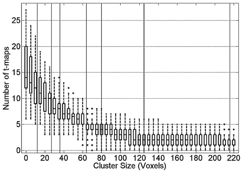
Number of components whose activation maps have cluster sizes above various threshold levels. Vertical black lines indicate the simulated epileptic activity ROI sizes (i.e. 12, 27, 36, 64, 80, 125, and 216).

Selection of patient data

A patient run was analyzed with 2D-TCA if its EEG-fMRI results showed clear activation that had characteristics similar to the consistently detectable forms of simulated activity described above. However, to increase the number of patient runs, these criteria were slightly relaxed. Therefore, a run was selected if it included at least 4 spikes or multiple prolonged events whose total duration was between 3 and 8 s, and if the HRF amplitude associated with the activity, found from the EEG-fMRI results, was at least 0.9% above baseline. Sixty runs, 40 containing spikes and 20 containing prolonged events, were selected from the first 20 patients who met these criteria from a pool of 43 patients.

Performance in detecting epileptic activity in patients

Table 1 shows the performance of 2D-TCA, as compared to EEG-fMRI, in detecting spikes in patient runs (each row represents a run) after cluster size thresholds of 15, 50, 100, and 200 have been applied to resulting t-maps. Table 2 shows the performance in detecting longer events for the same cluster size thresholds in addition to thresholds of 500 and 1000, added based on the cluster sizes of EEG-fMRI results associated with long events; both tables also give the characteristics of the epileptic activity recorded in the run. A case in which 2D-TCA produced a t-map that passed the given cluster size threshold and that closely resembled what was seen in the EEG-fMRI results (Fig. 7) is indicated in light grey, while a case in which no similarity was seen is indicated in dark grey. Medium grey indicates a case in which one of the t-maps largely overlapped with the EEG-fMRI results but did not include the maximum t-valued voxel (Fig. 8). Also given is the number of components initially created by 2D-TCA and the number of t-maps that remained after the cluster size thresholds were applied.

Table 1.

Performance of 2D-TCA in detecting spikes in patient runs when different cluster size thresholds are applied. Runs are sorted by EEG-fMRI activation size from highest to lowest.

Epileptic Activity Characteristics (obtained from EEG-fMRI data)				2D-TCA Results
Patient #	# of spikes	HRF Amplitude (% above baseline)	Size (voxels)	# of components	# of t-maps with activity	# of t-maps with cluster size of:
						15	50	100	200
1	6	1.81	762	14	11	10	8	7	4
1	17	1.03	733	9	8	7	6	4	3
2	13	1.81	710	16	10	10	10	9	6
3	5	1.53	697	3	3	2	1	0	0
4	4	1.18	623	2	1	1	1	0	0
5	4	1.45	507	28	18	15	12	8	5
6	6	1.06	478	1	1	0	0	0	0
7	18	1.87	424	2	2	2	2	2	2
8	5	1.86	219	6	8	6	4	4	3
9	5	1.36	201	9	8	6	4	2	1
2	4	1.13	164	15	8	6	6	5	4
1	7	0.99	155	7	3	3	3	3	1
2	4	1.69	152	10	4	4	4	4	2
2	5	1.56	132	14	6	5	4	3	3
10	4	0.94	127	9	6	4	4	2	1
11	11	1.75	114	3	2	2	1	0	0
12	8	1.83	106	11	8	6	3	3	3
5	7	1.65	102	10	8	8	8	6	5
6	13	1.58	100	3	2	2	2	1	1
4	15	1.31	99	2	1	0	0	0	0
5	15	1.22	98	7	6	6	3	2	2
13	5	1.68	97	7	6	6	4	3	2
1	14	1.64	84	6	3	3	3	3	3
1	18	1.29	82	7	6	5	5	5	1
7	30	1.07	81	6	3	3	3	2	0
13	6	1.61	78	3	3	3	3	2	2
5	4	2.12	69	13	8	7	4	2	1
4	9	2.05	63	4	3	2	0	0	0
3	4	1.18	60	4	2	2	2	2	2
10	5	1.92	51	2	2	2	1	0	0
2	5	1.3	42	6	5	4	3	2	1
14	7	1.73	36	10	5	5	2	1	0
11	9	1.59	33	3	3	1	1	0	0
11	5	1.22	29	9	8	7	2	2	2
4	4	1.72	27	8	2	2	1	1	0
8	5	1.85	26	8	6	5	4	1	0
9	9	1.34	25	3	2	2	2	2
15	10	1.26	23	13	11	8	7	5	2
16	8	0.95	19	15	8	6	6	6	3
8	6	1.64	17	17	10	10	7	5	4

Table 2.

Performance of 2D-TCA in detecting longer interictal events when different cluster size thresholds are applied. Runs are sorted by number of events detected in the EEG from highest to lowest.

Epileptic Activity Characteristics (obtained from EEG-fMRI data)						2D-TCA Results
Patient #	# of events	Average event duration (s)	Total time active (s)	HRF Amplitude (% above baseline)	Size (voxels)	# of components	# of t-maps with activity	# of t-maps with cluster size of:
								15	50	100	200	500	1000
17	18	2.97	53.46	1.42	3341	10	7	6	6	6	4	1	0
17	9	3.19	28.71	1.33	3159	11	10	10	9	6	6	2	0
17	7	3.16	22.12	1.72	2845	13	13	8	6	3	2	2	0
7	4	2.65	10.6	1.14	1385	5	5	5	5	4	3	2	0
18	3	6.6	19.8	1.75	6469	5	3	2	2	2	2	0	0
19	3	2.63	7.89	1.36	3843	11	9	9	7	5	3	0	0
7	3	2.27	6.81	1.23	1312	18	6	5	3	3	2	1	1
17	2	6.3	12.6	3.01	3478	8	8	7	5	4	4	1	0
20	2	2.57	5.14	1.95	726	14	11	10	6	4	3	2	1
20	2	2.38	4.76	1.08	621	13	13	8	3	3	1	0	0
19	2	4.7	9.4	1.58	3678	10	8	7	6	5	4	1	0
19	2	3.8	7.6	1.28	3556	6	3	3	3	2	2	1	0
17	1	3.1	3.1	1.29	2142	6	6	5	3	3	2	0	0
1	1	4.2	4.2	2.41	71	8	8	7	5	4	4	3	1
20	1	4.07	4.07	1.06	597	3	3	3	2	2	2	1	0
7	1	6.2	6.2	1.22	1440	5	5	2	2	1	0	0	0
17	1	5	5	1.12	2798	7	6	5	2	2	1	1	0
19	1	4.5	4.5	1.07	3802	4	2	2	1	1	1	0	0
7	1	3.4	3.4	1.45	1189	16	13	10	4	3	3	0	0
7	1	3.5	3.5	1.29	845	16	10	10	5	2	2	0	0

Figure 7.

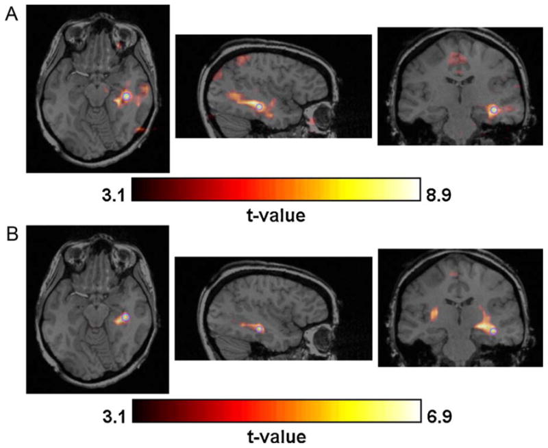
Example of strong concordance (indicated by light grey in Tables 1 and 2) between the t-map created by (A) EEG-fMRI and (B) one of the 2D-TCA components. The purple circle indicates the exact voxel whose slices are shown. (For interpretation of the references to color in this figure legend, the reader is referred to the web version of the article.)

Figure 8.

Example of some overlap (indicated by medium grey in Tables 1 and 2) between the t-map created by (A) EEG-fMRI and (B) one of the 2D-TCA components. The purple circle indicates the exact voxel whose slices are shown. Note frontal lobe activity in the sagittal slice of the EEG-fMRI map and its absence in the 2D-TCA map. (For interpretation of the references to color in this figure legend, the reader is referred to the web version of the article.)

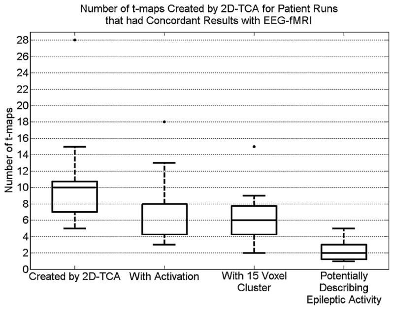
Table 1 shows that in most cases 2D-TCA did not effectively detect spike activity found by EEG-fMRI, although there may have been a slight dependence on activation size. Table 2 on the other hand shows that 2D-TCA was able to effectively detect what was found by EEG-fMRI when a run contained at least two long interictal events, each on the order of a few seconds, while if only one event occurred it was essentially undetectable. For runs in which 2D-TCA created a t-map that described what was seen by EEG-fMRI (i.e. light and medium grey cells), applying increasing cluster size thresholds generally did not result in a deterioration of performance but did reduce the number of considered t-maps. Fig. 9(A) shows a box plot of the number of t-maps created for the 40 patient runs that contained spikes, as well as the number that showed activity in the brain and the number that contained clusters larger than the applied thresholds; Fig. 9(B) shows the same data for the 20 runs that contained longer events. In an ideal case, by applying these thresholds only a single t-map would remain and that t-map would describe the epileptic activity. For 8 of the 15 runs in which similar activity was detected (light grey cells in Tables 1 and 2), that map which closely described the EEG-fMRI results contained the largest cluster of activity of all 2D-TCA maps created for that run; however, in the 7 other cases at least one other t-map contained an activation cluster consisting of more voxels than the detected epileptic activity. Looking at Fig. 9(A) it can be seen that, for runs that contained spikes, even when a cluster size threshold of 200 voxels is applied up to 6 t-maps remained in one case. Likewise, for runs that contained prolonged events, when a cluster size threshold of 500 voxels is applied up to 3 t-maps can remain.

Figure 9.

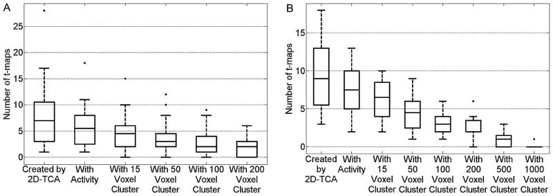
Box plot showing, for (A) the 40 patient runs containing spikes and (B) the 20 patient runs containing prolonged events, the number of t-maps created, number of those created that contain activity in the brain, and number of those that contain a cluster of activity larger than the applied threshold levels.

Among 2D-TCA created t-maps that did not describe epileptic activity, two were found to be common for a number of runs from different patients. The first, which occurred in 14 of the 60 runs, consisted of activation within or close to the ventricles. The second, which occurred in 12 of the runs, consisted of bilateral activity close, often slightly posterior, to the central sulcus (Fig. 10).

Figure 10.

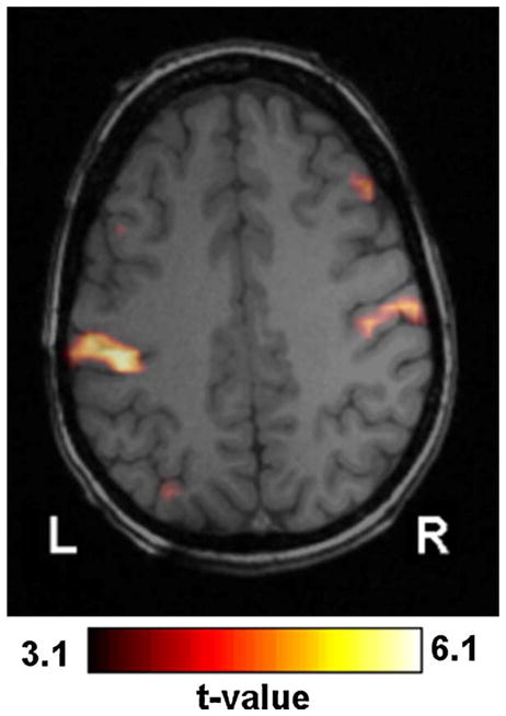
Example of commonly found activation near (in this case slightly posterior to) the central sulcus.

Analysis by neurologist

The t-maps from runs for which 2D-TCA created one t-map that closely described what was seen in the EEG-fMRI results (i.e. 16 light grey rows in Tables 1 and 2; only t-maps created for these runs that had a activation size of at least 15 voxels were considered) were given to a neurologist for further analysis. This was done to determine, without the knowledge of EEG-fMRI results, the number of t-maps created by 2D-TCA that may be interpreted as describing the epileptic activity of a given patient and the number that can be ignored because they show regions of activation that are highly unlikely to be generated by the patient’s epileptic activity. While for all runs it was known that only one of the 2D-TCA created t-maps closely described the EEG-fMRI results, the neurologist found that a median of 2 and a maximum of 5, each describing a different region of activation, could not be ignored and could be considered as potentially arising from epileptic activity (Fig. 11). For five of these runs the neurologist gave a score of 4 or 5 to a t-map that showed similar activation as the EEG-fMRI results, while in three other runs they gave a score of 4 to a t-map that was known not to show similar activity to what was obtained by EEG-fMRI; the neurologist gave a maximum score of 3 for t-maps created for the remaining 8 runs.

Figure 11.

Box plot showing, for runs for which 2D-TCA created a t-map that closely described what was seen in the EEG-fMRI results, the number of t-maps created, number of those created that contain significant activity in the brain, number of those with a cluster of activity of 15 voxels or larger, and number that, in the opinion of the neurologist, could not be ignored and therefore could describe epileptic activity.

Discussion

The main advantage to localizing epileptic activity in fMRI data, for example by EEG-fMRI, is the ability to do so throughout the entire brain with high spatial precision. If this can be done without dependence on events detected in a simultaneously recorded EEG, the scanning process would be more manageable and activity restricted to deep brain structures, undetectable by EEG, may be detected. This study investigated the ability of 2D-TCA, a method that detects transients in fMRI data independently of EEG, to detect BOLD signal changes resulting from epileptic activity of various forms in simulated and patient data. Characteristics investigated included event frequency/duration, spatial extent, and HRF amplitude. When applied to simulated data, 2D-TCA functioned similarly in detecting activity of various spatial extents, but could only consistently detect activity containing 5 spikes/run with an associated HRF amplitude of at least 1.5% above baseline, 10 spikes/run with an HRF amplitude of at least 1.25%, or one 5 s long event with an HRF amplitude of at least 1%. When applied to patient data that contained activity apparently similar to the detectable simulated activity, only activity for which the EEG showed multiple prolonged events (each on the order of a few seconds) could be consistently detected by 2D-TCA, while the detection of interictal spikes, although in some cases very accurate, was inconsistent. This superior performance in detecting longer events may not only be due to the longer duration of activation, but also because for the same HRF, a prolonged event will cause a larger change in the BOLD signal than a spike. It is also interesting to note that t-maps created by 2D-TCA, which showed very similar activation to what was obtained by EEG-fMRI, often had more focal activation regions than their EEG-fMRI counterparts. This may indicate that 2D-TCA is more sensitive to the initial source of epileptic activity than EEG-fMRI is, a quality that would require further investigation.

The issue then arises: if 2D-TCA only detects epileptic activity that has the above described characteristics which, in the case of a patient, are uncontrollable, how can it be determined, in the absence of EEG, if activity is expected to be detected in a given patient? In fact, given these conditions, this would not be possible. Rather, the above described characteristics, which concern the HRF amplitude and frequency/length of the activity, might be incorporated into the analysis of the 2D-TCA generated t-maps. For example, the HRF amplitude associated with activity described in each t-map could be calculated by taking the average peak amplitude of all voxels that are clustered to the same final component. Those components for which the HRF amplitude is not deemed as sufficient could then be ignored. To determine whether or not activity described by a given t-map consisted of frequent and/or long enough activity one would simply have to look at the time course of the component used to create that t-map. If the time course did not describe frequent or long enough activity, its corresponding t-map could be ignored.

Another possible method to reduce the number of considered t-maps would be to apply a cluster size threshold. For cases in which 2D-TCA created a t-map that closely described what was seen by EEG-fMRI, applying larger and larger cluster size thresholds led to fewer and fewer t-maps, but retained that which described the epileptic activity. Unfortunately, as the size of a patient’s region of activation is not known before hand, it is hard to determine an optimal cluster size threshold. It would also be inappropriate to simply select the t-map that showed the largest activation region as it would not necessarily describe the epileptic activity. The best way may be to reduce the number of considered t-maps by applying a cluster size threshold of 15 (for runs for which results similar to EEG-fMRI were obtained, applying this threshold resulted in a median of 6 t-maps). This reduced set could then be investigated by a neurologist to determine t-maps with activity of interest. This study found that while a neurologist is able to ignore some of the maps because they describe activation regions unlikely to be associated with a patient’s epilepsy, in most cases more than one will remain, leading to uncertainty. In addition, for 5 of the 16 runs for which 2D-TCA created a t-map that closely described the EEG-fMRI results, the blinded neurologist could not confidently qualify that t-map as describing the patient’s epilepsy. This lack of confidence in determining which t-maps are associated with epilepsy results from 2D-TCA’s lack of specificity to epileptic activity (EEG-fMRI achieves this specificity by finding BOLD correlates to epileptic activity in the EEG). 2D-TCA can only be effectively used to validate localization by other means or to create hypotheses as to where epileptic activity may be occurring.

Causes of commonly generated maps

It is believed that ventricle activation, which was commonly generated for a number of runs from different patients, may describe BOLD signal changes arising from residual movement artifacts, the patient’s respiration, or the patient’s heartbeat as the ventricles are susceptible to these forms of noise (Windischberger et al., 2002). Activation around the central sulcus, which was also generated for different patients, may describe motor or somatosensory activity that occurred in the patient, or was imagined by them. This region is very similar to the motor cortex activation commonly observed in (Morgan et al., 2008). The systematic elimination of such maps would reduce the number of maps to consider in the final analysis.

Advantages compared to EEG-fMRI

One of the advantages of 2D-TCA compared to EEG-fMRI is its potential to detect activity restricted to deep brain structures. While this was evident when 2D-TCA was applied to the simulated data (i.e. detection of activity in the hippocampal ROI), it was not as clear from the patient data. For example, in three patient runs 2D-TCA created a t-map that was not similar to the EEG-fMRI results, but, according to the blind neurologist, could describe epileptic activity; however, it is expected that activation areas in all three cases should have been detected in the EEG as all were relatively superficial and consisted of an activated area of cortex larger than the minimum 10 cm² required for EEG detection (Tao et al., 2007) (why similar regions were not detected by EEG-fMRI may be a result of inadequate EEG markings, or indicative that these regions were in fact not associated with epileptic activity). As such, 2D-TCA’s potential to detect activity restricted to deep brain structures in patient data was not confirmed.

Another point to consider is the fact that EEG-fMRI requires one to impose the delay of the HRF, which can differ between people or brain structures (Aguirre et al., 1998). Some techniques try to overcome this problem by processing the same fMRI data with multiple HRFs of different delay. 2D-TCA requires no such assumption as it detects events from the BOLD signal itself; only the exact shape of the HRF must be assumed, something that does not show as much variability.

Comparison to independent component analysis

Although independent component analysis (ICA) was not carried out in this study, the performance of 2D-TCA in detecting transient BOLD activity as compared to ICA has been previously investigated by Morgan et al. (2008). They found that detection by 2D-TCA was comparable to that by ICA (2D-TCA provided slightly worse sensitivity), but with significantly fewer detected components (on the order of 5 compared to 10 or 100) and hence a higher specificity. Based on the 2D-TCA results we obtained in this study and the findings of Morgan et al., we would predict a similar outcome; that is, applying ICA to the data used in this study would in fact provide better sensitivity than 2D-TCA did, but the number of extra components it creates compared to the number created by 2D-TCA makes 2D-TCA the more practical technique of the two.

Conclusion

This study investigated the ability of 2D-TCA to effectively detect epileptic activity of various forms in both simulated and patient fMRI data. It was found that if enough events were recorded during an fMRI run and the HRF associated with those events was of adequate amplitude, 2D-TCA could consistently detect epileptic activity. However, due to its lack of specificity to epileptic activity, 2D-TCA also created maps describing other activity not associated with epilepsy, some of which could not be ignored, leading to uncertainty in the results. It was therefore concluded that 2D-TCA can only be used to validate localization of epileptic activity by other means or to create hypotheses as to where this activity may be occurring.

References

- Aguirre GK, Zarahn E, D’Esposito M. The variability of human, BOLD hemodynamic responses. Neuroimage. 1998;8:360–369. doi: 10.1006/nimg.1998.0369. [DOI] [PubMed] [Google Scholar]
- Allen PJ, Josephs O, Turner R. A method for removing imaging artifact from continuous EEG recorded during functional MRI. Neuroimage. 2000;12:230–239. doi: 10.1006/nimg.2000.0599. [DOI] [PubMed] [Google Scholar]
- Benar C, Aghakhani Y, Wang Y, Izenberg A, Al-Asmi A, Dubeau F, Gotman J. Quality of EEG in simultaneous EEG-fMRI for epilepsy. Clin Neurophysiol. 2003;114:569–580. doi: 10.1016/s1388-2457(02)00383-8. [DOI] [PubMed] [Google Scholar]
- Engel J., Jr A practical guide for routine EEG studies in epilepsy. J Clin Neurophysiol. 1984;1:109–142. doi: 10.1097/00004691-198404000-00001. [DOI] [PubMed] [Google Scholar]
- Glover GH. Deconvolution of impulse response in event-related BOLD fMRI. Neuroimage. 1999;9:416–429. doi: 10.1006/nimg.1998.0419. [DOI] [PubMed] [Google Scholar]
- Gotman J, Kobayashi E, Bagshaw AP, Benar CG, Dubeau F. Combining EEG and fMRI: a multimodal tool for epilepsy research. J Magn Reson Imaging. 2006;23:906–920. doi: 10.1002/jmri.20577. [DOI] [PubMed] [Google Scholar]
- Hamandi K, Salek Haddadi A, Liston A, Laufs H, Fish DR, Lemieux L. fMRI temporal clustering analysis in patients with frequent interictal epileptiform discharges: comparison with EEG-driven analysis. Neuroimage. 2005;26:309–316. doi: 10.1016/j.neuroimage.2005.01.052. [DOI] [PubMed] [Google Scholar]
- Liu Y, Gao JH, Liotti M, Pu Y, Fox PT. Temporal dissociation of parallel processing in the human subcortical outputs. Nature. 1999;400:364–367. doi: 10.1038/22547. [DOI] [PubMed] [Google Scholar]
- Liu Y, Gao JH, Liu HL, Fox PT. The temporal response of the brain after eating revealed by functional MRI. Nature. 2000;405:1058–1062. doi: 10.1038/35016590. [DOI] [PubMed] [Google Scholar]
- Morgan VL, Gore JC. Detection of irregular, transient fMRI activity in normal controls using 2dTCA: comparison to event-related analysis using known timing. Hum Brain Mapp. 2009;30:3393–3405. doi: 10.1002/hbm.20760. [DOI] [PMC free article] [PubMed] [Google Scholar]
- Morgan VL, Gore JC, Abou-Khalil B. Cluster analysis detection of functional MRI activity in temporal lobe epilepsy. Epilepsy Res. 2007;76:22–33. doi: 10.1016/j.eplepsyres.2007.06.008. [DOI] [PMC free article] [PubMed] [Google Scholar]
- Morgan VL, Gore JC, Abou-Khalil B. Functional epileptic network in left mesial temporal lobe epilepsy detected using resting fMRI. Epilepsy Res. 2010;88:168–178. doi: 10.1016/j.eplepsyres.2009.10.018. [DOI] [PMC free article] [PubMed] [Google Scholar]
- Morgan VL, Li Y, Abou-Khalil B, Gore JC. Development of 2dTCA for the detection of irregular, transient BOLD activity. Hum Brain Mapp. 2008;29:57–69. doi: 10.1002/hbm.20362. [DOI] [PMC free article] [PubMed] [Google Scholar]
- Morgan VL, Price RR, Arain A, Modur P, Abou-Khalil B. Resting functional MRI with temporal clustering analysis for localization of epileptic activity without EEG. Neuroimage. 2004;21:473–481. doi: 10.1016/j.neuroimage.2003.08.031. [DOI] [PubMed] [Google Scholar]
- Tao JX, Baldwin M, Hawes-Ebersole S, Ebersole JS. Cortical substrates of scalp EEG epileptiform discharges. J Clin Neurophysiol. 2007;24:96–100. doi: 10.1097/WNP.0b013e31803ecdaf. [DOI] [PubMed] [Google Scholar]
- Windischberger C, Langenberger H, Sycha T, Tschernko EM, Fuchsjager-Mayerl G, Schmetterer L, Moser E. On the origin of respiratory artifacts in BOLD-EPI of the human brain. Magn Reson Imaging. 2002;20:575–582. doi: 10.1016/s0730-725x(02)00563-5. [DOI] [PubMed] [Google Scholar]
- Worsley KJ, Liao CH, Aston J, Petre V, Duncan GH, Morales F, Evans AC. A general statistical analysis for fMRI data. Neuroimage. 2002;15:1–15. doi: 10.1006/nimg.2001.0933. [DOI] [PubMed] [Google Scholar]