A Minimal Path Searching Approach for Active Shape Model (ASM)-based Segmentation of the Lung

Abstract

We are developing a minimal path searching method for active shape model (ASM)-based segmentation for detection of lung boundaries on digital radiographs. With the conventional ASM method, the position and shape parameters of the model points are iteratively refined and the target points are updated by the least Mahalanobis distance criterion. We propose an improved searching strategy that extends the searching points in a fan-shape region instead of along the normal direction. A minimal path (MP) deformable model is applied to drive the searching procedure. A statistical shape prior model is incorporated into the segmentation. In order to keep the smoothness of the shape, a smooth constraint is employed to the deformable model. To quantitatively assess the ASM-MP segmentation, we compare the automatic segmentation with manual segmentation for 72 lung digitized radiographs. The distance error between the ASM-MP and manual segmentation is 1.75 ± 0.33 pixels, while the error is 1.99 ± 0.45 pixels for the ASM. Our results demonstrate that our ASM-MP method can accurately segment the lung on digital radiographs.

INTRODUCTION

X-ray imaging is an important means to explore the pathological changes of the chest, including the lung, trachea, bronchia, pleura, vessel, mediastinum, diaphragm, esophagus, soft tissue, and etc. The quality of radiographs varies considerably due to doses, orientation, distance, alignment, and pathology. The images are characterized with contrast variation and non-uniform intensity background [1], which introduces difficulty for accurate segmentation and quantitative analysis in routine clinical practice.

The deformable contour model such as active contours or snakes (Kass et al.,1988) [1] and other deformable models are capable of capturing the complexity and the variability of the shape of anatomical objects in medical images. These models can be sensitive to initial positions, especially for noise images. It can be difficult to deal with topological adaption because of no constraint on the overall shape [2][3][4].

Active shape models (ASM) combine the deformable shape descriptors with statistical model analysis. Object shapes are represented by a mean shape from the boundary points using principal component analysis (PCA). Thus, the deformations are modeled using a linear combination of the eigenvectors of the variations from the mean shape. It iteratively refines the pose and shape parameters of the point distribution model and updates the target points using a fitting criterion, i.e. the least Mahalanobis distance. However, the displacement is determined by a search only along the normal direction toward the strongest image edge. Moreover, the target points are determined by each contour point independently and it leads to a wrong boundary if an appropriate target point is selected during the searching procedure [5]–[6].

In order to overcome these limitations, we extend the searching direction to a fan-shape region and construct a cost function, which is minimized by a minimal path method using dynamic programming. A statistical prior shape is incorporated into the minimal path deformable model. Bayesian maximal a posteriori (MAP) is introduced into the contour detection processing. Smoothness constraints are imposed to keep the continuousness of the shape. A smooth item is incorporated into the covariance matrix of training points with regard to the correlation of neighboring points.

SEGMENTATION METHODS

Active shape models

An object is described by n points, referred as landmark points. The landmark points are determined manually in a set of s training images. For example, we can represent n landmark points, {(x_i, y_i)} as the 2n element vector x, where

$$\mathbf{X}={(x_1,y_1,\dots ,x_n,y_n)}^T$$ (1)

Principal component analysis (PCA) is applied to the shape vector x by computing the mean shape

$$\overline{\mathbf{X}}=\frac{1}{s}\sum _{i=1}^n{\mathbf{x}}_i$$ (2)

The covariance is described as:

$$\mathbf{S}=\frac{1}{s-1}\sum _{i=1}^n({\mathbf{x}}_i-\overline{\mathbf{x}}){({\mathbf{x}}_i-\overline{\mathbf{x}})}^T$$ (3)

The eigenvectors Φ_i of S is corresponding to the eigenvalue λ_i (sorted so that λ_i ≥ λ_i+1). For any training set x, we can approximate x using

$$\mathbf{x}\approx \overline{\mathbf{x}}+\mathbf{\Phi }\mathbf{b}$$ (4)

where Φ= (φ₁|φ₂|…|φ_t) and b is a vector of t elements containing the model parameters giving by

$$\mathbf{b}={\mathbf{\Phi }}^T(\mathbf{x}-\overline{\mathbf{x}})$$ (5)

When fitting the model to a set of points, the values of b are constrained to lie within the range $\pm k\sqrt{{\lambda }_i}$, where k usually has a value between 2 and 3.

The number t of eigenvalues is chosen so as to have a certain proportion f_v of the variance in the training shapes, which is usually between 90% and 98%. The desired number of nodes is given by the lest number of eigenvalues so the following criteria is met:

$$\sum _{i=1}^t{\lambda }_i\ge f_v\sum _{i=1}^{2n}{\lambda }_i$$ (6)

Before computing the mean shape, the training shapes are aligned by translating, rotating and scaling. We minimize the weighted sum of squared distances between corresponding points on different shapes. An iterative scheme known as Procrustes analysis is used to align the shapes. Therefore, this alignment procedure makes the shape model independent of the size, position, and orientation of the objects.

However, model points are not always placed at the strongest edge in the locality – they may represent a weaker, secondary edge or other image structures. The key step is how to build statistical models of the image structure and then find the points which best match the model.

A statistical model of the grey-level structure is built along the normal direction of the boundaries in the training set. The intensity derivative along the normal direction is calculated in order to get a set of normalized samples {g _i}. The quality of fitting a new sample g_s to the model is given by

$$f({\mathbf{g}}_s)={({\mathbf{g}}_s-\overline{\mathbf{g}})}^T{S}_g^{-1}({\mathbf{g}}_s-\overline{\mathbf{g}})$$ (7)

Where ḡ and S_g are the mean and covariance of g_i. Equation 7 is the Mahalanobis distance of the sample from the model mean. It is linearly related to the log of the probability of which g_s is drawn from a mean shape distribution. Minimizing f (g_s) is equivalent to maximizing the probability that g_i originates from a multidimensional Gaussian distribution.

However, the displacement of ASM is only determined by a search only along the normal direction toward the strongest image edge. Moreover, the target points are determined by each contour point independently and it leads to a wrong boundary if an appropriate target point is selected during the searching procedure. From our experiments on digital radiographs, we found that sometimes the searching outliers drive the contour far away from the true boundary position, especially for images with special lesions, irregular changes of lung shape. We try to construct a cost function involve all of the target points and minimize the cost path using dynamic programming so as to find the boundary in global instead of finding each point in local of ASM.

Minimal path deformable model

The traditional energy function of snake is proposed by Kass et al [1], includes two important forces. The internal energy controls the smoothness of the contour. The potential energy attracts the contour toward the object boundary. The energy function is described below:

$$E(c)=\alpha {\int }_{\mathbf{\Omega }}{\left|{\mathbf{C}}^{\prime }(\nu )\right|}^{2}d\nu +\beta {\int }_{\mathbf{\Omega }}{\left|{\mathbf{C}}^{″}(\nu )\right|}^{2}d\nu -\lambda {\int }_{\mathbf{\Omega }}\left|\nabla \mathbf{I}(\mathbf{C}(\nu ))\right|d\nu$$ (8)

where α, β and λ denote real positive weighting constants, Ω denotes the current curve, v ∈[0,1] is the parameterization interval for the contour, ∇_I represents the gradient of the image, C is the segmented contour. The energy function can be solved by

$$min{f}_{\mathbf{\Omega }}g{(\left|\nabla \mathbf{I}(\mathbf{C}(\nu ))\right|)}^2•\left|{\mathbf{C}}^{\prime }(\nu )\right|d\nu$$ (9)

where the Euclidean length of the contour C is given by L(C) = f_Ω|C′ (v)| dv= f_Ωds, s∈ [0,1] is also the curve parameter. Therefore, the problem of image segmentation is transformed into a search for the global minimal path.

Maximal a posteriori(MAP) shape model

In order to incorporate the mean shape to the contour searching, a corrected contour can be describe by the maximum a posteriori estimation

$${\mathrm{\Psi }}_{\mathit{MAP}}=\underset{\mathrm{\Psi }}{argmax}p(\mathrm{\Psi }|\mathbf{C},\mathbf{G}(\mathbf{I}))$$ (10)

Where ψ denotes the weighted graph that contains the estimated curve of the object, G(I) is the weighted graph of the image I, we can compute it using Bayes’ Rule[6][11][12]

$$p(\mathrm{\Psi }|\mathbf{C},\mathbf{G}(\mathbf{I}))=\frac{p(\mathbf{C}|\mathrm{\Psi })p(\mathbf{G}(\mathbf{I})|\mathbf{C},\mathrm{\Psi })p(\mathrm{\Psi })}{p(\mathbf{C},\mathbf{G}(\mathbf{I}))}$$ (11)

Where p(C | Ψ) denotes the probability of existence of the curve C, given the estimated shapeΨ. p(G (I ) | C, Ψ) represents the weighted graph G(I), given the curve C and an shape estimation Ψ. The estimated shape, p(Ψ) can be calculated by Gaussian model

$$p(\mathrm{\Psi })=p(\mathbf{b})=\frac{1}{\sqrt{{(2\pi )}^k\left|{\mathrm{\sum }}_k\right|}}exp(\frac{1}{2}{\mathbf{b}}^T{\mathbf{\sum }}_k^{-1}\mathbf{b})$$ (12)

Where Σ is shape variance being composed of corresponding singular values of SVD.

The MAP shape estimation can be calculated by

$${\mathrm{\Psi }}_{\mathit{MAP}}=arg{min}_{\mathrm{\Psi }}\{{\lambda }_1\underset{c}{\int }|\mathrm{\Psi }(\mathbf{C}(s))|ds+{\lambda }_2{\int }_{\mathrm{\Psi }=0}\mathbf{G}(x,y)\mathit{dxdy}+\frac{1}{2}{\mathbf{b}}^T{\mathbf{\sum }}_k^{-1}\mathbf{b}\}$$ (13)

The first term represents the degree of current curve matching the estimated distance map, the second term represents the degree of the estimated distance map matching the former distance map, and the last term represents the probability of the estimated shape ψ.

The MAP shape model is incorporate into the minimal path searching process, we have

$$E(\mathbf{C})=\underset{\mathrm{\Omega }}{\int }(\alpha E_{\mathit{model}}+\beta E_{\mathit{image}}+\gamma E_{\mathit{int}})d\nu$$ (14)

Where E_model, E_image, and E_int denote the prior shape attraction force, the image feature attraction, and the internal force respectively. α, β and γ are real positive weighting constants which balance the forces. E_image is given by

$${\text{E}}_{\text{image}}={\int }_{\mathbf{C}}\left|{\mathbf{C}}_{\text{s}}\right|ds-(1-\lambda ){\int }_{\mathbf{C}}g({\left|\nabla \text{I}(\mathbf{C}(\nu ))\right|}^{2}d\nu$$ (15)

Where the first term denotes the degree of the curve C in the distance map, which is the Euclidean length of the curve C; the second item denotes the gradient of the original image, which is used to regulate the searching when the distance map is not enough for guiding the curve in case of noises and lack of a real edge. λ and (1−λ) denote the weights of the distance and gradient information respectively.

Where E_int can be denoted by

$$E_{\mathit{int}}=\Vert \frac{{\partial }^2\mathbf{C}}{\partial s^2}\Vert$$ (16)

The discrete version is a smooth constraint term denoted by

$$E_{int}=\Vert {\mathbf{P}}_{i-1}-2{\mathbf{P}}_i+{\mathbf{P}}_{i+1}\Vert$$ (17)

Where P is the position of mark point.

Search neighboring region

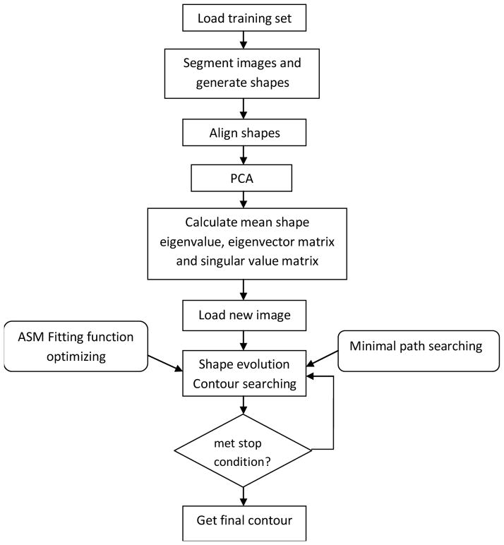
Since there are overlaps and high contrast noises in digital radiographs, model points are not always placed on the strongest edge in the locality – they may represent a weaker secondary edge or some other image structures [5]. Thus the displacements determined by points along the normal direction may lead to a misadjusted boundary if an appropriate target point is selected in the searching processing. We extend the searching in a fan-shape region instead of along the normal direction toward the strongest image edge. The new minimal path cost function is used to find the optimal displacements for landmarks. Figure 1 shows the block diagram of the proposed segmentation algorithm.

Figure 1.

Block diagram of the proposed segmentation algorithm.

Smooth covariance matrix for the mean shape

While the mean shape is calculated from the training set, a smooth constraint is incorporated into the covariance matrix since the identity covariance matrix is too under-constrained if neighboring points are correlated. Like the smooth item in [7], a smooth matrix is applied to generate smoother shapes than those using an identity covariance matrix. The vector of the smooth matrix C_smoth, for k=1, 2, 2n, are given by

$$\begin{array}{l}{\mathbf{q}}_1={(1,0,0.5,0,\dots ,0,0.5,0)}^T\\ {\mathbf{q}}_2={(0,1,0,0.5,\dots ,0,0,0.5)}^T\\ ⋮⋮⋮\\ {\mathbf{q}}_{2n}={(0,0.5,0,0,\dots ,0,0,1)}^T\end{array}$$

The factor 0.5 is adopted to keep the neighboring points to move together and generate smoother shapes than those using the identity covariance matrix.

EXPERIMENTAL RESULTS

Segmentation experiments are carried on 72 patient chest X-ray images to demonstrate the performance of the proposed method. These images were identified by clinical experts and classified into 10 categories, including normal, pneumonia, phthisis, bronchitis, bronchiectasis, pneumothorax, lung cancer, pleural effusion, etc.

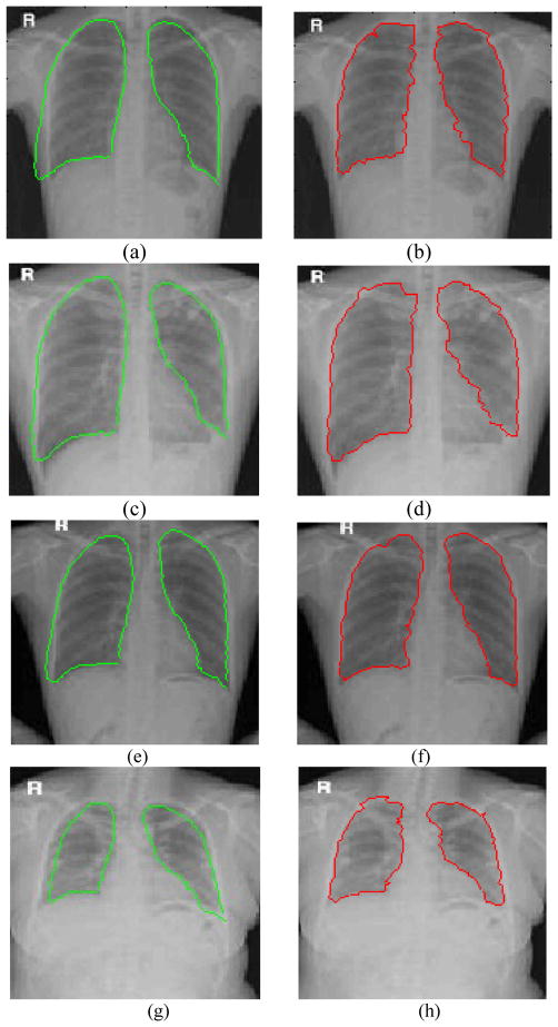
Figure 2 shows the results by the conventional ASM and our ASM-MP. The ASM gives unsatisfactory results due to segmentation errors. The ASM approach usually fails to correct the outliers initialized by the image model, especially the contours of left lung in Fig.2(a), (c), (e) and (g). Fig.2(b), (d), (f) and (h) show that ASM-MP catch the correct outliers after convergence. Although the ASM method has smoother boundaries than the ASM-MP, the ASM-MP can extract the lung more accurately. This can be attributed to the fact that the outliers of smooth initialized shapes are inevitably propagated to the pose and shape by ASM during iteration, the ASM-MP can adjust the outliers and fit the real contours with local features such as gradient and deviation in MP model.

Figure 2.

Segmentation results on chest DR images.

The first and second columns show the results by ASM and ASM-MP, respectively.

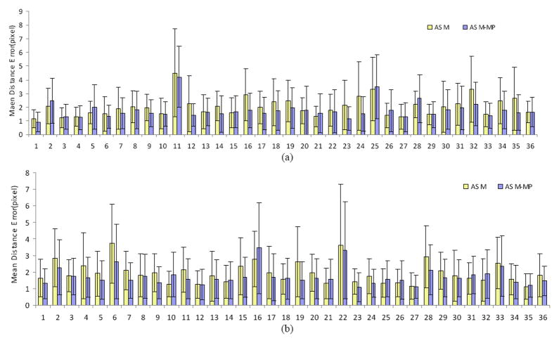
To evaluate our approach, the mean distance error is calculated as a metric to measure the difference between automatic and manual segmentation results as the ground truth. Figure 3 shows the mean distance errors and standard deviation by the ASM and ASM-MP methods. Most of mean distance errors and standard deviation by the ASM-MP are less than that of the ASM, there are still several results with worse measurement such as No 2, 5, 25, 28 in group A and No.10, 16, 21, 31 and 32 in group B. In order to verify if the proposed method has significant improvement for lung segmentation, we performed a paired t-Test for the quantitative measurement. The mean of mean distance errors and standard deviation are 1.75 ± 0.33 and 1.99 ± 0.45 pixels for ASM and ASM-MP, respectively. The p of less 0.001 in a paired t-Test demonstrates that the results from the ASM-MP are significantly different from those of the ASM method.

Figure 3.

Comparison of the mean distance errors and the standard deviation by ASM and ASM-MP for 72 images (e.g., group A, 36 images in (a) and group B, 36 images in (b)). The ASM-MP method has small distance errors for most images compared to the ASM method. A p value of less than 0.001 demonstrates that the two groups are significantly different.

CONCLUSIONS

We developed an automatic searching method for ASM-based segmentation for chest digital radiographic images. In order to minimize the sensitivity of the original ASM approach, we incorporate a smooth constraint to the mean shape and a penalizing outlier strategy, which minimize the cost path using a deformable model. A MAP prior shape estimator is also applied to the deformable model so as to incorporate of the prior shape model to the contours searching procedure. The automatic method can accurately segment the lung on digital radiographs and it outperforms the conventional ASM approach.

References

- 1.Kass M, Witkins A, Terzopoulos Snakes: active contour models. Int Journal Computer Vision. 1988;1(4):321–331. [Google Scholar]
- 2.Greenspan H, Pinhas AT. Medical image categorization and retrieval for PACS using the GMM-KL framework. IEEE Trans on Information Technology in Biomedicine. 2007;11(2):190–202. doi: 10.1109/titb.2006.874191. [DOI] [PubMed] [Google Scholar]
- 3.Durikovic R, Kaneda K, Yamashita H. Dynamic contour: a texture approach and contour operations. The Visual Computer. 1995;11:277–289. [Google Scholar]
- 4.Mcinerey T, Terzopoulos D. Topologically adaptable snakes. Proc. 5th Int’l Conf. Comp. Vis; 1995. pp. 840–845. [Google Scholar]
- 5.Behiels G, Maes F, Vandermeulen D, Suetens P. Evaluation of image features and search strategies for segmentation of bone structures in radiographs using Active Shape Models. Medical Image Analysis. 2002;6:47–62. doi: 10.1016/s1361-8415(01)00051-2. [DOI] [PubMed] [Google Scholar]
- 6.Cootes TF, Taylor CJ, Cooper DH, Graham J. Active shape models- their training and application. Computer Vision and Image Understanding. 1995;61(1):38–59. [Google Scholar]
- 7.Yan PK, Kassim A. Medical Image Segmentation Using Minimal Path Deformable Models With Implicit Shape Priors. IEEE Trans Info Tech in Bio. 2006;10(4):677–684. doi: 10.1109/titb.2006.874199. [DOI] [PubMed] [Google Scholar]
- 8.Wang YM, Staib LH. Boundary finding with correspondence using statistical shape models. IEEE Conf Computer Vision and Pattern Recognition. 1998:338–345. [Google Scholar]
- 9.Benmansour F, Bonneau S, Cohen LD. Finding a Closed Boundary by Growing Minimal Paths from a Single Point on 2D or 3D Images. IEEE Conf Computer Vision. 2007:1–8. [Google Scholar]
- 10.Shi YH, Qi FH, Xue Z. Segmenting Lung Fields in Serial Chest Radiographs Using Both Population-Based and Patient-Specific Shape Statistics. IEEE Trans On Medical Imaging. 2008;27(4):481–494. doi: 10.1109/TMI.2007.908130. [DOI] [PubMed] [Google Scholar]
- 11.Dindoyal I, Lambrou T, Deng J. Automatic segmentation of low resolution fetal cardiac data using snakes with shape priors. Proc. 5th Int’l Conf. Image and signal processing and Analysis; 2007. pp. 538–543. [Google Scholar]
- 12.Li K, Fei B. A New 3D Model-Based Minimal Path Segmentation Method for Kidney MR Images. The 2nd International Conference on Bioinformatics and Biomedical Engineering, ICBBE; 2008; 2008. pp. 2342–2344. [DOI] [PMC free article] [PubMed] [Google Scholar]
- 13.Li K, Fei B. A deformable model-based minimal path segmentation method for kidney MR images. Proc. SPIE; 2008. [DOI] [PMC free article] [PubMed] [Google Scholar]