UNC-Utah NA-MIC DTI framework: Atlas Based Fiber Tract Analysis with Application to a Study of Nicotine Smoking Addiction

Abstract

Purpose

The UNC-Utah NA-MIC DTI framework represents a coherent, open source, atlas fiber tract based DTI analysis framework that addresses the lack of a standardized fiber tract based DTI analysis workflow in the field. Most steps utilize graphical user interfaces (GUI) to simplify interaction and provide an extensive DTI analysis framework for non-technical researchers/investigators.

Data

We illustrate the use of our framework on a 54 directional DWI neuroimaging study contrasting 15 Smokers and 14 Controls.

Method(s)

At the heart of the framework is a set of tools anchored around the multi-purpose image analysis platform 3D-Slicer. Several workflow steps are handled via external modules called from Slicer in order to provide an integrated approach. Our workflow starts with conversion from DICOM, followed by thorough automatic and interactive quality control (QC), which is a must for a good DTI study. Our framework is centered around a DTI atlas that is either provided as a template or computed directly as an unbiased average atlas from the study data via deformable atlas building. Fiber tracts are defined via interactive tractography and clustering on that atlas. DTI fiber profiles are extracted automatically using the atlas mapping information. These tract parameter profiles are then analyzed using our statistics toolbox (FADTTS). The statistical results are then mapped back on to the fiber bundles and visualized with 3D Slicer.

Results

This framework provides a coherent set of tools for DTI quality control and analysis.

Conclusions

This framework will provide the field with a uniform process for DTI quality control and analysis.

1. PURPOSE

The field of neuroimaging is in need of a coherent paradigm for the fiber tract based diffusion tensor imaging (DTI) analysis. While there exists a number of tractography tools, these usually lack tools for preprocessing or to analyze diffusion properties along the fiber tracts. While FSL’s tract based spatial statistics tool provides a coherent framework, it does not have an explicit tract representation and instead provides a skeletal voxel representation that cannot be uniquely linked to individual fibers throughout the brain^[1]. We propose the 3D Slicer based UNC-Utah NA-MIC DTI framework that represents a coherent atlas fiber tract based DTI analysis framework^[2]. Most steps use graphical user interfaces (GUI) to simplify interaction and provide accessibility for non-technical researchers.

2. DATA

We illustrate the use of our framework on a 54 directional DWI/DTI neuroimaging study contrasting 15 Smokers and 14 Controls. Images were acquired on a 3T Siemens Allegra scanner at the University of North Carolina (UNC) at Chapel Hill. The tracts analyzed are the uncinate, cingulum, and fornix. Here the DTI analysis framework is demonstrated with figures from the left uncinate workflow.

3. METHODS

Our framework for the fiber tract based analysis of diffusion tensor images (DTI) is composed of four essential sections: 1. Quality Control, 2. Atlas Creation, 3. Interactive Tractography, and 4. Statistical Analysis. The framework overview can be seen in Figure 1. All tools mentioned in the description of our framework can be used as stand-alone command line tool to facilitate scripting and grid computing, or interactively as part of 3D Slicer as external modules.

Figure 1.

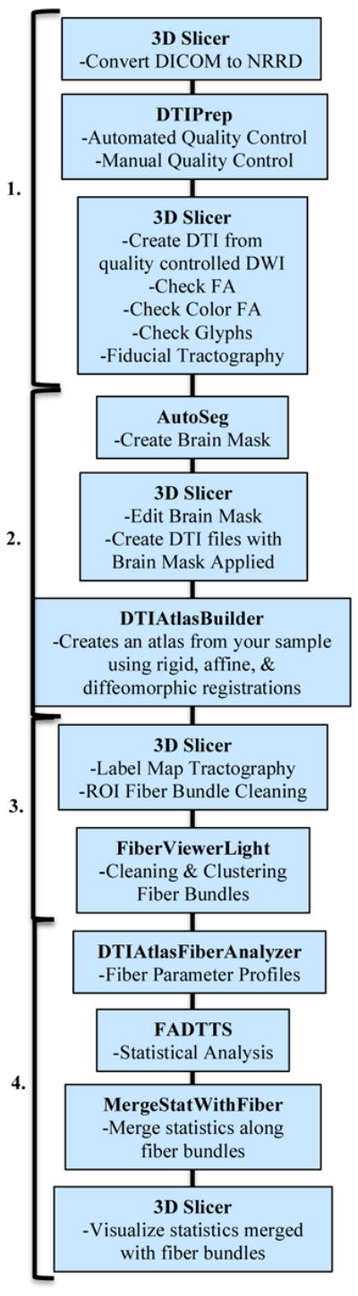
UNC-Utah NA-MIC DTI framework. Step 1 is Quality Control. Step 2 is Atlas Creation. Step 3 is Interactive Tractography. Step 4 is Parameter Profile Creation & Statistical Analysis.

Sec 3.1 Quality Control

The first step in our framework is the conversion of raw diffusion weighted images (DWI) from DICOM format to NRRD format through the use of 3D Slicer. This conversion tool is extensive in its support of multiple manufacturer specific tags, such as computing diffusion gradient information via the b-matrix stored within Siemens DICOM headers. Next, automatic DWI and DTI quality control will be performed using a tool called DTIPrep, which includes a variety of quality checks as well as eddy current and motion correction ^[3]. Visual QC is then performed to eliminate DWIs suffering from artifacts that were not picked up in the automated step (see Figure 2A). Furthermore, the overall quality of the resulting DTI data is assessed within 3D Slicer. First, the fractional anisotropy (FA) image quality is assessed regarding its apparent signal to noise ratio. Next, the color FA image is analyzed to determine that the major tracts are colored appropriately with red indicating tracts running left to right, green indicating tracts running in the anterior-posterior direction, and blue/purple indicating tracts running in the inferior-superior direction (Figure 2B). Glyph visualization as lines or ellipsoids allows you to verify the correctness of the diffusion measurement frame (see Figure 2C). If the glyphs are incorrect (due to incorrect DICOM information or scanner software issues), they will not follow the expected fiber tract “flow” and the measurement frame for the appropriate direction will need to be altered in the image header file. Next, investigative fiducial tractography is performed for selected tracts of interest; commonly the uncinate, the cingulum, the three portions of the corpus callosum (genu, midbody, and splenium), and the internal capsule. This rather coarse fiducial tractography is important to assess the expected normalcy of the tractography results (Figure 2D).

Figure 2.

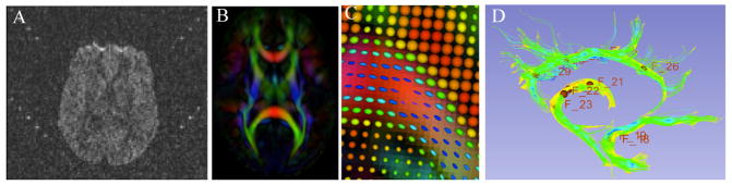
A. An example of a DWI artifact that would not be removed in the automated run of DTIPrep quality control (QC). This sort of artifact would be removed upon manual visual QC with DTIPrep. B. Color FA as visualized in 3D Slicer. C. A close up of the ellipsoid glyphs. As the FA becomes higher along tracts, the ellipsoids become more elongated and cooler in color. Low FA is indicated by round, red ellipsoids. D. An example of fiducial tractography QC in 3D Slicer showing tractography feasibility of the cingulum, fornix, and uncinate.

Sec 3.2 Atlas Building

The first step in atlas building is skull stripping. This can be achieved via various tools, such as the ‘Brain Mask from DWI’ module within Slicer or with a tool called AutoSeg^[4]. Mask editing is performed also within 3D Slicer, but any editing tools with Slicer compatible format (NRRD, Nifti, GIPL, Analyze) can be employed such as itk-SNAP^[5].

The edited brain mask can then be applied to the original DTI, creating skull stripped DTI images ready for atlas creation. Atlases are created iteratively starting from affine atlases (step 1) over deformable diffeomorphic atlases (step 2 and 3). All atlas registrations are performed via FA images intensity normalized to the current step’s atlas.

The main atlas building step is performed with a tool called DTIAtlasBuilder, detailed in Figure 3. This program allows the user to create an atlas image as an average of several registered DTI images. The registration is done in three steps: an affine registration with a module from the tool Brain Research: Analysis of Images, Networks, and Systems (BRAINS) called BRAINSFit^[6], a non-linear registration with the GreedyAtlas module within AtlasWerks^[7], and this is followed by a second non-linear registration with the tool DTI-Reg employing either BRAINSFit/BRAINSDemonWarp or Advanced Normalization Tools (ANTS). A final step will apply the transformations to the original DTI images so that the average can be computed to create the final DTI atlas.

Figure 3.

A. DTIAtlasBuilder tool workflow. Creating an atlas from your subjects with affine and diffeomorphic registration. B. DTIAtlasBuilder GUI. C. Progression from a single subject color FA, to the Final Affine Atlas, and then to the Final DTI Atlas using the pipeline shown in A.

In the first step, DTIAtlasBuilder will take all of FA images and affinely register them with the selected subject’s FA or with a reference template atlas, commonly in MNI-normative space. The output FA for each subject will then be averaged to create an intermediate affine atlas. This affine registration can be done in several loops. At each loop the normalization and the registration will be repeated with a new reference to improve the quality. The reference is the first FA image or a template that the user supplies for the first loop, and then an average is computed at the end of the loop. This FA average will be used as the template for the subsequent loop if multiple loops were indicated. The nonlinear or diffeomorphic atlas is the atlas computed from the affine registered FAs to get the deformation fields from the affine space to the non-linear atlas space through an unbiased diffeomorphic, fluid flow based atlas building within GreedyAtlas. These deformation fields will be applied to the original DTIs, which will be used to compute a deformably registered DTI average image, here termed the diffeomorphic atlas. The user can indicate the desired scale levels for GreedyAtlas and several options for the image resampling and the average image computation. The final resampling step, which creates the global deformation fields from the original space to the final atlas space, is done with DTI-Reg. DTI-Reg can call either BRAINSFit/BRAINSDemonWarp or ANTS with the options for each being fully modifiable. We generally recommend the use of ANTS which provides a significant boost in registration quality but also has an order of magnitude larger computation time costs.

Once the atlas computation is complete, quality control can be performed on the affine, diffeomorphic, and final resampled atlases using MriWatcher. With this quality control step we can visually determine the point to point correspondence between the subject images and the atlas to determine if computed registration transforms are appropriate. This final atlas is then utilized as an analysis coordinate and reference space, as well as for fiber tractography. The progression of atlas sharpness can be seen in Figure 3C.

Software path configuration for the tool can be performed automatically or manually, and the settings can be saved for future use. This tool also has a ‘no GUI’/command line option, given that data file, parameter file, and software configuration file are available (all can be determined and saved via the GUI). There is also direct support for the GRID software LSF (Load Sharing Facility, Platform Computing, Inc).

Sec 3.3 Tractography

While atlas building is fully automatic, the definition of fiber tracts of interest needs to be performed interactively. This fiber tractography only needs to be performed once, on the deformable atlas built in the prior step (Figure 4). In our framework, fiber tractography is performed via the label map tractography module or the full brain tractography module within 3D Slicer. Extracted DTI fiber bundles need to be post-processed to remove unwanted, erroneous fibers. This fiber cleaning is performed via interactive 3D regions of interest in 3D Slicer as well as a clustering based selection process in a tool called FiberViewerLight, which uses a number of pair-wise clustering metrics (fiber length, center of gravity, Hausdorff distance, mean distance and normalized cut) (Figure 5). Once fiber bundles are deemed appropriate, diffusion property profiles for each fiber tract and subject image are extracted as described in the next section.

Figure 4.

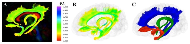
A. Cingulum, Uncinate, and Fornix tracts mapped on the Final DTI Atlas colored by FA. B. The same tracts shown in a glass brain model colored by FA. C. The same tracts colored by tract. Cingulum in blue, Fornix in green, and Uncinate in red.

Figure 5.

Shows the GUI for FiberViewerLight displaying the left uncinate. The two insets on the bottom right depict the left uncinate as viewed in the plane option. The red line in the left picture is actually a plane (as seen better in the right picture) that is manually placed to intersect the fiber bundle at 90 degrees to distinguish the origin for analysis in DTIAtlasFiberAnalyzer.

Sec 3.4 Property Profiles and Statistical Analysis

As a final step prior to statistical analysis, diffusion properties along the fiber tracts, called fiber property profiles, are extracted^[8]. For that purpose, a fiber tract parametrization needs to be established, which is achieved via arclength parameterization starting from each fiber’s intersection with an “origin” plane. While our tools automatically determine an appropriate origin plane, often investigators choose to interactively determine that plane in order to associate a specific anatomical fiber location to this origin. Origin plane creation can be achieved with FiberViewerLight (see Figure 5).

The parameter profile generation and processing is performed with a tool called DTIAtlasFiberAnalyzer, shown in Figure 6. The profile extraction operates on the original DTI data in order to avoid the need for tensor deformation by deforming the parametrized fibers into original space via the previously computed deformable transforms. At the deformed fiber locations the tool can then calculate the different fiber property profiles along each fiber in the bundle (FA, RD, AD, MD, GA, Fro, lambda 2, and lambda 3). See Figure 6 for an example origin plane created with FiberViewerLight and example FA profiles calculated and visualized with DTIAtlasFiberAnalyzer. From these fiber property profiles you can see how well the average of your subjects (thick tan line) matches the properties of the atlas (thick blue line), and how each of your subjects mapped into atlas space. This is an important quality control step assessing how well your subjects are mapped into your atlas and which subjects may be outliers.

Figure 6.

A. DTIAtlasFiberAnalyzer GUI; shown on the attribute tab. B. The inset to the right shows a visualization from the DTIAtlasFiberAnalyzer Plotting Parameters tab, showing FA profiles for the left uncinate. The left uncinate atlas FA profile is shown as a thick blue line, the average FA profile for the subjects with a thick tan line, and the individual subject FA profiles in green and red lines. The Arc length along the fiber in reference to the origin plane is shown on the x-axis, with zero indicating the origin. The FA along the fiber is displayed on the y-axis.

The fiber property profile outputs from DTIAtlasFiberAnalyzer are the inputs for the tool called Functional Analysis of Diffusion Tensor Tract Statistics (FADTTS) that performs statistical analysis on the fiber bundles^[9]. This tool has the ability to compute group difference and correlational analyses (Figure 7A). Currently the FADTTS tool is not incorporated into 3D Slicer but works through Matlab, and requires a Matlab familiar user to operate.

Figure 7.

A. FADTTS p-value plot for the left uncinate FA and four study covariates. The x-axis designates the location along the fiber in respect to the plane, where the plane is located at zero. The y-axis designates the −log of the p-value. B. Covariate p-values calculated with FADTTS (part A) merged onto the fiber with MergeStatWithFiber, and visualized in 3D Slicer. Here you see the left uncinate colored by the p-values of four different covariates. All points that are above the set significance threshold are colored royal blue. All points below the significance threshold are colored according to the level of significance. Significance coloration starts from light blue to red, with red representing the areas of greatest significance.

Once the statistics are computed, the results are merged back with the fiber bundles using a tool within DTIAtlasFiberAnalyzer called MergeStatWithFiber (the final tab of the GUI seen in Figure 6A). The result of this merge is then visualized in 3D Slicer (Figure 7B). The color map shown is determined by the significance threshold set in MergeStatWithFiber, as such that all points on the fiber that have a p-value above the significance threshold are colored blue, and all points with values below the significance threshold are colored from light blue to red, with points indicated in red signifying the areas of greatest significance. If desired, this color map can be altered within Slicer to another color table.

4. CONCLUSIONS

This framework has been tested and applied to several studies. Here, we illustrate our framework in a study of the uncinate, fornix, and cingulum in Nicotine Smoking and Non-Smoking individuals. Most of this framework utilizes tools that are available as modules within 3D Slicer with a graphical user interface (GUI) to make the execution of this workflow easier for non-technical investigators. This framework addresses the need in the field for a cohesive workflow in the preprocessing and analysis of DTI.

While all tools employed here are individually available online (see appendix below), a comprehensive package with all needed executables is available as download via the 3D Slicer extension manager (version 4.3 and above).

References

- 1.Smith SM, et al. Tract-based spatial statistics: voxelwise analysis of multi-subject diffusion data. Neuro Image. 2006;31(4):1487–505. doi: 10.1016/j.neuroimage.2006.02.024. [DOI] [PubMed] [Google Scholar]
- 2.Pieper SHM, Kikinis R. 3D SLICER. Proceedings of the 1st IEEE International Symposium on Biomedical Imaging: From Nano to Macro; 2004. pp. 632–635. [Google Scholar]
- 3.Liu ZWY, Gerig G, Gouttard S, Tao R, Fletcher T, Styner M. Quality Control of Diffusion Weighted Images. Proceedings of SPIE 2010; 2010. pp. 1–9. [DOI] [PMC free article] [PubMed] [Google Scholar]
- 4.Gouttard SSM, Joshi S, Smith RG, Hazlett HC, Gerig G. Subcortical Structure Segmentation using Probabilistic Atlas Priors. Medical Image Computing and Computer Assisted Intervention, 3D Segmentation in the Clinic: A grand Challenge. 2007:37–46. [Google Scholar]
- 5.Paul A, Yushkevich JP, Hazlett Heather Cody, Smith Rachel Gimpel, Ho Sean, Gee James C, Gerig Guido. User-guided 3D active contour segmentation of anatomical structures: Significantly improved efficiency and reliability. Neuroimage. 2006;31(3):1116–28. doi: 10.1016/j.neuroimage.2006.01.015. [DOI] [PubMed] [Google Scholar]
- 6.Johnson HGH, Williams K. BRAINSFit: mutual information registrations of whole-brain 3D images, using the insight toolkit. The Insight Journal. 2007 [Google Scholar]
- 7.(SCI), S.C.a.I.I. AtlasWerks: A set of high-performance tools for diffeomorphic 3D image registration and atlas building. Available from: http://www.sci.utah.edu/software.html.
- 8.Goodlett CB, et al. Group analysis of DTI fiber tract statistics with application to neurodevelopment. Neuro Image. 2009;45(1 Suppl):S133–42. doi: 10.1016/j.neuroimage.2008.10.060. [DOI] [PMC free article] [PubMed] [Google Scholar]
- 9.Zhu H, et al. FADTTS: functional analysis of diffusion tensor tract statistics. Neuro Image. 2011;56(3):1412–25. doi: 10.1016/j.neuroimage.2011.01.075. [DOI] [PMC free article] [PubMed] [Google Scholar]