

Abstract
Background
Bipolar disorder (BD) is one of the leading causes of disability worldwide. Patients are further disadvantaged by delays in accurate diagnosis ranging between 5 and 10 years. We applied Gaussian process classifiers (GPCs) to structural magnetic resonance imaging (sMRI) data to evaluate the feasibility of using pattern recognition techniques for the diagnostic classification of patients with BD.
Method
GPCs were applied to gray (GM) and white matter (WM) sMRI data derived from two independent samples of patients with BD (cohort 1: n = 26; cohort 2: n = 14). Within each cohort patients were matched on age, sex and IQ to an equal number of healthy controls.
Results
The diagnostic accuracy of the GPC for GM was 73% in cohort 1 and 72% in cohort 2; the sensitivity and specificity of the GM classification were respectively 69% and 77% in cohort 1 and 64% and 99% in cohort 2. The diagnostic accuracy of the GPC for WM was 69% in cohort 1 and 78% in cohort 2; the sensitivity and specificity of the WM classification were both 69% in cohort 1 and 71% and 86% respectively in cohort 2. In both samples, GM and WM clusters discriminating between patients and controls were localized within cortical and subcortical structures implicated in BD.
Conclusions
Our results demonstrate the predictive value of neuroanatomical data in discriminating patients with BD from healthy individuals. The overlap between discriminative networks and regions implicated in the pathophysiology of BD supports the biological plausibility of the classifiers.
Key words: Bipolar disorder, diagnosis, Gaussian process classifiers, imaging, pattern recognition
Introduction
Bipolar disorder (BD) is a complex psychiatric disorder characterized by severe mood dysregulation (APA, 1994). BD is associated with significant psychosocial morbidity and mortality (Angst et al. 2002; Baldessarini & Tondo, 2003) and is among the leading causes of disability worldwide (WHO, 2004). Despite illness severity, the delay between onset and accurate diagnosis is typically between 5 and 10 years (Lish et al. 1994; Hirschfeld et al. 2003; Berk et al. 2007). Surveys of BD patients conducted over the past 20 years show no evidence of improvement in timely illness recognition (Hirschfeld et al. 2003; WHO, 2004; Berk et al. 2007). Delayed diagnosis in BD has adverse consequences in terms of increased periods in episode, greater psychosocial morbidity (Stensland et al. 2008) and emerging treatment resistance (Post et al. 2003; Ketter et al. 2006). Delayed diagnosis is also associated with increased treatment costs (Stensland et al. 2008) whereas early and accurate identification of BD leads to significant cost savings (Menzin et al. 2009). The importance of early recognition in BD is further underscored by emerging yet compelling evidence that the illness is associated with evolving neurobiological changes that may drive subsequent clinical deterioration (Berk et al. 2009; Kapczinski et al. 2009). Therefore, the timely diagnosis of BD is currently the single most important unmet need in enhancing clinical and functional outcomes.
Neuroimaging studies to date have established that structural magnetic resonance imaging (sMRI) can be used to identify brain morphological differences between BD patients and controls. Meta-analytic studies that have synthesized the extensive available literature have confirmed that BD is reliably associated with structural abnormalities in the ventral prefrontal cortex, the cingulate gyrus, amygdala/parahippocampal complex and the basal ganglia (Kempton et al. 2008; Arnone et al. 2009; Vita et al. 2009; Bora et al. 2010; Ellison-Wright & Bullmore, 2010; Kempton et al. 2011; Selvaraj et al. 2012). Despite the contribution of these findings to our understanding of the pathophysiology of BD, their clinical usefulness has been negligible. This is primarily because conventional sMRI data analyses compute mean group differences in spatial localized anatomical regions and do not make use of information about the distributed pattern of relationships among regions or voxels. Information about these spatial patterns is of particular relevance as it can be used for the diagnostic classification of individual patients, thus bridging the gap between neuroscience and clinical practice. In this respect, recent advances in multivariate pattern recognition techniques represent a major development.
The most commonly used pattern recognition algorithm has been the support vector machine (SVM) classifier. The SVM classifier has been used for the classification of patients with Alzheimer's disease (Klöppel et al. 2008; Vemuri et al. 2008), autism (Ecker et al. 2010), aphasia (Wilson et al. 2009) and psychosis (Koutsouleris et al. 2009; Mourao-Miranda et al. 2012) and to predict clinical variables based on patterns of brain activation in functional MRI (Fu et al. 2008; Marquand et al. 2008). However, the SVM classifier yields binary (case or control) and not probabilistic outcomes. For many applications, probabilistic predictions are desirable as they have two key advantages: they provide accurate quantification of predictive uncertainty, reflecting variability within subject groups (e.g. in quantifying the probability that a subject has a psychiatric disorder within a population where illness severity can be expected to vary between individuals), and they allow adjustment of predictions to compensate for different frequencies of diagnostic classes within the general population (Bishop, 2006). Gaussian process classifiers (GPCs) represent a significant advance over SVM as they are fully probabilistic pattern recognition models based on Bayesian probability theory. For neuroimaging, GPCs combine equivalent predictive performance to SVM with the additional benefit of probabilistic classification (Marquand et al. 2010).
Therefore, we used GPCs to examine the predictive value of whole-brain gray (GM) and white matter (WM) anatomy in discriminating patients with BD from healthy individuals. We embedded the classifier in a recursive feature elimination (RFE) framework (Guyon et al. 2002; Marquand et al. 2011) to identify and localize the subset of brain voxels that provide optimal discrimination accuracy. We focused on sMRI, rather than other neuroimaging techniques, as it is widely available, safe and has an established role in the diagnosis and management of brain disorders. Thus, a diagnostic aid based on sMRI data could be easily incorporated into routine clinical practice and is likely to have high patient acceptability. We enrolled patients with bipolar disorder, type 1 (BP-I; APA, 1994), whose diagnosis was further confirmed following detailed clinical assessment. Patients were in remission, free of any other lifetime psychiatric co-morbidity and matched to healthy controls on age, sex and general intellectual ability (IQ). This careful sample selection was designed to maximize the probability that discrimination between patients and controls would be attributable to brain structural changes relating to BD rather than other factors such as co-morbidity or general cognitive ability. Furthermore, we included two independent cohorts of patients and controls to determine the reliability of our findings.
Method
Samples
Cohort 1 comprised 26 patients fulfilling criteria for BP-I according to DSM-IV criteria (APA, 1994) and 26 healthy controls derived from participants in the Maudsley Bipolar Disorder Project (Frangou, 2005; Frangou et al. 2005). Demographic and clinical information on the sample is shown in Table 1. Nineteen BD patients were prescribed psychotropic medications, often in combination (typical antipsychotics = 4, atypical antipsychotics = 4, lithium = 10, carbamazepine = 7, sodium valproate = 2). None of the patients were prescribed benzodiazepines, anticholinergics or any other medication.
Table 1.
Demographic and clinical characteristics of the study samples
| Cohort 1 | Cohort 2 | |||
|---|---|---|---|---|
| Patients with BD (n = 26) | Healthy controls (n = 26) | Patients with BD (n = 14) | Healthy controls (n = 14) | |
| Age (years) | 41.5 (11.27) | 41.3 (11.65) | 37.6 (11.97) | 37.4 (10.98) |
| Male:Female | 12:14 | 12:14 | 6:8 | 6:8 |
| IQ | 102.3 (15.93) | 103.3 (17.37) | 108.6 (16.88) | 110.9 (18.99) |
| Age of onset (years) | 25.7 (9.22) | – | 18.8 (7.43) | – |
| HAMD | 6.6 (3.39) | – | 4.2 (5.15) | – |
| MRS | 1.8 (4.11) | – | 1.7 (3.12) | – |
| GAF | 71.1 (11.31) | – | 70.2 (24.14) | – |
BD, Bipolar disorder; HAMD, Hamilton Depression Rating Scale; MRS, Mania Rating Scale; GAF, Global Assessment of Functioning.
Continuous data expressed as mean (standard deviation).
Cohort 2 comprised 14 patients fulfilling DSM-IV criteria for BP-I and 14 healthy controls derived from participants in the Vulnerability Indicators to Bipolar Disorder Study (VIBES; Frangou, 2009). Demographic and clinical information on the sample is shown in Table 1. All patients in this sample were on treatment with anticonvulsant (sodium valproate = 10, carbamazepine = 4) monotherapy and did not receive any other type of medication.
For both samples, patients had an established diagnosis of BD and were receiving out-patient treatment within secondary care services. They were individually matched on sex, age and IQ to an equal number of healthy controls without a personal or family history of any DSM-IV Axis I disorders. All participants were screened to exclude past, current and hereditary neurological disorders, current medical conditions, DSM-IV current or lifetime drug or alcohol dependence or abuse, and other DSM-IV Axis I current or lifetime co-morbidity and contraindications to MR imaging. All participants were assessed by qualified psychiatrists using the Structured Clinical Interview for DSM-IV for Axis I Disorders, Patient or Non-Patient Version (SCID-I/P and SCID-I/NP; First et al. 2002a,b) and the Family Interview for Genetic Studies (FIGS; Maxwell, 1992), with additional information supplemented by medical notes as appropriate. Psychopathology was assessed using the Hamilton Depression Rating Scale (HAMD; Hamilton, 1960) and the Mania Rating Scale (MRS; Spitzer & Endicott, 1978), and psychosocial functioning was assessed with the Global Assessment of Functioning (GAF) scale (APA, 1994). Patients were scanned when in remission operationalized as (a) the absence of syndromal episode for ⩾3 months, (b) being prescribed the same type and dose of medication for ⩾3 months, and (c) having HAMD and MRS total scores of <10 on the day of scanning. An estimate of general intellectual ability was obtained using the National Adult Reading Test (NART; Nelson & Wilson, 1992). Patients in cohort 2 were younger, had an earlier age of onset and higher IQ than those in cohort 1 (p < 0.01).
This study was approved by the Joint Ethics Committee of the Institute of Psychiatry and the South London and Maudsley National Health Service (NHS) Foundation Trust. Written informed consent was obtained from all participants after a detailed description of the study.
MRI data acquisition
Participants were scanned using a 1.5-T GE NV/i Signa MR system (GE Medical Systems, USA) at the Maudsley Hospital, London. The whole brain was imaged with a three-dimensional (3D) inversion recovery prepared fast spoiled gradient-recalled acquisition in the steady state (SPGR) T1-weighted dataset. These T1-weighted images were obtained in the axial plane with 1.5-mm contiguous sections (echo time = 5.1 ms, repetition time = 18 ms, flip angle = 20°, slice thickness = 1.5 mm, in-plane resolution = 0.9375 × 0.9375 mm, number of excitations = 1). Image contrast for all datasets was chosen with the aid of optimizing software (Simmons et al. 1996).
Data preprocessing
For both samples, all images were first visually inspected for artifacts or gross structural abnormalities using criteria described previously (Simmons et al. 1996, 2011). Subsequently, images were preprocessed using SPM5 (www.fil.ion.ucl.ac.uk/spm/software/spm5). Using the unified segmentation step included in SPM5, images were normalized and segmented (Ashburner & Friston, 2005). Normalized and modulated GM and WM segmented images were then smoothed with 8-mm isotropic Gaussian kernels and used as input into the classification algorithms.
Pattern classification analysis
The probability of group membership was determined separately in each cohort using GPCs to the MRI data. Technical descriptions of GPC inference have been presented elsewhere (Bishop, 2006; Rasmussen & Williams, 2006; Marquand et al. 2008, 2010) and are summarized in the online Supplementary Material. In brief, the classifier is first trained to determine a predictive distribution that best distinguishes cases from controls; any parameters controlling the behavior of this distribution are computed by maximizing the logarithm of the marginal likelihood on the training data only. Then, in the test phase, the classifier predicts the group membership of a previously unseen example. This is achieved by integrating over the predictive distribution for the test case and passing the output through a sigmoidal function, resulting in predictive probabilities scaled between 0 and 1 that precisely quantify the predictive uncertainty of the classifier for the test case.
In each cohort, the GPCs for GM and WM were implemented separately in the PROBID software package (http://www.kcl.ac.uk/iop/depts/neuroimaging/research/imaginganalysis/Software/PROBID.aspx). We embedded each classifier in a recursive feature elimination (RFE) framework (Guyon et al. 2002; Marquand et al. 2011), which enabled us to identify the subset of brain voxels that provided the optimal discrimination accuracy and to accurately localize the most discriminative brain voxels. To achieve this, we used nested (three-way) cross-validation where we first excluded a matched pair of subjects (one from each group) to comprise the test set, and then performed a second split where we repeatedly repartitioned the remaining subject pairs into a validation and a training set. We then repeatedly trained the classifier on the training set, removing a subset of the least informative features at each iteration, until no features remained. We used a common ranking criterion based on the GPC predictive weights to quantify the information content of each voxel at each iteration (Marquand et al. 2011) and used a small step size (∼1% of voxels) to provide fine-grained control over the number of features retained. In each case we selected the number of features that produced maximal accuracy on the validation set before applying it to the test set. We thresholded the probabilistic predictions at 0.5 to convert the probabilistic predictions to class labels and computed the proportion of subjects having the correct label across all test splits to estimate the classification accuracy. The statistical significance of each classifier was determined by permutation testing. This test was used to derive a p value to determine whether the classification accuracy exceeded chance levels (50%). To achieve this, we permuted the class labels from the training set 1000 times (i.e. each time randomly assigning class labels to each structural MRI pattern) and repeated the entire RFE procedure. We then counted the number of times the permuted test accuracy was equal to or greater than the one obtained for the true labels. Dividing this number by 1000, we derived a p value of the classification accuracy.
Cross-validation
The performance of the GM and WM classifiers for each cohort separately was estimated in four ways. First, for each classifier within each sample we computed the proportion of images correctly classified as BD patients or controls (i.e. classification accuracy). Second, we quantified the sensitivity and specificity of each classifier defined as: sensitivity = TP/(TP + FN) and specificity = TN/(TN + FP), where TP is the number of true positives (number of images of patients correctly classified), TN is the number of true negatives (number of images of controls correctly classified), FP is the number of false positives (number of images of controls classified as patients) and FN is the number of false negatives (number of images of patients classified as controls). Third, we compared the results obtained through the GPCs to those derived from conventional univariate voxel-based morphometry (VBM) implemented in SPM5. In VBM analyses we used a statistical threshold of p < 0.0001 uncorrected for multiple comparisons. Thus we preserve a reasonable degree of specificity in favor of increased sensitivity as the aim of this analysis was to assist in making inferences about the contribution of different regions to the spatially distributed pattern associated with a diagnosis of BD. This is in contrast to the more stringent inferential methods used for controlling type I error to find highly localized, spatially segregated focal group differences. Fourth, regression analyses, thresholded at p < 0.001 uncorrected, were implemented in SPM5 using cumulative exposure to lithium or antipsychotics (based on doses transformed to chlorpromazine equivalents) to identify potential effects of medication on the GM and WM volumes of patients.
GPC discrimination maps
The discrimination map (Rasmussen & Williams, 2006) is a spatial representation of the vector of GPC predictive weights and describes the relative contribution of each brain voxel to the classifier decision. Technical details of GPC discrimination mapping have been published elsewhere (Bishop, 2006; Marquand et al. 2010) and are described in the online Supplementary Material. The process is illustrated in Fig. 1 based on a simplified hypothetical example of a two-voxel image.
Fig. 1.
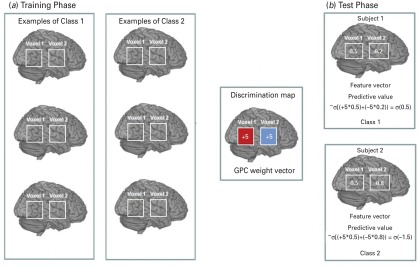
A hypothetical example based on a simplified version of the Gaussian process classifier (GPC) decision function considering two gray matter (GM) voxels per image.
To provide an intuitive interpretation of the maps, we consider a simplified version of the GPC decision function. The class probability p is given by ply = class 11 x, w) = o(xt wI, where y is the class label of a test subject (if y > 05 corresponds to class 1, otherwise it corresponds to class 2), x is the feature vector containing gray matter voxels for the test subject, wis referred to as the maximum a posteriori estimate of the GPC weight vector, and is the best point estimate of the GPC decision function (i.e. the mode of the Gaussian approximation in voxel space) and a is a sigmoid function that maps the values to the interval [0,1). (A) Training phase: Through training the GPC classifier assigns for each voxel a weight value w = (+5, −5); +5 represents a voxel containing predictive contribution for class 1 displayed in red and −5 represents a voxel containing predictive contribution for class 2 (displayed in blue). (S)Test Phase: The feature vector (vector containing gray matter probability assigned for each voxel) is shown within each of the two voxels in the two-voxel image example. During the test phase, for classifying a new example we first mUltiplied each voxel by its corresponding coefficient in the weight vector. After that we add all multiplied values and pass the sum through a sigmoid function in order to obtain an output (i.e. predictive probabilities) between 0 and 1. In the illustrative eKample above: Subject 1: The feature vector for this subject is (0.5, 0.2). The predictive value for this subject is 0[(+5*0.5) + (−5*0.2)) = 0(0.5) which corresponds to a predictive probability above 0.5. Therefore subject 1 will be classified as class 1. For the subject 1, a low value in the voxel 2, which has negative coefficient in the weightvector, contributed to the classification of this subject as class 1. Subject 2: The feature vector for this subject is (0.5, 0.8). The predictive value for this subject is 0[(+5*0.5) + (−5*0.8)) = 0(−1.5) which corresponds to a predictive probability below 0.5. Therefore subject 2 will be classified as class 2. For subject 2, a high value in the voxel2, which has a positive coefficient in the weight vector, contributesto the classification ofthis subject as class 2.
Results
Prediction accuracy
Classification accuracy reflects the predictive power of the algorithm and is therefore of direct diagnostic relevance. For cohort 1, classification accuracy using GPC analysis of GM images was 73% with a sensitivity and specificity of 77% and 69% respectively. In other words, based on a GM anatomical scan, if a participant had a clinical diagnosis of BD, the probability of correct classification was 0.77. Conversely, if a participant did not have BD, the probability of being correctly classified as a control was 0.69. The GPC analysis using WM images for cohort 1 yielded an accuracy of 69% with a sensitivity of 69% and specificity of 69%. For cohort 2, the sensitivity and specificity of the GM classification were 64% and 99% respectively and the overall accuracy was 72%. In the same cohort, GPC analysis using WM images yielded an accuracy of 78% with a sensitivity of 71% and specificity of 86%. For both cohorts, the models were significant at p < 0.001.
Discrimination maps
Discrimination maps showing the global spatial pattern by which the groups differ are illustrated in Fig. 2 and detailed in Tables 2 (GM) and 3 (WM) for cohort 1 and in Fig. 3 and Tables 4 (GM) and 5 (WM) for cohort 2. For both cohorts, the maps highlight those regions that, according to our GPC-RFE classification approach, contain the most discriminating voxels between BD patients and controls. This optimal discriminative pattern was obtained following removal of ∼98% of all voxels. Because of the multivariate character of the GPC, the discrimination maps should not be interpreted as describing focal effects within individual brain regions. Instead they represent a spatially distributed pattern of coefficients that quantify the contribution of each voxel to the GPC decision function (i.e. the value of a voxel in the discrimination map reflects its contribution or predictive value towards one class or the other). We used the following convention: class 1 was the BD group, with labels +1, and class 2 was the control group, with labels −1. In the discrimination map, positive coefficients indicate voxels with a predictive value for BD (class 1; visualized in red color scale) and negative coefficients indicate voxels with a predictive value for controls (class 2; visualized in blue color scale); by definition, a voxel with negative predictive weight for patients has the same positive predictive weight for controls.
Fig. 2.
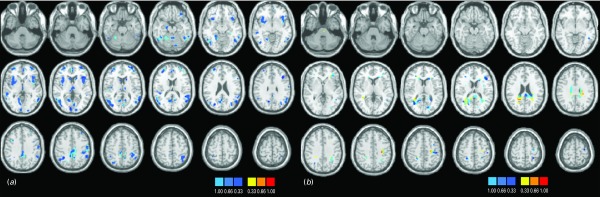
Discrimination maps for (a) gray matter (GM) and (b) white matter (WM) classification in cohort 1.
Table 2.
Cohort 1: gray matter (GM) regions discriminating between individuals with bipolar disorder (BD) and controls
| Region | Laterality | BA | Coordinates | Cluster sizea | Wi b | ||
|---|---|---|---|---|---|---|---|
| x | y | z | |||||
| Frontal lobe | |||||||
| Middle frontal gyrus | R | 10 | 33.3 | 49.9 | 11.7 | 466 | −16.7 |
| L | 10 | −31.6 | 55.3 | 7.7 | 397 | −16.6 | |
| 9 | −39 | 23.9 | 27.7 | 93 | −21.8 | ||
| Inferior frontal gyrus | L | 11 | −30.6 | 35.8 | −16.9 | 71 | −14.0 |
| Parietal lobe | |||||||
| Inferior parietal lobule | R | 40 | 39.6 | −54 | 41 | 221 | −22.4 |
| L | 40 | −43.1 | −35.8 | 44.5 | 569 | −16.8 | |
| Temporal lobe | |||||||
| Superior temporal gyrus | R | 41 | 48.1 | −32.1 | 15.2 | 76 | −14.5 |
| L | 39 | −52.8 | −55.4 | 23.5 | 832 | −18.4 | |
| Fusiform gyrus | L | 37 | −45.7 | −59.7 | −14.7 | 210 | −16.1 |
| Middle temporal gyrus | R | 21 | 57.3 | −37.8 | −2.4 | 155 | −13.6 |
| L | 37 | −56.6 | −54.1 | −8.9 | 204 | −16.3 | |
| Occipital lobe | |||||||
| Lingual gyrus | R | 19 | 33.3 | −63.1 | 2.7 | 1759 | −18.2 |
| 17 | 7.2 | −94.1 | 2.9 | 111 | −18.0 | ||
| Cuneus | L | 18 | −4.3 | −76.4 | 6.3 | 109 | −10.0 |
| Superior occipital gyrus | L | 19 | −31.6 | −72.9 | 26.4 | 84 | −15.6 |
| Middle occipital gyrus | R | 19 | 29 | −76.3 | 24.2 | 53 | −18.0 |
| Limbic lobe | |||||||
| Parahippocampal gyrus | R | 28 | 20.8 | −14.6 | −19.6 | 55 | −12.8 |
| Anterior cingulate gyrus | L | 32 | −0.4 | 48.8 | 5.55 | 179 | −11.7 |
| Posterior cingulate gyrus | R | 31 | 0.4 | −37.9 | 40.4 | 759 | −12.2 |
| 30 | −9.5 | −60.4 | 12.2 | 71 | −9.2 | ||
| Insula | R | 13 | 34.7 | 9.6 | 2.2 | 707 | −14.1 |
| L | 13 | −38.7 | 16.2 | −1.4 | 747 | −15.5 | |
| Thalamus | L | – | 0 | −18.1 | 6 | 184 | −14.6 |
| Striatum | |||||||
| Caudate | R | – | 11 | 15.7 | 5.7 | 50 | −12.2 |
| L | – | 7 | 16.9 | 6.7 | 77 | –16.1 | |
| Cerebellum | L | – | 20.8 | −61.4 | −53.4 | 582 | −16.2 |
| R | – | −28.9 | −66.3 | −52.6 | 257 | −12.5 | |
BA, Brodmann area; R, right; L, left.
Coordinates are shown in Montreal Neurological Institute (MNI) standard space; x = sagittal, y = coronal, z = axial.
Number of voxels.
Highest weights within individual clusters.
Table 3.
Cohort 1: white matter (WM) regions discriminating between individuals with bipolar disorder (BD) and controls
| Region | Laterality | Coordinates | Cluster sizea | Wi b | ||
|---|---|---|---|---|---|---|
| x | y | z | ||||
| Frontal lobe | ||||||
| Inferior frontal gyrus | L | −46 | 25 | 17 | 110 | −55.8 |
| Parietal lobe | ||||||
| Inferior parietal lobule | L | −46 | −27 | 51 | 363 | −44.2 |
| −34 | −41 | 39 | 186 | −30.1 | ||
| Precuneus | R | 28 | −47 | 51 | 156 | −44.4 |
| Postcentral gyrus | L | −26 | −23 | 41 | 133 | 28.1 |
| Supramarginal gyrus | L | −26 | −29 | 29 | 231 | 21.1 |
| Occipital lobe | ||||||
| Middle occipital gyrus | L | −50 | −55 | 7 | 66 | −43.2 |
| R | 36 | −67 | 13 | 1156 | −48.9 | |
| Cuneus | L | −12 | −79 | 13 | 87 | −25.8 |
| Precuneus | L | 20 | −49 | 25 | 441 | 23.3 |
| Limbic lobe | ||||||
| Cingulate gyrus | L | −2 | −35 | 23 | 832 | −35.2 |
| Corpus callosum | ||||||
| Genu | R | 16 | 25 | 9 | 83 | −19.9 |
L, Left; R, right.
Coordinates are shown in Montreal Neurological Institute (MNI) standard space; x = sagittal, y = coronal, z = axial.
Number of voxels.
Highest weights within individual clusters.
Fig. 3.
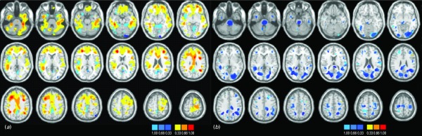
Discrimination maps for (a) gray matter (GM) and (b) white matter (WM) classification in cohort 2.
Table 4.
Cohort 2: gray matter (GM) regions discriminating between individuals with bipolar disorder (BD) and controls
| Region | Laterality | BA | Coordinates | Cluster sizea | Wi b | ||
|---|---|---|---|---|---|---|---|
| x | y | z | |||||
| Frontal lobe | |||||||
| Middle frontal gyrus | R | 10 | 28.0 | 41.0 | 17.0 | 650 | 14.369 |
| Parietal lobe | |||||||
| Inferior parietal lobe | L | 7 | −42.0 | −69.0 | 47.0 | 49 | −11.18 |
| Temporal lobe | |||||||
| Middle temporal gyrus | L | 39 | −44.0 | −65.0 | 17.0 | 29 | −73.482 |
| Occipital lobe | |||||||
| Middle occipital gyrus | L | 18 | −30.0 | −83.0 | −7.0 | 245 | 64.639 |
| 19 | −30.0 | −91.0 | 7.0 | 32 | −92.226 | ||
| R | 18 | 24.0 | −89.0 | 11.0 | 17 | −10.218 | |
| Inferior occipital gyrus | R | 18 | 26.0 | −91.0 | −7.0 | 184 | 34.588 |
| Lingual gyrus | L | 17 | −14.0 | −97.0 | −17.0 | 193 | −11.478 |
| R | 17 | 10.0 | −95.0 | −17.0 | 25 | −19.075 | |
| Cuneus | R | 23 | 12.0 | −71.0 | 9.0 | 90 | −21.117 |
| Limbic lobe | |||||||
| Anterior cingulate gyrus | L | 32 | −3.0 | 42.0 | 7.0 | 650 | 12.45 |
| R | 32 | 5.0 | 40.0 | 6.0 | 650 | 12.19 | |
| Thalamus | L | – | −6.0 | −11.0 | 5.0 | 69 | 21.513 |
| Cerebellum | R | – | 28.0 | −87.0 | −39.0 | 9 | −0.753 |
BA, Brodmann area; R, right; L, left.
Coordinates are shown in Montreal Neurological Institute (MNI) standard space; x = sagittal, y = coronal, z = axial.
Number of voxels.
Highest weights within individual clusters.
There is significant overlap between the cohorts. In terms of GM, regions within the frontopolar and ventral prefrontal cortex, the parietal lobules, the middle/superior temporal gyri, the lingual gyrus and cuneus and within the thalamus and cerebellum emerge as being implicated most consistently in the diagnosis of BD. A similar conclusion can be drawn for WM tracts traversing ventral prefrontal regions, parietal and postcentral regions, the middle occipital gyrus and the cuneus, the cingulum and genu of the corpus callosum. Discriminative regions were more extensive in cohort 2, which consisted of younger and less medicated patients than cohort 1, suggesting that the results of the GPCs are not driven by medication or age.
VBM
At the threshold of p < 0.0001 uncorrected, GM and WM volumetric differences between patients and controls were noted in multiple brain regions in both cohorts. Details of the regional maxima are provided in Supplementary Tables S1–S4. As discussed, the output of the GPC and VBM analyses are not directly comparable as the former reflects the predictive value of voxels in discriminating between patients and controls whereas the latter represents the mean differences between patients and controls. Nevertheless, there is significant overlap between the two outputs and between cohorts. An effect of medication was identified only in cohort 1, with cumulative lithium exposure being positively associated with the right anterior cingulate GM volume (x = 5.2, y = 41.1, z = 4, cluster size = 85). No correlations with medication dose were noted in cohort 2.
Discussion
To our knowledge, this is the first study to evaluate the feasibility of using pattern recognition algorithms for the automatic classification of sMRI data of patients with BD and healthy controls. We found that GPCs applied to GM reliably achieved above chance discriminative power solely on the basis of anatomical data, with classification accuracy ranging between 69% and 78%.
Prediction accuracy of GPCs applied to sMRI in BD
Neuroanatomical studies using conventional analyses have established the presence of morphological changes in BD (Kempton et al. 2008; Arnone et al. 2009; Vita et al. 2009; Bora et al. 2010; Ellison-Wright & Bullmore, 2010; Kempton et al. 2011; Selvaraj et al. 2012). However, these findings have had limited translational application primarily for three reasons: (a) there is considerable between-group overlap in brain morphological variables derived from group-level neuroimaging analyses (Kempton et al. 2008, 2009, 2011), (b) voxel-based analysis methods are significantly biased toward detecting group differences that are highly localized in space but are limited in detecting group differences that are spatially distributed and subtle (Davatzikos, 2004), and (c) voxel-based analyses do not lend themselves to making predictions at the level of individual subjects.
The data presented here demonstrate that these limitations may be surmounted with the aid of multivariate pattern recognition techniques. The application of GPC analysis to anatomical scans in BD provided diagnostic accuracy in the range 69–78%. As with any new test, the accuracy of the GPC classification for BD was determined against ‘gold standard’ diagnostic assessments. In this study ‘true positive cases’ (i.e. patients with BD) were identified using the SCID-I, conducted by clinicians with expertise in mood disorders. The SCID-I is designed to elicit the presence or absence of the operational criteria that define the syndrome of BD itself and is therefore expected to have the highest diagnostic accuracy (Williams et al. 1992; Fennig et al. 1994; Segal et al. 1994). A more appropriate comparison would be with behavior-based case-finding instruments, whose sensitivity and specificity are about 70%, such as the Mood Disorder Questionnaire (MDQ; Hirschfeld et al. 2000; Hirschfeld, 2010; Zimmerman et al. 2011). However, even more important is the comparison of our results to ‘real world’ clinical assessments where BD is either missed or misdiagnosed resulting in nearly a third of patients having to wait for approximately 10 years before they receive an accurate diagnosis (Lish et al. 1994; Hirschfeld et al. 2003; Berk et al. 2007). This is because of the substantial overlap between clinical symptoms of BD and those of other disorders, particularly major depressive disorder (MDD) because depressive symptoms are commonly present at onset (Perugi et al. 2000) and often dominate the clinical picture thereafter (Judd et al. 2002). Additionally, the presence of psychosis during manic or depressive episodes often leads to difficulties in distinguishing BD from schizophrenia and schizo-affective disorder (Schimmelmann et al. 2005). Further diagnostic challenges arise from the high level of co-morbidity of BD with other disorders, particularly substance abuse and anxiety disorders (McElroy et al. 2001; Merikangas et al. 2011). In this context, a classifier that is trained to identify true positives BD cases might have an important role in assisting clinicians when used in combination with other clinical measures.
The results presented here for the predictive value of sMRI data in BD compare favorably with classification accuracies of approximately 80% reported for Alzheimer's disease and schizophrenia, even though the magnitude of neuroanatomical deviance is greater for these disorders (reviewed by Klöppel et al. 2012).
Brain regions discriminating patients with BD from controls
The GM and WM discriminative maps generated by the GPCs show that clusters contributing to the distinction between BD patients and healthy controls are spatially distributed within cortical and subcortical regions (Tables 2–5). GM discriminative clusters consistently associated with BD in both cohorts were localized primarily within the frontopolar and ventral prefrontal cortex, the inferior parietal lobule, the medial and lateral temporal cortex, the cingulate cortex, occipital regions in the lingual gyrus and cuneus, the thalamus and cerebellum. This is in keeping with previous morphometric studies that have repeatedly shown an association between volumetric changes in these regions and disease expression for BD (Kempton et al. 2008, 2009, 2011; Scherk et al. 2008; Arnone et al. 2009; Yu et al. 2010; Hallahan et al. 2011). Previous research on global (Scherk et al. 2008; Vita et al. 2009) and regional (McIntosh et al. 2005; Stanfield et al. 2009) WM volume changes in BD yielded variable results. However, there is increasing consensus for an association between disease expression for BD and WM pathology within the cingulum (Vederine et al. 2011) and the genu of the corpus callosum (Bellani et al. 2009; Walterfang et al. 2009a,b; Bearden et al. 2011). Our findings in both cohorts suggest that WM regions of predictive value for BD patients are widespread but consistently include the cingulum and genu. Although the results of the VBM and GPC analyses cannot be compared directly, they showed significant overlap in terms of the spatial distribution of regions influenced by the diagnosis of BD.
Table 5.
Cohort 2: white matter (WM) regions discriminating between individuals with bipolar disorder (BD) and controls
| Region | Laterality | Coordinates | Cluster sizea | Wib | ||
|---|---|---|---|---|---|---|
| x | y | z | ||||
| Frontal lobe | ||||||
| Medial frontal gyrus | R | 2 | −19 | 66 | 415 | −89.186 |
| 21 | 39 | 25 | 154 | −64.624 | ||
| L | −34 | 34 | 26 | 366 | −86.983 | |
| Inferior frontal gyrus | R | 40 | 37 | −0 | 124 | −75.911 |
| L | −50 | 8 | 14 | 97 | −77.191 | |
| Middle frontal gyrus | R | 31 | 39 | 17 | 147 | −97.775 |
| 28 | 20 | 40 | 126 | −92.977 | ||
| L | −18 | 17 | 40 | 171 | −65.687 | |
| Parietal lobe | ||||||
| Postcentral gyrus | L | −54 | −19 | 19 | 413 | −74.915 |
| Precuneus | R | 20 | −59 | 49 | 313 | −10.468 |
| Superior parietal lobule | R | 22 | −43 | 56 | 311 | −42.827 |
| Temporal lobe | ||||||
| Middle temporal gyrus | R | 42 | −0 | −31 | 160 | −89.324 |
| Fusiform gyrus | L | −50 | −24 | −26 | 120 | −69.773 |
| Inferior temporal gyrus | R | 54 | −46 | −12 | 119 | −38.803 |
| Occipital lobe | ||||||
| Middle occipital gyrus | L | −27 | −71 | 14 | 574 | −13.083 |
| Inferior occipital gyrus | R | 27 | −93 | −8 | 285 | −93.779 |
| Cuneus | R | 28 | −65 | 12 | 338 | −11.814 |
| Limbic lobe | ||||||
| Cingulate gyrus | L | −2 | −36 | 27 | 966 | −10.604 |
| Corpus callosum | ||||||
| Genu | L | −9 | 29 | 14 | 26 | −44.234 |
| Cerebellum | R | 10 | −60 | −31 | 121 | −52.074 |
R, Right; L, left.
Coordinates are shown in Montreal Neurological Institute (MNI) standard space; x = sagittal, y = coronal, z = axial.
Number of voxels.
Highest weights within individual clusters.
Methodological considerations and future directions
In cohort 1, the majority of BD patients were medicated with antipsychotic or mood-stabilizing medication or both. Treatment with lithium has been associated with volumetric changes in BD, and specifically increases in global and regional volumes (Bearden et al. 2007; Kempton et al. 2008, 2009; Phillips et al. 2008; Germana et al. 2010; van Erp et al. 2012). In line with this, we observed a positive association between lithium dose and GM volume in the anterior cingulate in cohort 1. However, medication effects related to lithium or antipsychotics cannot fully explain the results because patients in cohort 2 were not on these medications.
The GPCs were trained to segregate healthy controls from patients with BD. This represents the necessary first step in developing pattern recognition approaches for use as neurodiagnostic tools. Future studies are required to replicate these findings in larger samples and across different sites. Another important task is to evaluate the performance of pattern recognition classifiers for the identification of biologically meaningful subtypes of BD and for the differential diagnosis of BD from disorders with overlapping clinical phenotypes.
In summary, our results demonstrate that GPC-based neuroanatomical pattern recognition techniques may prove clinically useful in improving the timely diagnosis of BD, which currently relies entirely on clinical symptoms.
Supplementary material
For supplementary material accompanying this paper visit http://dx.doi.org/10.1017/S0033291713001013.
Supplementary Material
Supplementary information supplied by authors.
Supplementary information supplied by authors.
Acknowledgments
This work was partially supported by the European College of Neuropsychopharmacology, Networks Initiative, Neuroimaging Network, which had no further role in the study design, in the collection, analysis and interpretation of data, in the writing of the manuscript, and in the decision to submit it for publication. A.M. gratefully acknowledges support from the King's College London Centre of Excellence in Medical Engineering, funded by the Wellcome Trust and the Engineering and Physical Sciences Research Council (EPSRC) under grant no. WT088641/Z/09/Z. J.M.M. was funded by a Wellcome Trust Career Development Fellowship under grant no. WT086565/Z/08/Z. V.R.R. and A.S. were supported by the National Institute for Health Research (NIHR) Biomedical Research Centre for Mental Health at the South London and Maudsley NHS Foundation Trust and Institute of Psychiatry, King's College London.
Declaration of Interest
None.
References
- Angst F, Stassen HH, Clayton PJ, Angst J (2002). Mortality of patients with mood disorders: follow-up over 34–38 years. Journal of Affective Disorders 68, 167–181 [DOI] [PubMed] [Google Scholar]
- APA (1994). Diagnostic and Statistical Manual of Mental Disorders: DSM-IV. American Psychiatric Association: Washington, DC [Google Scholar]
- Arnone D, Cavanagh J, Gerber D, Lawrie SM, Ebmeier KP, McIntosh AM (2009). Magnetic resonance imaging studies in bipolar disorder and schizophrenia: meta-analysis. British Journal of Psychiatry 195, 194–201 [DOI] [PubMed] [Google Scholar]
- Ashburner J, Friston KJ (2005). Unified segmentation. NeuroImage 26, 839–851 [DOI] [PubMed] [Google Scholar]
- Baldessarini RJ, Tondo L (2003). Suicide risk and treatments for patients with bipolar disorder. Journal of the American Medical Association 290, 1517–1519 [DOI] [PubMed] [Google Scholar]
- Bearden CE, Thompson PM, Dalwani M, Hayashi KM, Lee AD, Nicoletti M, Trakhtenbroit M, Glahn DC, Brambilla P, Sassi RB, Mallinger AG, Frank E (2007). Greater cortical gray matter density in lithium-treated patients with bipolar disorder. Biological Psychiatry 62, 7–16 [DOI] [PMC free article] [PubMed] [Google Scholar]
- Bearden CE, van Erp TG, Dutton RA, Boyle C, Madsen S, Luders E, Kieseppa T, Tuulio-Henriksson A, Huttunen M, Partonen T, Kaprio J, Lönnqvist J, Thompson PM, Cannon TD (2011). Mapping corpus callosum morphology in twin pairs discordant for bipolar disorder. Cerebral Cortex 21, 2415–2424 [DOI] [PMC free article] [PubMed] [Google Scholar]
- Bellani M, Yeh PH, Tansella M, Balestrieri M, Soares JC, Brambilla P (2009). DTI studies of corpus callosum in bipolar disorder. Biochemical Society Transactions 37, 1096–1098 [DOI] [PubMed] [Google Scholar]
- Berk M, Dodd S, Callaly P, Berk L, Fitzgerald P, de Castella AR, Filia S, Filia K, Tahtalian S, Biffin F, Kelin K, Smith M, Montgomery W, Kulkarni J (2007). History of illness prior to a diagnosis of bipolar disorder or schizoaffective disorder. Journal of Affective Disorders 103, 181–186 [DOI] [PubMed] [Google Scholar]
- Berk M, Malhi GS, Hallam K, Gama CS, Dodd S, Andreazza AC, Frey BN, Kapczinski F (2009). Early intervention in bipolar disorders: clinical, biochemical and neuroimaging imperatives. Journal of Affective Disorders 114, 1–13 [DOI] [PubMed] [Google Scholar]
- Bishop C (2006). Pattern Recognition and Machine Learning. Springer: New York [Google Scholar]
- Bora E, Fornito A, Yücel M, Pantelis C (2010). Voxelwise meta-analysis of gray matter abnormalities in bipolar disorder. Biological Psychiatry 67, 1097–1105 [DOI] [PubMed] [Google Scholar]
- Davatzikos C (2004). Why voxel-based morphometric analysis should be used with great caution when characterizing group differences. NeuroImage 23, 17–20 [DOI] [PubMed] [Google Scholar]
- Ecker C, Rocha-Rego V, Johnston P, Mourao-Miranda J, Marquand A, Daly EM, Brammer MJ, Murphy C, Murphy DG; MRC AIMS Consortium (2010). Investigating the predictive value of whole-brain structural MR scans in autism: a pattern classification approach. NeuroImage 49, 44–56 [DOI] [PubMed] [Google Scholar]
- Ellison-Wright I, Bullmore E (2010). Anatomy of bipolar disorder and schizophrenia: a meta-analysis. Schizophrenia Research 117, 1–12 [DOI] [PubMed] [Google Scholar]
- Fennig S, Craig T, Lavelle J, Kovasznay B, Bromet EJ (1994). Best-estimate versus structured interview-based diagnosis in first-admission psychosis. Comprehensive Psychiatry 35, 341–348 [DOI] [PubMed] [Google Scholar]
- First MB, Spitzer RL, Gibbon M, Williams JBW (2002a). Structured Clinical Interview for DSM-IV-TR Axis I Disorders, Research Version, Non-Patient Edition (SCID-I/NP). Biometrics Research, New York State Psychiatric Institute: New York [Google Scholar]
- First MB, Spitzer RL, Gibbon M, Williams JBW (2002b). Structured Clinical Interview for DSM-IV-TR Axis I Disorders, Research Version, Patient Edition (SCID-I/P). Biometrics Research, New York State Psychiatric Institute: New York [Google Scholar]
- Frangou S (2005). The Maudsley Bipolar Disorder Project. Epilepsia 46, 19–25 [DOI] [PubMed] [Google Scholar]
- Frangou S (2009). Risk and resilience in bipolar disorder: rationale and design of the Vulnerability to Bipolar Disorders Study (VIBES). Biochemical Society Transactions 37, 1085–1089 [DOI] [PubMed] [Google Scholar]
- Frangou S, Donaldson S, Hadjulis M, Landau S, Goldstein LH (2005). The Maudsley Bipolar Disorder Project: executive dysfunction in bipolar disorder I and its clinical correlates. Biological Psychiatry 58, 859–864 [DOI] [PubMed] [Google Scholar]
- Fu CH, Mourao-Miranda J, Costafreda SG, Khanna A, Marquand AF, Williams SC, Brammer MJ (2008). Pattern classification of sad facial processing: toward the development of neurobiological markers in depression. Biological Psychiatry 63, 656–662 [DOI] [PubMed] [Google Scholar]
- Germana C, Kempton MJ, Sarnicola A, Christodoulou T, Haldane M, Hadjulis M, Girardi P, Tatarelli R, Frangou S (2010). The effects of lithium and anticonvulsants on brain structure in bipolar disorder. Acta Psychiatrica Scandinavica 122, 481–487 [DOI] [PubMed] [Google Scholar]
- Guyon I, Weston J, Barnhill S, Vapnik V (2002). Gene selection for cancer classification using support vector machines. Machine Learning 46, 389–422 [Google Scholar]
- Hallahan B, Newell J, Soares JC, Brambilla P, Strakowski SM, Fleck DE, Kieseppä T, Altshuler LL, Fornito A, Malhi GS, McIntosh AM, Yurgelun-Todd DA, Labar KS, Sharma V, MacQueen GM, Murray RM, McDonald C (2011). Structural magnetic resonance imaging in bipolar disorder: an international collaborative mega-analysis of individual adult patient data. Biological Psychiatry 69, 326–335 [DOI] [PubMed] [Google Scholar]
- Hamilton M (1960). A rating scale for depression. Journal of Neurology, Neurosurgery and Psychiatry 23, 56–62 [DOI] [PMC free article] [PubMed] [Google Scholar]
- Hirschfeld RM (2010). The mood disorder questionnaire: its impact on the field. Depression and Anxiety 27, 627–630 [DOI] [PubMed] [Google Scholar]
- Hirschfeld RM, Calabrese JR, Weissman MM, Reed M, Davies MA, Frye MA, Keck PE Jr., Lewis L, McElroy SL, McNulty JP, Wagner KD (2003). Screening for bipolar disorder in the community. Journal of Clinical Psychiatry 64, 53–59 [DOI] [PubMed] [Google Scholar]
- Hirschfeld RM, Williams JB, Spitzer RL, Calabrese JR, Flynn L, Keck PE Jr., Lewis L, McElroy SL, Post RM, Rapport DJ, Russell JM, Sachs GS, Zajecka J (2000). Development and validation of a screening instrument for bipolar spectrum disorder: the Mood Disorder Questionnaire. American Journal Psychiatry 157, 1873–1875 [DOI] [PubMed] [Google Scholar]
- Judd LL, Akiskal HS, Schettler PJ, Endicott J, Maser J, Solomon DA, Coryell W, Maser JD, Keller MB (2002). The long-term natural history of the weekly symptomatic status of bipolar I disorder. Archives of General Psychiatry 59, 530–537 [DOI] [PubMed] [Google Scholar]
- Kapczinski F, Dias VV, Kauer-Sant'Anna M, Brietzke E, Vazquez GH, Vieta E, Berk M (2009). The potential use of biomarkers as an adjunctive tool for staging bipolar disorder. Progress in Neuro-Psychopharmacology and Biological Psychiatry 33, 1366–1371 [DOI] [PubMed] [Google Scholar]
- Kempton MJ, Geddes JR, Ettinger U, Williams SC, Grasby PM (2008). Meta-analysis, database, and meta-regression of 98 structural imaging studies in bipolar disorder. Archives of General Psychiatry 65, 1017–1032 [DOI] [PubMed] [Google Scholar]
- Kempton MJ, Haldane M, Jogia J, Grasby PM, Collier D, Frangou S (2009). Dissociable brain structural changes associated with predisposition, resilience, and disease expression in bipolar disorder. Journal of Neuroscience 29, 10 863–10 868 [DOI] [PMC free article] [PubMed] [Google Scholar]
- Kempton MJ, Salvador Z, Munafò MR, Geddes JR, Simmons A, Frangou S, Williams SC (2011). Structural neuroimaging studies in major depressive disorder: meta-analysis and comparison with bipolar disorder. Archives of General Psychiatry 68, 675–690 [DOI] [PubMed] [Google Scholar]
- Ketter TA, Houston JP, Adams DH, Risser RC, Meyers AL, Williamson DJ, Tohen M (2006). Differential efficacy of olanzapine and lithium in preventing manic or mixed recurrence in patients with bipolar I disorder based on number of previous manic or mixed episodes. Journal of Clinical Psychiatry 67, 95–101 [DOI] [PubMed] [Google Scholar]
- Klöppel S, Abdulkadir A, Jack CR Jr., Koutsouleris N, Mourão-Miranda J, Vemuri P (2012). Diagnostic neuroimaging across diseases. NeuroImage 61, 457–463 [DOI] [PMC free article] [PubMed] [Google Scholar]
- Klöppel S, Stonnington CM, Chu C, Draganski B, Scahill RI, Rohrer JD, Fox NC, Jack CR Jr., Ashburner J, Frackowiak RS (2008). Automatic classification of MR scans in Alzheimer's disease. Brain 131, 681–689 [DOI] [PMC free article] [PubMed] [Google Scholar]
- Koutsouleris N, Meisenzahl EM, Davatzikos C, Bottlender R, Frodl T, Scheuerecker J, Schmitt G, Zetzsche T, Decker P, Reiser M, Möller HJ, Gaser C (2009). Use of neuroanatomical pattern classification to identify subjects in at-risk mental states of psychosis and predict disease transition. Archives of General Psychiatry 66, 700–712 [DOI] [PMC free article] [PubMed] [Google Scholar]
- Lish JD, Dime-Meenan S, Whybrow PC, Price RA, Hirschfeld RM (1994). The National Depressive and Manic-depressive Association (DMDA) survey of bipolar members. Journal of Affective Disorders 31, 281–294 [DOI] [PubMed] [Google Scholar]
- Marquand A, Howard M, Brammer M, Chu C, Coen S, Mourao-Miranda J (2010). Quantitative prediction of subjective pain intensity from whole-brain fMRI data using Gaussian processes. NeuroImage 49, 2178–2189 [DOI] [PubMed] [Google Scholar]
- Marquand AF, De Simoni S, O'Daly OG, Williams SC, Mourao-Miranda J, Mehta MA (2011). Pattern classification of working memory networks reveals differential effects of methylphenidate, atomoxetine, and placebo in healthy volunteers. Neuropsychopharmacology 36, 1237–1247 [DOI] [PMC free article] [PubMed] [Google Scholar]
- Marquand AF, Mourao-Miranda J, Brammer MJ, Cleare AJ, Fu CH (2008). Neuroanatomy of verbal working memory as a diagnostic biomarker for depression. Neuroreport 19, 1507–1511 [DOI] [PubMed] [Google Scholar]
- Maxwell E (1992). The Family Interview for Genetic Studies Manual. National Institute of Mental Health: Washington DC [Google Scholar]
- McElroy SL, Altshuler LL, Suppes T, Keck PE Jr., Frye MA, Denicoff KD, Nolen WA, Kupka RW, Leverich GS, Rochussen JR, Rush AJ, Post RM (2001). Axis I psychiatric comorbidity and its relationship to historical illness variables in 288 patients with bipolar disorder. American Journal of Psychiatry 158, 420–426 [DOI] [PubMed] [Google Scholar]
- McIntosh AM, Job DE, Moorhead TW, Harrison LK, Lawrie SM, Johnstone EC (2005). White matter density in patients with schizophrenia, bipolar disorder and their unaffected relatives. Biological Psychiatry 58, 254–257 [DOI] [PubMed] [Google Scholar]
- Menzin J, Sussman M, Tafesse E, Duczakowski C, Neumann P, Friedman M (2009). A model of the economic impact of a bipolar disorder screening program in primary care. Journal of Clinical Psychiatry 70, 1230–1236 [DOI] [PubMed] [Google Scholar]
- Merikangas KR, Jin R, He JP, Kessler RC, Lee S, Sampson NA, Viana MC, Andrade LH, Hu C, Karam EG, Ladea M, Medina-Mora ME, Ono Y, Posada-Villa J, Sagar R, Wells JE, Zarkov Z (2011). Prevalence and correlates of bipolar spectrum disorder in the World Mental Health Survey Initiative. Archives of General Psychiatry 68, 241–251 [DOI] [PMC free article] [PubMed] [Google Scholar]
- Mourao-Miranda J, Reinders AA, Rocha-Rego V, Lappin J, Rondina J, Morgan C, Morgan KD, Fearon P, Jones PB, Doody GA, Murray RM, Kapur S, Dazzan P (2012). Individualized prediction of illness course at the first psychotic episode: a support vector machine MRI study. Psychological Medicine 42, 1037–1047 [DOI] [PMC free article] [PubMed] [Google Scholar]
- Nelson HE, Wilson JR (1992). The National Adult Reading Test (NART). Test Manual. NFER-Nelson: Windsor [Google Scholar]
- Perugi G, Micheli C, Akiskal HS, Madaro D, Socci C, Quilici C, Musetti L (2000). Polarity of the first episode, clinical characteristics, and course of manic depressive illness: a systematic retrospective investigation of 320 bipolar I patients. Comprehensive Psychiatry 41, 13–18 [DOI] [PubMed] [Google Scholar]
- Phillips ML, Travis MJ, Fagiolini A, Kupfer DJ (2008). Medication effects in neuroimaging studies of bipolar disorder. American Journal of Psychiatry 165, 313–320 [DOI] [PMC free article] [PubMed] [Google Scholar]
- Post RM, Leverich GS, Altshuler LL, Frye MA, Suppes TM, Keck PE Jr., McElroy SL, Kupka R, Nolen WA, Grunze H, Walden J (2003). An overview of recent findings of the Stanley Foundation Bipolar Network (Part I). Bipolar Disorder 5, 310–319 [DOI] [PubMed] [Google Scholar]
- Rasmussen CE, Williams CKI (2006). Gaussian Processes for Machine Learning. The MIT Press: Cambridge, MA [Google Scholar]
- Scherk H, Kemmer C, Usher J, Reith W, Falkai P, Gruber O (2008). No change to grey and white matter volumes in bipolar I disorder patients. European Archives of Psychiatry and Clinical 258, 345–349 [DOI] [PMC free article] [PubMed] [Google Scholar]
- Schimmelmann BG, Conus P, Edwards J, McGorry PD, Lambert M (2005). Diagnostic stability 18 months after treatment initiation for first-episode psychosis. Journal of Clinical Psychiatry 66, 1239–1246 [DOI] [PubMed] [Google Scholar]
- Segal DL, Hersen M, Van Hasselt VB (1994). Reliability of the Structured Clinical Interview for DSM-III-R: an evaluative review. Comprehensive Psychiatry 35, 316–327 [DOI] [PubMed] [Google Scholar]
- Selvaraj S, Arnone D, Job D, Stanfield A, Farrow TF, Nugent AC, Scherk H, Gruber O, Chen X, Sachdev PS, Dickstein DP, Malhi GS, Ha TH, Ha K, Phillips ML, McIntosh AM (2012). Grey matter differences in bipolar disorder: a meta-analysis of voxel-based morphometry studies. Bipolar Disorders 14, 135–145 [DOI] [PubMed] [Google Scholar]
- Simmons A, Arridge SR, Barker GJ, Williams SC (1996). Simulation of MRI cluster plots and application to neurological segmentation. Magnetic Resonance Imaging 14, 73–92 [DOI] [PubMed] [Google Scholar]
- Simmons A, Westman E, Muehlboeck S, Mecocci P, Vellas B, Tsolaki M, Kłoszewska I, Wahlund LO, Soininen H, Lovestone S, Evans A, Spenger C (2011). The AddNeuroMed framework for multi-centre MRI assessment of Alzheimer's disease: experience from the first 24 months. International Journal of Geriatric Psychiatry 26, 75–82 [DOI] [PubMed] [Google Scholar]
- Spitzer RL, Endicott J (1978). A diagnostic interview: the schedule for affective disorders and schizophrenia. Archives of General Psychiatry 35, 873–843. [DOI] [PubMed] [Google Scholar]
- Stanfield AC, Moorhead TW, Job DE, McKirdy J, Sussmann J, Hall J, Giles S, Johnstone EC, Lawrie SM, McIntosh AM (2009). Structural abnormalities of ventrolateral and orbitofrontal cortex in patients with familial bipolar disorder. Bipolar Disorder 11, 135–144 [DOI] [PubMed] [Google Scholar]
- Stensland MD, Schultz JF, Frytak JR (2008). Diagnosis of unipolar depression following initial identification of bipolar disorder: a common and costly misdiagnosis. Journal of Clinical Psychiatry 69, 749–758 [DOI] [PubMed] [Google Scholar]
- van Erp TG, Thompson PM, Kieseppa T, Bearden CE, Marino AC, Hoftman GD, Haukka J, Partonen T, Huttunen M, Kaprio J, Lönnqvist J, Poutanen VP, Toga AW, Cannon TD (2012). Hippocampal morphology in lithium and non-lithium-treated bipolar I disorder patients, non-bipolar co-twins, and control twins. Human Brain Mapping 33, 501–510 [DOI] [PMC free article] [PubMed] [Google Scholar]
- Vederine FE, Wessa M, Leboyer M, Houenou J (2011). Meta-analysis of whole-brain diffusion tensor imaging studies in bipolar disorder. Progress in Neuro-Psychopharmacology and Biological Psychiatry 35, 1820–1826 [DOI] [PubMed] [Google Scholar]
- Vemuri P, Gunter JL, Senjem ML, Whitwell JL, Kantarci K, Knopman DS, Boeve BF, Petersen RC, Jack CR Jr. (2008). Alzheimer's disease diagnosis in individual subjects using structural MR images: validation studies. NeuroImage 39, 1186–1197 [DOI] [PMC free article] [PubMed] [Google Scholar]
- Vita A, De Peri L, Sacchetti E (2009). Gray matter, white matter, brain, and intracranial volumes in first-episode bipolar disorder: a meta-analysis of magnetic resonance imaging studies. Bipolar Disorder 8, 807–814 [DOI] [PubMed] [Google Scholar]
- Walterfang M, Malhi GS, Wood AG, Reutens DC, Chen J, Barton S, Yücel M, Velakoulis D, Pantelis C (2009a). Corpus callosum size and shape in established bipolar affective disorder. Australian and New Zealand Journal of Psychiatry 43, 838–845 [DOI] [PubMed] [Google Scholar]
- Walterfang M, Wood AG, Barton S, Velakoulis D, Chen J, Reutens DC, Kempton MJ, Haldane M, Pantelis C, Frangou S (2009b). Corpus callosum size and shape alterations in individuals with bipolar disorder and their first-degree relatives. Progress in Neuro-Psychopharmacology and Biological Psychiatry 33, 1050–1057 [DOI] [PubMed] [Google Scholar]
- WHO (2004). The Global Burden of Disease. World Health Organization: Geneva [Google Scholar]
- Williams JB, Gibbon M, First MB, Spitzer RL, Davies M, Borus J, Howes MJ, Kane J, Pope HG Jr., Rounsaville B, Wittchen H (1992). The Structured Clinical Interview for DSM-III-R (SCID). II. Multisite test-retest reliability. Archives of General Psychiatry 49, 630–636 [DOI] [PubMed] [Google Scholar]
- Wilson SM, Ogar JM, Laluz V, Growdon M, Jang J, Glenn S, Miller BL, Weiner MW, Gorno-Tempini ML (2009). Automated MRI-based classification of primary progressive aphasia variants. NeuroImage 47, 1558–1567 [DOI] [PMC free article] [PubMed] [Google Scholar]
- Yu K, Cheung C, Leung M, Li Q, Chua S, McAlonan G (2010). Are bipolar disorder and schizophrenia neuroanatomically distinct? An anatomical likelihood meta-analysis. Frontiers in Human Neuroscience 4, 189. [DOI] [PMC free article] [PubMed] [Google Scholar]
- Zimmerman M, Galione JN, Chelminski I, Young D, Dalrymple K (2011). Psychiatric diagnoses in patients who screen positive on the Mood Disorder Questionnaire: implications for using the scale as a case-finding instrument for bipolar disorder. Psychiatry Research 185, 444–449 [DOI] [PubMed] [Google Scholar]
Associated Data
This section collects any data citations, data availability statements, or supplementary materials included in this article.
Supplementary Materials
Supplementary information supplied by authors.
Supplementary information supplied by authors.