Molecular dynamics simulations of highly crowded amino acid solutions: comparisons of eight different force field combinations with experiment and with each other

Abstract

Although it is now commonly accepted that the highly crowded conditions encountered inside biological cells have the potential to significantly alter the thermodynamic properties of biomolecules, it is not known to what extent the thermodynamics of fundamental types of interactions such as salt bridges and hydrophobic interactions are strengthened or weakened by high biomolecular concentrations. As one way of addressing this question we have performed a series of all-atom explicit solvent molecular dynamics (MD) simulations to investigate the effect of increasing solute concentration on the behavior of four types of zwitterionic amino acids in aqueous solution. We have simulated systems containing glycine, valine, phenylalanine or asparagine at concentrations of 50, 100, 200 and 300 mg/ml. Each molecular system has been simulated for 1 μs in order to obtain statistically converged estimates of thermodynamic parameters, and each has been conducted with 8 different force fields and water models; the combined simulation time is 128 μs. The density, viscosity, and dielectric increments of the four amino acids calculated from the simulations have been compared to corresponding experimental measurements. While all of the force fields perform well at reproducing the density increments, discrepancies for the viscosity and dielectric increments raise questions both about the accuracy of the simulation force fields and, in certain cases, the experimental data. We also observe large differences between the various force fields' descriptions of the interaction thermodynamics of salt bridges and, surprisingly, these differences also lead to qualitatively different predictions of their dependences on solute concentration. For the aliphatic interactions of valine sidechains, fewer differences are observed between the force fields, but significant differences are again observed for aromatic interactions of phenylalanine sidechains. Taken together, the results highlight the potential power of using explicit-solvent simulation methods to understand behavior in concentrated systems but also hint at potential difficulties in using these methods to obtain consistent views of behavior in intracellular environments.

Introduction

The combined concentrations of biological molecules in typical intracellular environments are sufficiently high that biophysical behavior in vivo is anticipated to differ significantly from that observed in vitro.^1,2 The bacterial cytoplasm, for example, contains total macromolecular concentrations of around 300 mg/ml³ and a number of experimental studies performed in vivo have attempted to understand the influence that this, and other crowded intracellular environments, have on protein diffusion,^4,5 the thermodynamics^6,7 and kinetics^8,9 of protein folding and, more recently, on the kinetics of protein-protein associations¹⁰.

An alternative way to examine the effects of the highly crowded intracellular conditions on the behavior of biological molecules is through molecular simulation. In particular, simulations and theoretical analyses have been used for a number of years to determine the effects of volume exclusion (steric interactions) on processes such as protein folding and protein-protein association (reviewed in 11,12; see also ref. 13). A number of studies have even attempted to model the effects of the bacterial cytoplasm by direct molecular simulation (reviewed in 14). The latter studies range from early work that modeled the cytoplasm as a mixture of three types of generic macromolecule,¹⁵ to models that more faithfully mimic the compositional heterogeneity of the cytoplasm, either with spherical models,¹⁶ or with atomically detailed models^17,18 that use energetic descriptions extending beyond pure steric models. A common feature of all of these previous studies, however, has been the use of continuum solvent models in place of explicit solvent models. This approximation means that the enormous expense of including explicit solvent molecules into simulations of systems whose linear dimensions must, of necessity, be hundreds of Ångstroms can be avoided; if an accurate description of macromolecular diffusion is to be maintained, however, additional steps must be taken to model hydrodynamic interactions within¹⁹ and between^18,20 the macromolecules.

Because of their use of continuum solvent models, the reported cytoplasm studies have not considered the potential effects of the crowded intracellular environment on the behavior of the solvent, and the consequences that any such changes might in turn have for the strengths of inter-solute electrostatic or hydrophobic interactions in vivo. To address these questions requires the use of explicit-solvent molecular dynamics (MD) simulations, and while such methods have not yet been used to model systems as complex as the bacterial cytoplasm, they have been used in a number of studies examining aspects relevant to intracellular behavior. One such study²¹ described explicit-solvent MD simulations of a prototypical model of the bacterial cytosol, i.e. the aqueous solution of the many small-molecule metabolites and ions not including the macromolecular components. Other studies have reported the use of explicit-solvent MD simulations to model the effects of high protein concentrations on hydration and dielectric behavior²² and to model a tracer protein's interactions with other proteins present at much higher concentrations (100 mg/ml).²³ The latter studies have gone a considerable way toward rationalizing the experimental effects of high protein concentrations on the hydrogen-deuterium exchange behavior of a second protein present at much lower concentrations²⁴.

Given these recent advances, and the continuing increases in computer power, it is probably not premature to imagine that all-atom MD simulation studies of intracellular environments might be achievable in the near future. Since, however, MD simulation studies are always subject to potential concerns over the choice of force field, we think that it is important to investigate how a number of common force fields might perform when used to simulate biomolecular behavior at high solute concentrations. In particular, two issues that have not yet been comprehensively addressed in the literature are: (a) the extent to which current pairwise simulation force fields reproduce the experimental effects of increasing solute concentrations on the physical properties of amino acid solutions, and (b) the extent to which extant force fields agree with each other in terms of predicting the effects of increasing concentrations on properties that are not so easily measured experimentally, such as the interaction thermodynamics of the amino acids. As a step in this direction, we have conducted long timescale simulations of aqueous solutions of the four amino acids glycine, valine, phenylalanine, and asparagine at concentrations ranging from 50 to 300 mg/ml. We have performed simulations using eight different combinations of non-polarizable force fields and water models that are commonly used in biomolecular simulations and in each case, have computed a variety of structural and thermodynamic properties that, where possible, have been directly compared with experiment. The results indicate that there are clear similarities and differences between the various force fields, and that a resolution of at least some of the differences might be important to achieve before MD simulation techniques are applied to more large-scale models of intracellular environments.

Methods

The systems studied in the present work consisted of glycine, valine, phenylalanine or asparagine zwitterions immersed in a 25 Å cubic box of explicit solvent. Simulations were performed at solute concentrations of 50, 100, 200, and 300 mg/ml; achieving these concentrations required the inclusion of different numbers of solute molecules depending on the identity of the solute: to obtain concentrations of 100 mg/ml, for example, 12, 8, 8 and 6 solute molecules were added for glycine, valine, asparagine and phenylalanine respectively. Solute molecules were initially placed randomly within the simulation box; Figure S1 shows typical initial system configurations for the simulations of the glycine solutions.

Molecular dynamics (MD) simulations

All simulations were performed using the molecular dynamics software package GROMACS version 4.5.1.^25,26 Systems were first energy minimized using steepest descent minimization for 1000 steps, gradually heated to 298 K over the course of 350 ps, and equilibrated for a period of 1 ns. Production simulations were carried out in the NPT ensemble, with the temperature maintained at 298 K using the Nosé-Hoover thermostat,^27,28 and the pressure maintained at 1 atm. using the Parrinello-Rahman barostat.²⁹ A cutoff of 10 Å was applied to short-range nonbonded interactions and the PME method³⁰ was used to calculate all long-range electrostatic interactions. All covalent bonds were constrained to their equilibrium lengths using the LINCS algorithm,³¹ allowing a 2.5 fs time step to be employed. Each production simulation was carried out for 1 μs, with coordinates for both solute and solvent molecules being saved at 1 ps intervals.

The eight different force field and water model combinations used for these simulations were as follows: Amber ff99SB-ILDN^32,33 with the TIP3P,³⁴ SPC/E³⁵ and TIP4P-Ew³⁶ water models; GROMOS 53A6³⁷ with the SPC³⁸ water model; CHARMM27^39,40 with the TIP3P water model; OPLS-AA/L⁴¹ with TIP3P, TIP4P, and TIP5P⁴² water models. We note that CHARMM27 is often used with a modified TIP3P water model; based on the observation that the modification appears to make little difference, however, we follow the suggestion of the GROMACS developers⁴³ in using the (faster) original TIP3P model instead. Partial charges for the amino acid zwitterions to be used with the Amber ff99SB-ILDN force field were derived using the RESP ESP charge Derive (R.E.D.) server⁴⁴ employing the same charge model used in the development of the original Amber force field⁴⁵.

Computation of solution properties

The GROMACS utility g_energy was used to calculate the density of each system over the course of the last 100 ns of each 1 μs production simulation. The computed densities were then plotted against the molal concentration of the solute and the data were fit to a quadratic equation. Finally, the slopes extrapolated to zero solute concentration were scaled by the ratio of the experimental density of water to the density of the water model used in the simulation; these final scaled values are the computed density increments shown in Results. For the pure water models the densities (and viscosities and dielectric constants; see below) were obtained from a 10 ns MD simulation of a water box containing no solutes; the resulting densities were in all cases in very close agreement with previously reported values. The experimental density of water at 298 K is 0.997 g/ml.⁴⁶

To calculate the shear viscosity of each solution, the GROMACS utility, g_tcaf was used. Since these calculations require velocities saved at much more frequent intervals than 1 ps, ten separate 1 ns simulations were performed starting after each 100 ns block of the original 1 μs production simulations (i.e. at 100, 200, 300 ns etc). These ten simulations were run under identical conditions to those of the production simulations, with the exception that the coordinates and velocities of the system were saved every 10 fs. The g_tcaf utility was then used to compute transverse current autocorrelation functions, which were then averaged over all k-vectors with the same k-values. The k-dependent viscosities were then plotted versus k and fit to the equation f = y0 (1 − a k²)^47,48 where the intercept y0 is the computed shear viscosity and a is a regression coefficient. These viscosities were then plotted against the molarity of the solutes and fit to a quadratic equation. Finally, the slopes extrapolated to zero solute concentration were scaled by the ratio of the experimental viscosity of water to the viscosity of the simulation water model; these final scaled values are the computed viscosity increments shown in Results. The experimental viscosity of water at 298 K is 0.896 mPa s.⁴⁹

The GROMACS utility g_dipoles was used to calculate the dielectric constant, ε, of each solution in 100 ns blocks over the course of the entire 1 μs production simulation. Specifically, ε was computed from the fluctuations of the total system dipole moment, M, using:^50-52

$$\frac{\epsilon -1}{3}\frac{2{\epsilon }_{\mathit{\text{rf}}}+1}{2{\epsilon }_{\mathit{\text{rf}}}+\epsilon }=\frac{<M^2>-<M{>}^2}{9{\epsilon }_{0}V{k}_{B}T}$$

where V is the box volume, k_B is Boltzmann's constant, T is temperature, ε₀ is the vacuum permittivity and ε_rf is the dielectric permittivity beyond the boundary of the simulation box; when Ewald summation is used for the long-range electrostatic terms, ε_rf = ∞.⁵² The calculated dielectric constants were plotted against the molar concentration of each solute and fit to a quadratic equation. Finally, the slopes extrapolated to zero solute concentration were scaled by the ratio of the experimental dielectric constant of water to the dielectric constant of the water model used in the simulation; these final scaled values are the computed dielectric increments shown in Results. The experimental relative dielectric constant of water at 298 K is 78.3.⁵³

Sources of experimental data

The simulated results for density increments, relative viscosity increments and dielectric increments were all compared with experimental data. For density increments, the experimental data reported by Banipal et al.⁵⁴ were used for phenylalanine and glycine, by Duke et al.⁵⁵ for valine, and by Yasuda et al.⁵⁶ for asparagine. The reported experimental densities (g/cm³) were plotted versus solute concentration (mol/kg of solvent) and fitted to straight lines, with the resulting slopes being the density increments: the resulting values are 0.0258, 0.0303, 0.0433 and 0.0542 g/cm³/(mol/kg) for valine, glycine, phenylalanine and asparagine respectively. We have been able to verify that the Banipal and Duke groups report essentially identical values for l-leucine (0.0236 and 0.0233 respectively); unfortunately, we have no way of establishing that the measurements of Yasuda et al. are commensurate with those of the two other groups.

For the viscosity increments we have taken data directly from Banipal, Kaur & Banipal for phenylalanine and glycine,⁵⁴ and from Banipal & Singh⁵⁷ for valine. These authors plotted the relative solution viscosity, η_rel, versus the solute concentration (M) and fitted to the Jones-Dole equation: η_rel = 1 + B c, where c is the solute concentration. The resulting B coefficients are 0.143, 0.423 and 0.585 M⁻¹ for glycine, valine and phenylalanine respectively. For asparagine we have carried out an identical analysis on data reported by Thirumaran et al.;⁵⁸ the value we obtain is 0.606 M⁻¹; since the simulations have trouble reproducing this value (see Results), we checked an alternative source of data:⁵⁹ carrying out the same analysis on their data gives a relative viscosity increment of 0.635 M⁻¹.

Finally, for the relative dielectric increments, we took values for valine, glycine and asparagine of 25.0, 26.4, and 28.4 M⁻¹ from the work of Devoto.^60,61 To this we added a value for phenylalanine reported by Suzuki et al.;⁶² their reported value is 19.24 M⁻¹ but in an attempt to ensure that their number is as comparable as possible to those of Devoto we have scaled it by the ratio of the value reported by them and by Devoto for valine (values of 25.0 and 22.42 M⁻¹ respectively): this leads to a final value for phenylalanine of 21.45 M⁻¹.

Cluster analysis

To determine the extent to which solute molecules tended to associate with each other during the MD simulations, a cluster analysis was performed on the simulation snapshots of each system. First, all possible heavy atom-heavy atom distances between each pair of solute molecules were measured; any two solutes for which a heavy atom-heavy atom distance was within 4.0 Å were considered to be in contact with each other. Second, clusters were constructed by identifying all solutes that shared one or more contacts with other solutes. The averaged distribution of cluster sizes was then calculated by repeating this cluster analysis on all simulation snapshots. For comparison, corresponding ‘ideal’ cluster size distributions were also computed for each system using the same analysis method but with snapshots produced by randomly arranging the solute molecules in a simulation box identical to that used in the MD simulations. For each system, a total of 10,000 random snapshots were produced, each of which was constructed in such a way as to avoid steric clashes between solutes, defined here as a heavy atom-heavy atom distance of less than 2.6 Å; it is to be noted that for the most concentrated systems studied here it proved extremely difficult to produce random, non-clashing arrangements using a stricter clash criterion (e.g. 3.0 Å).

Computation of charged termini and side chain interactions

Analysis of the effective thermodynamics of various types of interactions was performed by splitting each amino acid into a number of different groups. For all amino acids, at least four groups were defined: (1) carboxylate oxygens, (2) amine nitrogen, (3) Cα, and (4) carboxylate carbon. For the three amino acids other than glycine a fifth group was defined encompassing all heavy atoms of the sidechain. In all cases, we have computed RDFs for group-group interactions using the shortest distance between any pair of heavy atoms in the interacting groups as the reaction coordinate; we use this approach as we have found it to be very effective⁶³ at providing a unified description of hydrophobic interactions in molecules of different sizes (using the distance between the center of mass of each group as the reaction coordinate, on the other hand, inevitably leads to very different positions for RDF peaks, making groups of different sizes difficult to compare with each other). For all 1,000,000 snapshots of each production simulation, the closest distance between any pair of atoms within each group was calculated and a histogram (with a bin size of 0.1 Å) was constructed recording the probability, P^r_sim, of finding the particular type of group-group pair with a minimum separation distance, r, during the simulation. A corresponding histogram⁶⁴ was created by performing 10 million random placements of the same amino acids in the same simulation box and repeating the analysis; this yielded a second probability distribution, P^r_random, which records the probability of finding the particular type of group-group pair at the same minimum separation distance purely by chance. The ratio of the two probabilities gives the corresponding radial distribution function (g(r); RDF) as follows:

$$\mathrm{g}(\mathrm{r})=({\text{Pr}}_{\text{sim}}/{\text{Pr}}_{\text{random}}).\mathrm{n}$$

where n is a scaling parameter – determined separately for each group-group pair and for each simulation – that ensures that g(r) values average 1.0 at separation distances between 13.0 and 15.0 Å. From the value of g(r), the relative excess free energy at separation distance r (ΔG) was calculated using the equation:

$$\mathrm{\Delta }\mathrm{G}=-\text{RT}ln(\mathrm{g}(\mathrm{r}))$$

where T is the temperature in Kelvin and R is the gas constant. For all RDFs and ΔG measurements, error estimates were obtained by splitting the production trajectory into three 333 ns chunks, and taking the standard deviation of the computed values.

Results

The four amino acids that we have studied here have been selected for two reasons: first, their properties can be compared with experimental data, thereby offering an opportunity to assess the strengths of the various force fields, and second, comparisons of their concentration dependences allows us to assess whether fundamentally different types of intermolecular interactions (aliphatic-aliphatic, aromatic-aromatic, and salt bridge) become either weakened or strengthened as the solute concentration increases, and the level of hydration decreases.

Comparison of solution properties with experiment

We first consider the comparisons with experiment, focusing on the concentration dependencies of the density, viscosity, and dielectric constants of the solutions. Figure 1A shows an example of how the simulated densities of the four amino acid solutions vary with solute concentration from 50 to 300 mg/ml; these particular results were obtained with the Amber ff99SB-ILDN force^32,33 field in combination with the TIP3P³⁴ water model, but (very similar) results for all other force field combinations are shown in Figure S2. The densities all fit to quadratic functions of the form:

Figure 1. Comparison of density increments from experiment and from simulation.

A. Graph showing density versus solute concentration for all four amino acids simulated using the Amber ff99SB-ILDN force field with the TIP3P water model: glycine (blue circle), valine (green square), phenylalanine (yellow upward triangle), asparagine (red downward triangle). Lines show fits of the data to a quadratic function. B. Bar chart comparing the scaled density increments obtained from simulations using each force field and water model combination with experiment.

$$\mathrm{d}(\mathrm{c})={\mathrm{d}}_0+\mathrm{\alpha }\mathrm{c}+\mathrm{\beta }{\mathrm{c}}^2$$

where d(c) is the density at molal concentration c, d0 is the density in the absence of solute, and α and β are coefficients. With all force field combinations, fits to the data give small but consistently negative values for β, which is qualitatively consistent with experimental observations for amino acid solutions (e.g. ref. 65). In terms of comparison with experiment, however, it is the linear coefficient α – known in the literature as the ‘density increment’ – that is the more important as this is dominant at the lower solute concentrations at which experimental measurements are typically conducted (see Methods). In order to facilitate comparisons of the various force field combinations we have scaled the simulation results to account for errors of the water model; specifically, we have multiplied all regressed α values by d0^exp/d0^sim, i.e. by the ratio of the experimental density of pure water (d0^exp) to the density of the corresponding water model (d0^sim). In the case of densities, the effect of this scaling correction is essentially negligible as all of the tested water models produce reasonable values for the density of pure water; however, in other comparisons to follow, where we have followed an identical approach, the scaling correction is more significant (see below).

Figure 1B compares the experimental density increments^54-56 with the scaled density increments obtained from all of the simulation force fields. All of the force field and water model combinations performed creditably in terms of matching the magnitude of the experimentally measured density increment for each solute, and two of the parameter sets (GROMOS 53A6³⁷ + SPC³⁸ water, and CHARMM27^39,40 + TIP3P³⁴ water, as implemented in GROMACS⁴³) correctly capture the experimental rank ordering of all four amino acids. Encouragingly, all of the parameter sets identify asparagine as having clearly the highest density increment, with phenylalanine being clearly identified in second place, and with glycine and valine having very similar density increments. In order to be sure that the results shown in Figure 1B are not unduly influenced by the higher concentration data – where aggregation events might occur (see below) – we have also calculated the density increments using only data up to 50 mg/ml; the corresponding plot is shown in Figure S3. Interestingly, when the OPLSAA/L⁴¹ density increments are recalculated in this way, the relative ordering of the density increments of glycine and valine also becomes correct for the TIP3P and TIP4P34 water models Figure S3; this improvement in the results is likely a consequence of the fact that the OPLS simulations at higher solute concentrations are characterized by extensive aggregation of the solutes (see below). Restricting calculations of the density increments to data up to 50 mg/ml does not, however, help the Amber ff99SB-ILDN results: with this force field the calculated density increments of glycine and valine remain incorrectly ordered with all three water models tested, although the magnitude of the error is not large.

Figure 2A shows an example of how the simulated viscosities of the four amino acid solutions vary with solute concentration; similar plots for all force field combinations are shown in Figure S4. Again, the data fit to a quadratic equation:

Figure 2. Comparison of viscosity increments from experiment and from simulation.

A. Graph showing viscosity versus solute concentration for all four amino acids simulated using the Amber ff99SB-ILDN force field with the TIP3P water model: glycine (blue circle), valine (green square), phenylalanine (yellow upward triangle), asparagine (red downward triangle). Lines show fits of the data to a quadratic function. B. Bar chart comparing the scaled viscosity increments obtained from simulations using each force field and water model combination with experiment.

$$\mathrm{\eta }(\mathrm{c})=\mathrm{\eta }0+\mathrm{\alpha }\mathrm{c}+\mathrm{\beta }{\mathrm{c}}^2$$

where, in keeping with the literature, η(c) is the viscosity at molar concentration c, η0 is the viscosity in the absence of solute, and α and β are again regression coefficients; the linear coefficient, α, is known as the viscosity increment. In an interesting contrast with the fits to the densities, fits to the viscosity data give small, but consistently negative values for β with most force field combinations (see TIP4P-Ew with glycine for an exception; Figure S4); again, this finding is qualitatively consistent with experimental observations for amino acid solutions.⁶⁵

Figure 2B compares the experimental viscosity increments^53,57,58 with the scaled viscosity increments obtained from the simulations. Compared with the density increments, the viscosity increments appear considerably more difficult for the simulations to reproduce: in particular, correctly capturing the 4- to 5-fold difference between the viscosity increment of glycine and those of phenylalanine and asparagine appears to be a challenge for all of the force fields. In addition, it is notable that all of the force fields predict that the viscosity increment of phenylalanine should be higher than that of asparagine whereas the opposite appears true in the experimental data. Before considering this a clear failure of the simulation force fields, however, it is important to note that the asparagine data shown in Figure 2B were reported by a group⁵⁸ different from that which reported the data for the other three amino acids^54,57 (see Discussion). In fact, when only those experimental data reported by a single group are considered, i.e. the results for glycine, valine and phenylalanine, the agreement between simulation and experiment is much better: the GROMOS 53A6 + SPC and CHARMM27 + TIP3P results, in particular, are again good, but qualitatively correct results are also obtained when Amber ff99SB-ILDN is used with the TIP3P and TIP4P-Ew water models and when OPLS-AA/L is used with the TIP4P water model. Very similar results are obtained when the viscosity increments from the simulations are recalculated using only data up to 50 mg/ml (Figure S5).

Figure 3A shows an example of how the simulated dielectric constants of the four amino acid solutions vary with solute concentration; corresponding plots for all force field combinations are shown in Figure S6. Again, the data fit to a quadratic equation:

Figure 3. Comparison of dielectric increments from experiment and from simulation.

A. Graph showing dielectric constant versus solute concentration for all four amino acids simulated using the Amber ff99SB-ILDN force field with the TIP3P water model: glycine (blue circle), valine (green square), phenylalanine (yellow upward triangle), asparagine (red downward triangle). Lines show fits of the data to a quadratic function. B. Bar chart comparing the scaled dielectric increments obtained from simulations using each force field and water model combination with experiment.

$$\mathrm{\epsilon }(\mathrm{c})=\mathrm{\epsilon }0+\mathrm{\alpha }\mathrm{c}+\mathrm{\beta }{\mathrm{c}}^2$$

where ε(c) is the relative dielectric constant at molar concentration c, ε0 is the relative dielectric constant in the absence of solute, and α and β are again regression coefficients; the linear coefficient, α, is known as the dielectric increment. In this case the fitted curves display no obvious trend either upwards or downwards and so are essentially linear. This result is again consistent with experimental observations for amino acids⁶⁶ and with a previous study that measured the dielectric increments of alanine solutions using MD simulations similar to those carried out here.⁶⁷

Figure 3B compares the experimental dielectric increments^60-62 with the scaled dielectric increments obtained from the simulations. As was the case with the viscosity increments, reproducing the range of the experimental values appears to be a challenge, although now the difficulty appears to be reproducing the narrowness of the range of values rather than the breadth of the range. Of the various force fields tested, only the three Amber ff99SB-ILDN force field combinations correctly reproduce the ordering of the various amino acids. Again, however, it is important to note there may be systematic differences between the experimental data obtained by different groups and that the simulation results appear better when considering only the data reported by a single group. In particular, when only the newest experimental data are considered – i.e. those reported in 1997 by Suzuki et al.⁶² for phenylalanine and valine – GROMOS 53A6 + SPC and CHARMM27 + TIP3P also produce qualitatively correct results. As with the other solution properties considered here, similar results are obtained when the viscosity increments from the simulations are recalculated using only data up to 50 mg/ml (Figure S7). Finally, although experimental dielectric increments have often in the past been interpreted in terms of the dipole moments of the solute molecules (e.g. ref. 68), with possible exception of Amber ff99SB-ILDN, we do not see an obvious relationship between the dipole moments computed from each force fields' set of partial charges and the dielectric increments computed from the MD simulations (Figure S8).

One final property that might be considered a subject for comparison with experiment is the solubility of the amino acids. It is to be noted that the solute concentrations studied here are some way above the macroscopic solubility limits of all four amino acids: the experimental solubility limits at 298 K are 29.7, 35.3, 88.5 and 249.9 mg/ml for phenylalanine, asparagine, valine and glycine respectively.⁴⁶ Of the force field combinations studied here, only OPLS-AA/L shows a clear tendency to aggregate during the simulations; in fact, with this force field most of the solutes ‘crash out’ when simulated, regardless of which water model is used. The much greater degree of clustering that occurs in the various OPLS-AA/L simulations is evident in Figure 4 which shows histograms of cluster sizes sampled during the simulations of phenylalanine with all force field combinations (see Methods). In the three OPLS-AA/L simulations, the fraction of molecules that are contained within the largest possible cluster size is clearly much greater than seen with the other force fields, and in fact for 200 and 300 mg/ml approaches 1, meaning that all molecules in the simulation are part of a single cluster; even at 50 mg/ml, however, a substantial fraction of snapshots have all (three) phenylalanine molecules contained within a single cluster. Similar but less pronounced trends are also seen with the other force field combinations (Figure 4), which at first sight might also be interpreted as indicating aggregation. One way to assess whether this apparent aggregation is ‘real’, i.e. caused by inter-solute interactions, is to examine the distribution of cluster sizes that would be obtained by randomly arranging the solutes within the simulation cell in such a way as to avoid steric clashes (which we define here as a heavy atom-heavy atom distance less than 2.6 Å). The distributions of cluster sizes that result when we do this are plotted at the top-left of Figure 4 as the ‘ideal’ distribution. Comparing this distribution with that obtained from the MD simulations we can see that, with the possible exception of CHARMM27, the cluster size distributions obtained with the non-OPLS-AA/L force fields show no more evidence of aggregation than would be obtained by randomly arranging the solute molecules within the same simulation box. Similar results for the other amino acids are shown in Figure S9; the only other case where a non-OPLS-AA/L force field gives clear evidence of aggregation is in the CHARMM27 simulation of valine at 300 mg/ml.

Figure 4. Clustering of solutes in simulations of phenylalanine solutions.

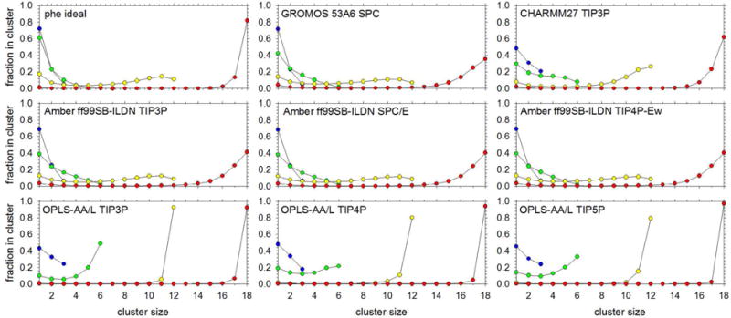
Plots show the fraction of solute molecules that are members of clusters of various sizes at each of the following solute concentrations: 50 (blue), 100 (green), 200 (yellow) and 300 mg/ml (red). The maximum cluster size at each concentration is limited by the total number of solute molecules in the simulation: the maximum sizes are 3, 6, 12, and 18 molecules for 50, 100, 200 and 300 mg/ml, respectively. The panel marked ‘phe ideal’ (top left) shows the distribution of cluster sizes obtained when solute molecules are randomly placed within the simulation box (see text).

The aggregation seen in the OPLS-AA/L simulations is, at the higher solute concentrations, essentially irreversible; as such, it prevents us from adequately sampling the kinetic and thermodynamic behavior of the solutions. Because of this, the OPLS-AA/L results are omitted from the further analyses described below.

Variation of inter-solute interactions with increasing solute concentration

For the remaining force field combinations, an important question that can be addressed with the simulation data is the extent to which different kinds of energetically favorable interactions are affected by increasing solute concentrations. We begin with an analysis of the salt bridge interactions between the amino and carboxyl groups of the amino acids. Representative plots of the radial distribution functions (RDFs) obtained from the simulations of glycine solutions are shown for the Amber ff99SB-ILDN, CHARMM27 and GROMOS 53A6 force fields in Figure 5; corresponding plots for all force field combinations and for the three other types of amino acids are provided in Figures S10 and Figures S11. It is immediately obvious that there are huge differences between the strengths of the salt bridge interactions with the three force fields: with GROMOS 53A6 the salt bridge interactions are of only marginal stability, with Amber ff99SB-ILDN they are stronger and with CHARMM27 they are extremely strong (in passing it should be noted that OPLS-AA/L exhibits a similarly strong salt bridge interaction). We note that there appears to be a strong relationship between the maximum value of these RDFs and the separation distances at which they are maximal (Figure S12): this strongly suggests that a principal cause of the large differences between the force fields is the Lennard-Jones parameters that determine how closely atoms can approach one another. Although these large differences between salt bridge strengths are somewhat surprising it is perhaps more interesting to note that they appear to lead to qualitative differences in the way the strengths of these interactions respond to increasing solute concentration (see insets to Figure 5): with GROMOS 53A6 there is a modest but clear strengthening of the interaction from 50 to 300 mg/ml, with Amber ff99SB-ILDN there is little change, and with CHARMM27 there is a very significant weakening of the interaction. We do not see any obvious change in the separation distance at which the RDF is maximal with increasing solute concentration (Figure 5).

Figure 5. Radial distribution functions for salt bridge interactions in simulations of glycine solutions.

Plots show the radial distribution function for the intermolecular interactions of the carboxylate oxygens and the amino nitrogen; for each molecule pair only the closest distance between either carboxyl oxygen and the amino nitrogen is used in the calculation of the RDF. Results are shown for each of the following solute concentrations: 50 (blue), 100 (green), 200 (yellow) and 300 mg/ml (red). Note the differences in the vertical scale between each of the three sets of results shown. Insets show close-up views of the first peak in the RDF.

These differences in the concentration dependences can be compared more clearly by converting the first peaks of the RDFs into free energy form and plotting these values relative to the value calculated at 50 mg/ml. Figure 6 shows how these effective relative free energies of interaction vary with increasing solute concentration for each of the amino acids. Although there are some differences between them, it is clear that in general the GROMOS 53A6 force field predicts that with increasing solute concentration the salt bridge interaction will be stabilized, by up to 0.12 kcal/mol in the case of valine, although it is very slightly destabilized (by 0.01 kcal/mol) in the case of asparagine. In contrast, the CHARMM27 force field predicts that the salt bridge interaction will be destabilized by anywhere from 0.18 kcal/mol in the case of valine to 0.59 kcal/mol in the case of glycine. For the Amber ff99SB-ILDN force field there is considerable variability between amino acids: for glycine and valine the strength of the salt bridge interaction is essentially independent of the solute concentration, whereas for asparagine and phenylalanine it becomes somewhat weaker as the solute concentration increases. Importantly, there is an essentially linear relationship between the change in the strength of the salt bridge interaction as a function of solute concentration and the intrinsic strength of the interaction as reflected in its value at 50 mg/ml (Figure 7). Notably, this relationship also extends to capturing the differences between the four amino acids simulated with the Amber ff99SB-ILDN force field: within the framework of this relationship, the greater concentration dependence of the asparagine and phenylalanine interactions is consistent with their simulated interactions being more favorable at 50 mg/ml than those of glycine and valine (Figure 7).

Figure 6. Relative effective free energies of interactions for salt bridges in simulations of solutions of all four amino acid types.

Plots show the effective ΔG for the salt bridge interactions relative to the values obtained from simulations performed at 50 mg/ml; clockwise from the top-left: glycine, valine, phenylalanine, asparagine. Results are shown for each of the following force field and water model combinations: Amber ff99SB-ILDN + TIP3P (blue circle), Amber ff99SB-ILDN + TIP4P-Ew (blue triangle), Amber ff99SB-ILDN + SPC/E (blue square), CHARMM27 + TIP3P (green), GROMOS 53A6 + SPC (red).

Figure 7. Relationship between the concentration dependence of the salt bridge ΔG and the intrinsic strength of the interaction at 50 mg/ml.

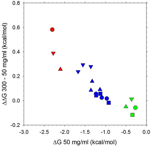
Plots show the difference, ΔΔG, between the ΔG of the salt bridge interaction at 300 mg/ml and the ΔG at 50 mg/ml versus the ΔG at 50 mg/ml. Results are shown for Amber ff99SB-ILDN (blue), CHARMM27 (green), GROMOS 53A6 (red), and for glycine (circle), valine (square), phenylalanine (upward triangle), asparagine (downward triangle). Note that there is no data point for CHARMM27 with valine (green square) as this simulation was considered to have irreversibly aggregated; note also that for Amber ff99SB-ILDN, three results are shown for each amino acid, each corresponding to a different water model.

To examine whether differences might also be observed between the various force fields' descriptions of sidechain interactions we carried out similar analyses on the sidechain interactions of valine, phenylalanine and asparagine. Figure 8 shows RDFs for the interactions of valine sidechains with the Amber ff99SB-ILDN, CHARMM27 and GROMOS 53A6 force fields; corresponding plots for all force field combinations are provided in Figure S13. For these interactions, which we view as being representative of typical aliphatic interactions, there is a much greater degree of correspondence between the various simulation force fields, both in terms of the intrinsic strengths of the interactions and in terms of their dependences on solute concentration. One obvious outlier in Figure 8 is the 300 mg/ml simulation with CHARMM27 which, as noted above, effectively ‘crashed out’: the resulting RDF for this concentration is clearly crazy; for lower concentrations, however, the behavior closely mirrors that seen with Amber ff99SB-ILDN and GROMOS 53A6. In all of the other simulations, a clear peak in the RDF is observed at ∼4 Å with a maximal value ranging from 1.78 (GROMOS 53A6) to 2.53 (Amber ff99SB-ILDN + TIP3P) which increases modestly as the solute concentration increases. As before, these changes can be converted into an effective free energy form (Figure S14): depending on the force field combination used, increasing the solute concentration from 50 to 300 mg/ml causes a stabilization of the effective free energy of interaction between the sidechains ranging from 0.06 (Amber ff99SB-ILDN + TIP3P) to 0.18 (GROMOS 53A6) kcal/mol.

Figure 8. Radial distribution functions for sidechain interactions in selected simulations of valine solutions.

Plots show the radial distribution function for the intermolecular interactions of sidechain atoms; for each molecule pair only the closest distance between any pair of sidechain heavy atoms is used in the calculation of the RDF. Results are shown for each of the following solute concentrations: 50 (blue), 100 (green), 200 (yellow) and 300 mg/ml (red). Insets show close-up views of the first peak in the RDF.

To examine whether differences might also be observed between the various force fields' descriptions of sidechain interactions we carried out similar analyses on the sidechain interactions of valine, phenylalanine and asparagine. Figure 8 shows RDFs for the interactions of valine sidechains with the Amber ff99SB-ILDN, CHARMM27 and GROMOS 53A6 force fields; corresponding plots for all force field combinations are provided in Figure S13. For these interactions, which we view as being representative of typical aliphatic interactions, there is a much greater degree of correspondence between the various simulation force fields, both in terms of the intrinsic strengths of the interactions and in terms of their dependences on solute concentration. One obvious outlier in Figure 8 is the 300 mg/ml simulation with CHARMM27 which, as noted above, effectively ‘crashed out’: the resulting RDF for this concentration is clearly crazy; for lower concentrations, however, the behavior closely mirrors that seen with Amber ff99SB-ILDN and GROMOS 53A6. In all of the other simulations, a clear peak in the RDF is observed at ∼4 Å with a maximal value ranging from 1.78 (GROMOS 53A6) to 2.53 (Amber ff99SB-ILDN + TIP3P) which increases modestly as the solute concentration increases. As before, these changes can be converted into an effective free energy form (Figure S14): depending on the force field combination used, increasing the solute concentration from 50 to 300 mg/ml causes a stabilization of the effective free energy of interaction between the sidechains ranging from 0.06 (Amber ff99SB-ILDN + TIP3P) to 0.18 (GROMOS 53A6) kcal/mol.

While the behavior of the aliphatic interactions appears to be consistently predicted by the various simulation force fields, differences are again observed when we examine aromatic interactions in the phenylalanine simulations (Figure 9;Figure S15;see Figure S16 for ΔΔG). Amber ff99SB-ILDN, GROMOS 53A6 and CHARMM27 all produce highly comparable strengths of interactions, but they differ qualitatively in their predictions of the concentration dependences: with Amber ff99SB-ILDN, the aromatic interaction is predicted to become progressively weaker as the solute concentration increases, but with GROMOS 53A6 and CHARMM27 the interaction is predicted to become stronger. In contrast to what was seen with the salt bridge interaction, therefore, the qualitatively different concentration dependences of the force fields do not appear to have any clear connection with the intrinsic strengths of the interaction: the heights of the RDFs range only from 4.82 (GROMOS 53A6) to 5.12 (Amber ff99SB-ILDN + SPC).

Figure 9. Radial distribution functions for sidechain interactions in selected simulations of phenylalanine solutions.

Plots show the radial distribution function for the intermolecular interactions of sidechain atoms; for each molecule pair only the closest distance between any pair of sidechain heavy atoms is used in the calculation of the RDF. Results are shown for each of the following solute concentrations: 50 (blue), 100 (green), 200 (yellow) and 300 mg/ml (red). Insets show close-up views of the first peak in the RDF.

In an attempt to uncover an explanation for the qualitative differences in the concentration dependences we examined the interaction geometries of the phenylalanine sidechains. To this end, we analyzed all cases where phenylalanine sidechains were in contact (heavy atom distance < 4.5 Å) and constructed histograms of the angle between the vectors normal to the planes of the aromatic rings. The resulting histograms for three of the force fields are plotted in Figure 10. With Amber ff99SB-ILDN, at 50 mg/ml (blue symbols) the distribution peaks at ∼55° and plateaus at ∼90°; a comparatively high frequency at 90° is expected on purely geometric grounds as it corresponds to the most common value sampled when rings are randomly oriented relative to one another (the random distribution follows a sinusoidal dependence upon the angle).⁶⁹ In contrast, with GROMOS 53A6, the distribution is high through the range ∼65° to 90° and only a weak shoulder is observed at ∼55°. Despite these differences, the force fields are in striking agreement on the concentration dependences of these two populations: both force fields predict that configurations with angles of ∼55° are destabilized while configurations with angles of ∼90° are stabilized by increasing solute concentration (see insets on Figure 10). The same qualitative result is obtained with CHARMM27 although the overall shape of the distribution in this case is intermediate between those of Amber ff99SB-ILDN and GROMOS 53A6. The qualitative differences observed in the aromatic RDFs between the various force fields (Figure 9) appear, therefore, to be a consequence of differences in their predicted geometries of interaction of the aromatic rings.

Figure 10. Probability distributions of intermolecular aromatic ring geometries sampled during selected simulations of phenylalanine solutions.

Plots show the probability distribution of the angle between the vectors normal to the aromatic rings of contacting phenylalanine molecules; the distribution is calculated for all pairs of phenylalanine molecules with a pair of ring heavy atoms within 4.5 Å of each other. Results are shown for each of the following solute concentrations: 50 (blue), 100 (green), 200 (yellow) and 300 mg/ml (red). Insets at top-left show close-up views of the distribution around 52.5°; insets at bottom-right show close-up views of the distribution around 82.5°.

Finally, Figure 11 shows RDFs for the sidechain interactions in the asparagine simulations. In comparison with the other interactions that we have examined, the shapes of the RDFs for interactions of the asparagine sidechains are considerably more complicated, containing a number of peaks reflecting the greater chemical heterogeneity of the sidechain. Despite this, the Amber force field quite clearly predicts that the interactions of become much weaker with increasing solute concentration while those with the GROMOS force field become somewhat weaker. For CHARMM27, the behavior seems to be similar to that predicted by GROMOS 53A6, although in this case the potentially confounding presence of the salt bridge interactions is more pronounced (note the additional peaks in the range 6–8 Å).

Figure 11. Radial distribution functions for sidechain interactions in selected simulations of asparagine solutions.

Plots show the radial distribution function for the intermolecular interactions of sidechain atoms; for each molecule pair only the closest distance between any pair of sidechain heavy atoms is used in the calculation of the RDF. Results are shown for each of the following solute concentrations: 50 (blue), 100 (green), 200 (yellow) and 300 mg/ml (red). Insets show close-up views of the first peak in the RDF.

Discussion

The overall goal of this study has been to use all-atom, explicit-solvent, MD simulations to determine the effects that increasing solute concentrations up to the levels encountered inside biological cells would have upon on the thermodynamics of typical electrostatic and hydrophobic interactions. Prior to doing this, however, we first attempted to verify that the simulation force fields produced solution behavior that was at least to some degree consistent with experiment. Overall, most of the simulation force fields produce behavior that is in reasonably good agreement with experiment: all perform very well with respect to reproducing solution densities, and while they have trouble capturing the breadth of the range of viscosity increments and the narrowness of the range of dielectric increments, the trends are, in general, reproduced quite well.

It is to be noted, of course, that all of the amino acids studied here are, in reality, insoluble at the highest concentrations that we have simulated. While this is certainly true at the macroscopic level, it is not clear, however, whether it should be true at the microscopic level of the current simulations: at 300 mg/ml, for example, our simulations of phenylalanine contain only 18 solute molecules and it seems unlikely that even a conglomerate of all 18 molecules could be considered large enough to constitute a true solid phase. Because of this, the fact that most of the amino acids remain soluble when simulated with most of the force field combinations should not be considered necessarily incorrect; by the same token, however, nor should the extensive aggregation seen with the OPLS-AA/L force field be considered definitively incorrect. One way to lay this issue to rest in the future would be to attempt explicit calculations of the solubility with the same force field combinations used here. How best to calculate solubility from first principles is an active area of research⁷⁰ but recent work⁷¹ has shown that MD simulation methodologies can be used to perform such calculations with reasonable accuracy for relatively simple organic solutes; performing such calculations for amino acids with sufficient accuracy is, however, likely to be more difficult given their zwitterionic nature and the very large changes in electrostatic energy contributions that will inevitably be involved.

One closely related area where there has already been considerable use of explicit-solvent MD simulations is in modeling the crystallization of glycine from aqueous solution.^72-78 Glycine is an attractive model system for studying biomolecular crystallization processes, and since modeling crystallization necessitates the use of high solute concentrations, a number of simulation studies have been reported that make comparison with experimental solution densities; none of these studies, however, has addressed the viscosity and dielectric increments or the relative strengths of inter-molecular interactions that have been explored here. Of special relevance to this work, however, is the study by Cheong and Boon⁷⁸ who simulated a range of glycine concentrations using a large number of different force field combinations including three – CHARMM27, OPLS-AA/L and GROMOS 53A6 – that have been examined here. Although their simulations were much shorter than those presented here (2 ns versus the 1 μs used here), their results for the solution densities predicted by these force fields are in agreement with ours. Their work emphasized the importance of electrostatic interactions of glycine's charged termini in determining overall behavior, and they explicitly showed that changing only the partial charges could lead to quite different crystallization behavior.⁷⁸ They also showed that force fields that give the best lattice energies and crystal parameters do not necessarily give the best description of behavior in the aqueous solution phase; solving this issue is likely to require polarizable force fields.⁷¹

In terms of comparing our density, viscosity and dielectric increments with experiment, it would obviously be nice to sidestep solubility questions entirely by performing simulations at solute concentrations where they are all experimentally soluble. But a simulation of phenylalanine at 25 mg/ml using the box size used here, for example, would involve the inclusion of only 1.5 solute molecules; in order to perform such measurements in a meaningful way, therefore, would require considerably larger simulation boxes to be used. The computational expense associated with simulating larger systems would be exacerbated by the fact that longer simulations would likely be required in order to obtain converged results (due to the more infrequent sampling of association events) and to measure accurately what will undoubtedly be a weaker effect owing to the lower solute concentration. At the moment, therefore, the expense involved in such calculations would prevent us from drawing clear conclusions for the variety of systems and force field combinations studied here. Perhaps more importantly, however, the very clear and smooth concentration dependences that we obtain here over the range of concentrations from 50 to 300 mg/ml (e.g. Figures 1 to 3) suggest that there is not much to be gained from repeating the simulations at lower concentrations.

While the density increments calculated with all force field combinations are in good agreement with experiment, the apparent discrepancies with regard to other solution properties are worth examining in a little more detail. With regard to the viscosity increments, it is notable that all of the force field combinations do well at reproducing the relative values for glycine, valine and phenylalanine, all of which were measured by the same experimental group. Where there is disagreement with experiment is in the relative value for asparagine. It is therefore tempting to consider that the experimental value for asparagine might be in doubt; specifically, it might be too high. Arguing against this idea, however, is the fact that Palani and Geetha⁵⁹ have also reported data for asparagine, and when we convert their data so that they are on the same scale as those reported by Thirumaran et al.,⁵⁸ (0.606 mPa.s/M) we find that their measured viscosity increment (0.635 mPa.s/M) is somewhat higher (see Methods). Given that the simulation force fields predict with near unanimity that the viscosity increment of asparagine should be less than not only that of phenylalanine but also that of valine, it appears that clearing up this discrepancy with experiment might be worth investigation. In particular, if experiments performed under identical laboratory conditions indicate that the viscosity increment of asparagine is indeed higher than that of both valine and phenylalanine this would indicate that there is something fundamentally wrong with the force field descriptions of these amino acids. On the other hand, if further experiments indicate that asparagine's viscosity increment is lower than that of phenylalanine and comparable to, or lower than that of valine, it would provide an important example of the use of molecular simulations to guide experimental studies.

Similar questions arise with the dielectric increments. It is worth noting that in the early days of experimental measurements – which were some eighty years ago (reviewed in ref. 66) – systematic differences were noted between the values reported by different groups. It is therefore worth noting that the data that we have most confidence in – those reported by Suzuki et al.⁶² for phenylalanine and valine – are qualitatively reproduced by the Amber ff99SB-ILDN, GROMOS 53A6 and CHARMM27 force fields and by OPLS-AA/L when used with the TIP3P water model. Similarly, it is worth noting that the data reported in the 1930's by Devoto^60,61 for valine, glycine and asparagine are also qualitatively reproduced by the Amber ff99SB-ILDN force field. Despite these points of qualitative agreement with experiment there are significant quantitative discrepancies: the dielectric increments of phenylalanine and valine computed with Amber ff99SB-ILDN, for example, are all less than 10 M⁻¹ whereas the corresponding experimental values are ∼20 M⁻¹. The results obtained with CHARMM27 are also uniformly lower than experiment, which stands in interesting contrast to the results of Boresch et al.⁶⁷ who used the earlier CHARMM Param 19⁷⁹ polar hydrogen force field together with CHARMM-modified TIP3P water model to model the dielectric increment of alanine solutions and obtained a value that was 32.3 M⁻¹, somewhat higher than the reported experimental value of 22.7 M⁻¹.

In addition to these differences with experiment, there are clear differences between the various force fields in terms of their predictions for the relative dielectric increments of glycine and asparagine: the Amber ff99SB-ILDN force field predicts that asparagine should have a higher dielectric increment than glycine – which incidentally is in agreement with the data reported by Devoto^60,61 – while the CHARMM27, GROMOS 53A6 and OPLS-AA/L force fields (with the exception of the simulation using TIP5P water) all predict the opposite result. It seems likely, therefore, that new experimental measurements of these dielectric increments would go a long way toward resolving this clear point of disagreement. Finally, it is worth noting that the narrowness of the measured experimental values – which is difficult for the simulations to capture – appears to be real: experimental data for other zwitterionic α-amino acids, for example, are all within the same range of 20-30.⁶⁶

The comparisons that we have made with experimental data on the solution properties of amino acid solutions can be considered complementary to other force field comparison studies that have recently been reported in the literature. In particular, a number of recent MD studies have compared the conformational behavior of peptides and proteins predicted by non-polarizable protein force fields with a variety of experimental NMR observables.^80-85 In general, these studies have indicated that all of the extant force fields perform reasonably well and that, while some clearly appear to perform better than others, there are no truly drastic discrepancies between them. Here, however, we have shown that there are enormous differences between the different force fields' descriptions of the thermodynamics of terminal salt bridge interactions: specifically, we find that CHARMM27 (and OPLS-AA/L) predict very strong interactions, with Amber ff99SB-ILDN and GROMOS 53A6 predicting progressively weaker interactions. At least qualitatively, this ordering appears consistent with the results of previous simulation studies scattered in the literature that have measured the potential of mean force (PMF) for salt bridge interactions between lysine and glutamate sidechains. Yuzlenko and Lazaridis measured an interaction free energy at the PMF minimum of −1.8 kcal/mol with CHARMM27 and TIP3P;⁸⁶ Geney et al., measured an interaction of −1.2 kcal/mol with Amber ff99 and TIP3P in a conformationally constrained peptide,⁸⁷ and Nguyen et al., measured an interaction of −1.5 kcal/mol with Amber ff99SB and TIP3P in the same model system.⁸⁸ Wassenaar et al.⁸⁹ measured an interaction of −0.76 kcal/mol with GROMOS53A6 and SPC/E, while de Jong et al.⁹⁰ recently reported a free energy of −0.05 kcal/mol for lysine and glutamate analogs using GROMOS53A6 and SPC. The latter authors also reported an interaction free energy of −0.80 kcal/mol for OPLSAA/L, which appears somewhat less strong than what we estimate for the salt bridge interaction of glycine amino acids (data not shown).

It could certainly be argued that differences in the interactions of amino acid termini are of little consequence given that the principal use of biomolecular force fields is to simulate proteins and not individual amino acids; it is also worthwhile noting that parameterization of terminal groups appears to typically receive less attention than that of sidechain groups. But, for the following reasons, we think that it is quite likely that significant differences between the force fields will also be seen in the interactions of the charged amino acid sidechains. This is because the atom types used for atoms of the terminal NH₃⁺ and COO⁻ groups are identical to those used for the lysine and glutamate sidechains in each of the force fields (i.e. they share the same Lennard-Jones parameters). In addition, the terminal and charged sidechain groups possess identical sets of partial charges in the GROMOS 53A6 and OPLS-AA/L force fields, identical NH₃⁺ and similar COO⁻ partial charges in the CHARMM27 force field and similar COO⁻ and NH₃⁺ partial charges in the Amber ff99SB-ILDN force field. For these reasons, and because charged sidechains are often the first point of contact between associating proteins it is probable, therefore, that the differences observed here would also be reflected in differences between the force fields' descriptions of protein-protein interactions. Because of this, one goal that might be worth pursuing in the near future is to compare the predictions of the force fields with experimental data on the thermodynamics of mutating charged residues in protein-protein interfaces, such as in the classic electrostatically-driven barnase-barstar complex.⁹¹ These data have previously been the subject of calculations⁹² using the Poisson-Boltzmann (PB) continuum electrostatic model, and have provided valuable information for identifying which calculation protocols are likely to perform the best in general applications.⁹³ A more recent study⁹⁴ has shown that the desolvation thermodynamics of charged residues in the barnase-barstar complex can be computed using explicit-solvent MD simulations, with the results being in surprisingly good agreement with those calculated using the PB method. This good agreement between the two approaches has also very recently been shown⁹⁵ to extend to the very high temperatures that are applicable to hyperthermophiles, for which salt bridge interactions appear crucially important.^96,97 Given, therefore, that the barnase-barstar system has previously proven useful for identifying areas for improvement in implicit-solvent PB electrostatics calculations, it seems reasonable to suggest that it might fulfill a similar role in identifying which – if any – of the explicit-solvent force fields studied here are likely to give a good description of salt bridge interactions in proteins in aqueous solution.

It is worth stressing that we think that the most likely cause of the large differences in salt bridge interactions between the force fields are not the partial charge sets but are instead the Lennard-Jones parameters assigned to the atoms. We state this because there is a very clear correlation between the maximal value of the salt bridge RDF and the separation distance at which the RDF is maximal (Figure S10). This inverse correlation implies that as the charged atoms approach each other more closely their electrostatic interaction becomes more favorable which in turn suggests that, if necessary, reparameterization of salt bridge interactions in the force fields should be achievable by scaling the effective atomic radii of the Lennard-Jones interactions. Of course, this would have to be done in such a way that it does not alter interactions with water as many of the simulation force fields have been parameterized to reproduce the hydration free energies of the charged amino acids (we note that this is also true of a new variant of the GROMOS force field⁹⁸ that was reported recently). It is to be remembered that Cheong & Boon⁷⁷ have shown that the crystallization behavior of glycine in simulations can be very sensitive to the choice of partial charges, which suggests that these might also be reparameterized; doing so, however, would also upset the description of solute-water interactions in a way that would be much less easy to control.

While settling on a description of salt bridge interactions is likely to be important for correctly describing the role of charged residues in modulating the thermodynamics of protein stability and protein-protein interactions, the results presented here suggest another reason why this would be important to resolve. This is the result shown in Figure 7 which indicates that there is a strong relationship between the intrinsic strength of the salt bridge interaction and its qualitative dependence on the solute concentration. It is not completely clear to us why such a relationship should exist, but it is nevertheless likely to be important to remember for (future) comparisons between thermodynamic behavior in dilute solution and in the highly crowded environments encountered in biological cells: it is quite possible, for example, that depending on the intrinsic strength of the interaction, qualitatively different conclusions could be drawn as to whether salt bridge interactions are likely to be strengthened or weakened in intracellular conditions.

Encouragingly, while there are very large differences between the force fields' descriptions of salt bridge interactions there are no major differences between their descriptions of aliphatic interactions: all of them predict that the effective free energy of interaction of valine sidechains should be in the range −0.34 (GROMOS 53A6) to −0.55 (Amber ff99SB-ILDN + TIP3P) kcal/mol. Perhaps more importantly, all of the force fields also predict that these interactions will become more favorable as the solute concentration increases (and/or as the level of hydration decreases). Given the wide range of force field combinations studied here, the idea that sidechain interactions of hydrophobic residues such as valine become stronger in crowded conditions is likely to be a consistent prediction of all pairwise protein force fields. If correct, this predicted result could have significant implications for understanding protein stability in vivo. In passing, it is also worth comparing our results with previous MD simulation studies of the concentration dependence of interactions between the simple hydrocarbon methane in water:^99-101 while the latter have suggested that the hydrophobic interaction is essentially independent of concentration at low concentrations, they have also suggested that a cooperative transition occurs at higher concentrations so that the addition of an extra molecule to an existing cluster becomes increasingly favorable.^99,101 This transition does not appear in the present study – the plots of ΔΔG versus concentration appear to be essentially linear (Figure S12) – but nor is it necessarily expected to appear since the hydrocarbon sidechains in our simulations are inseparable from their peptide backbones: intermolecular associations in the present systems, therefore, involve not only the favorable dehydration of the nonpolar sidechains but also the unfavorable dehydration of the polar backbone atoms.

Interestingly, the close correspondence between the force fields' descriptions of aliphatic interactions does not extend to their descriptions of aromatic interactions: while the Amber ff99SB-ILDN, CHARMM27 and GROMOS 53A6 force fields all predict effective free energies of interaction in the very narrow range −0.94 to −0.97 kcal/mol, the former predicts that increasing solute concentration leads to a destabilization of the interaction while the latter two predict a stabilization. We have attempted to determine the origins of these differences by exploring the geometries the of ring-ring interactions in a way pioneered some years ago by Burley and Petsko.¹⁰² Although there are more sophisticated ways of comparing the interaction geometries of phenylalanine rings^{69,90,103-105} the relatively simple approach used here already indicates that there are some surprising differences between the force fields (Figure 10) and that different interaction geometries have qualitatively different responses to increasing solute concentrations. Interestingly, comparison of the partial charges assigned to the phenylalanine rings does not show any obvious differences that would be expected to cause these differences between the force fields; it is possible, therefore, that the observed differences might reflect the presence and influence of other types of interactions, especially the salt bridge interactions. Unfortunately, it is difficult to determine which of the distributions is likely to be most realistic: comparisons with the corresponding distributions in protein structures, for example, is unlikely to be informative as the latter are subject to much greater conformational constraints than are the free amino acids simulated here.

In summary, we have found a number of similarities and differences between the force fields examined here both in terms of the intrinsic strengths of amino acid interactions and in terms of their dependences on solute concentration. For salt bridge interactions there are clearly huge differences between the force fields' descriptions of the thermodynamics and these differences lead to surprising qualitative differences in their concentration dependences. For the aliphatic interactions of valine sidechains, the force fields are all in much closer agreement and, in particular, all agree that the interactions should become more favorable at higher solute concentrations. Perhaps most intriguingly, for the aromatic interactions of phenylalanine sidechains, the force fields agree on the effective free energy of interaction but differ considerably on the interaction geometries and, apparently as a consequence, on the concentration dependences of the interaction thermodynamics. Taken together, the significant differences between the concentration dependences predicted by the different simulation force fields suggest that, until such differences are resolved, caution may need to be exercised in interpreting the results of MD simulations performed on crowded macromolecular systems.

We note in closing that while we have focused here on force fields that are all widely used for simulations of proteins and other macromolecules, a very attractive alternative, at least with respect to simulations of small solutes, is the Kirkwood-Buff Derived Force Field (KBFF) being developed by the Smith group.^106,107 The philosophy behind the KBFF places greater emphasis on correctly reproducing the experimentally derived thermodynamics of solute-solute and solute-solvent interactions; importantly, KBFF simulations of glycine solutions have already been shown to produce quite good agreement with experimental osmotic virial coefficients.¹⁰⁸ We also note in closing that there are other simulation observables that could be compared between the force fields studied here. In particular, the description of translational and rotational diffusion of both the solutes and the solvent are subjects of interest given that high solute concentrations are associated with substantial alterations to diffusion in vivo.⁵ A preliminary examination of these properties in the present systems suggests, however, that their behavior is sufficiently complicated to warrant a more detailed study; this will be the subject of future work.

References

- 1.Fulton AB. How Crowded Is the Cytoplasm? Cell. 1982;30:345–347. doi: 10.1016/0092-8674(82)90231-8. [DOI] [PubMed] [Google Scholar]
- 2.Ellis RJ, Minton AP. Cell biology - Join the crowd. Nature. 2003;425:27–28. doi: 10.1038/425027a. [DOI] [PubMed] [Google Scholar]
- 3.Zimmerman SB, Trach SO. Estimation of Macromolecule Concentrations and Excluded Volume Effects for the Cytoplasm of Escherichia-Coli. J Mol Biol. 1991;222:599–620. doi: 10.1016/0022-2836(91)90499-v. [DOI] [PubMed] [Google Scholar]
- 4.Elowitz MB, Surette MG, Wolf PE, Stock JB, Leibler S. Protein mobility in the cytoplasm of Escherichia coli. J Bacteriol. 1999;181:197–203. doi: 10.1128/jb.181.1.197-203.1999. [DOI] [PMC free article] [PubMed] [Google Scholar]
- 5.Dix JA, Verkman AS. Crowding effects on diffusion in solutions and cells. Annu Rev Biophys. 2008;37:247–263. doi: 10.1146/annurev.biophys.37.032807.125824. [DOI] [PubMed] [Google Scholar]
- 6.Ghaemmaghami S, Oas TG. Quantitative protein stability measurement in vivo. Nature Struct Biol. 2001;8:879–882. doi: 10.1038/nsb1001-879. [DOI] [PubMed] [Google Scholar]
- 7.Ignatova Z, Krishnan B, Bombardier JP, Marcelino AMC, Hong J, Gierasch LM. From the test tube to the cell: exploring the folding and aggregation of a beta-clam protein. Biopolymers. 2007;88:157–163. doi: 10.1002/bip.20665. [DOI] [PMC free article] [PubMed] [Google Scholar]
- 8.Ebbinghaus S, Dhar A, McDonald JD, Gruebele M. Protein folding stability and dynamics imaged in a living cell. Nature Methods. 2010;7:319–323. doi: 10.1038/nmeth.1435. [DOI] [PubMed] [Google Scholar]
- 9.Dhar A, Girdhar K, Singh D, Gelman H, Ebbinghaus S, Gruebele M. Protein stability and folding kinetics in the nucleus and endoplasmic reticulum of eukaryotic cells. Biophys J. 2011;101:421–430. doi: 10.1016/j.bpj.2011.05.071. [DOI] [PMC free article] [PubMed] [Google Scholar]
- 10.Phillip Y, Kiss V, Schreiber G. Protein-binding dynamics imaged in a living cell. Proc Natl Acad Sci USA. 2012;109:1461–1466. doi: 10.1073/pnas.1112171109. [DOI] [PMC free article] [PubMed] [Google Scholar]
- 11.Zhou HX, Rivas G, Minton AP. Macromolecular crowding and confinement: biochemical, biophysical, and potential physiological consequences. Annu Rev Biophys. 2008;37:375–397. doi: 10.1146/annurev.biophys.37.032807.125817. [DOI] [PMC free article] [PubMed] [Google Scholar]
- 12.Elcock AH. Models of macromolecular crowding effects and the need for quantitative comparisons with experiment. Curr Opin Struct Biol. 2010;20:196–206. doi: 10.1016/j.sbi.2010.01.008. [DOI] [PMC free article] [PubMed] [Google Scholar]
- 13.Yap EH, Head-Gordon T. Calculating the bimolecular rate of protein-protein association with interacting crowders. J Chem Theory Comput. 2013;9:2481–2489. doi: 10.1021/ct400048q. [DOI] [PubMed] [Google Scholar]
- 14.Frembgen-Kesner T, Elcock AH. Computer simulations of the bacterial cytoplasm. Biophys Rev. 2013;5:109–119. doi: 10.1007/s12551-013-0110-6. [DOI] [PMC free article] [PubMed] [Google Scholar]
- 15.Bicout DJ, Field MJ. Stochastic dynamics simulations of macromolecular diffusion in a model of the cytoplasm of Escherichia coli. J Phys Chem. 1996;100:2489–2497. [Google Scholar]
- 16.Ridgway D, Broderick G, Lopez-Campistrous A, Ru'aini M, Winter P, Hamilton M, Boulanger P, Kovalenko A, Ellison MJ. Coarse-grained molecular simulation of diffusion and reaction kinetics in a crowded virtual cytoplasm. Biophys J. 2008;94:3748–3759. doi: 10.1529/biophysj.107.116053. [DOI] [PMC free article] [PubMed] [Google Scholar]
- 17.McGuffee SR, Elcock AH. Diffusion, crowding & protein stability in a dynamic molecular model of the bacterial cytoplasm. PLoS Comput Biol. 2010;6:e1000694. doi: 10.1371/journal.pcbi.1000694. [DOI] [PMC free article] [PubMed] [Google Scholar]
- 18.Ando T, Skolnick J. Crowding and hydrodynamic interactions likely dominate in vivo macromolecular motion. Proc Natl Acad Sci USA. 2010;107:18457–18462. doi: 10.1073/pnas.1011354107. [DOI] [PMC free article] [PubMed] [Google Scholar]
- 19.Frembgen-Kesner T, Elcock AH. Striking effects of hydrodynamic interactions on the simulated diffusion and folding of proteins. J Chem Theory Comput. 2009;5:242–256. doi: 10.1021/ct800499p. [DOI] [PubMed] [Google Scholar]
- 20.Mereghetti P, Wade RC. Atomic detail Brownian dynamics simulations of concentrated protein solutions with a mean field treatment of hydrodynamic interactions. J Phys Chem B. 2012;116:8523–8533. doi: 10.1021/jp212532h. [DOI] [PubMed] [Google Scholar]
- 21.Cossins B, Jacobson MP, Guallar V. A new view of the bacterial cytosol environment. PLoS Comput Biol. 2011;7:e1002066. doi: 10.1371/journal.pcbi.1002066. [DOI] [PMC free article] [PubMed] [Google Scholar]
- 22.Harada R, Sugita Y, Feig M. Protein crowding affects hydration structure and dynamics. J Am Chem Soc. 2012;134:4842–4849. doi: 10.1021/ja211115q. [DOI] [PMC free article] [PubMed] [Google Scholar]
- 23.Feig M, Sugita Y. Variable interactions between protein crowders and biomolecular solutes are important in understanding cellular crowding. J Phys Chem B. 2012;116:599–605. doi: 10.1021/jp209302e. [DOI] [PMC free article] [PubMed] [Google Scholar]
- 24.Miklos AC, Sarkar M, Wang Y, Pielak GJ. Protein crowding tunes protein stability. J Am Chem Soc. 2011;133:7116–7120. doi: 10.1021/ja200067p. [DOI] [PubMed] [Google Scholar]
- 25.van der Spoel D, Lindahl E, Hess B, Groenhof G, Mark AE, Berendsen HJC. GROMACS: fast, flexible, free. J Comput Chem. 2005;26:1701–1718. doi: 10.1002/jcc.20291. [DOI] [PubMed] [Google Scholar]
- 26.Hess B, Kutzner C, van der Spoel D, Lindahl E. GROMACS 4: algorithms for highly efficient, load-balanced, and scalable molecular simulation. J Chem Theory Comput. 2008;4:435–447. doi: 10.1021/ct700301q. [DOI] [PubMed] [Google Scholar]
- 27.Nosé S. A unified formulation of the constant temperature molecular-dynamics methods. J Chem Phys. 1984;81:511–519. [Google Scholar]
- 28.Hoover WG. Canonical dynamics – equilibrium phase-space distributions. Phys Rev A. 1985;31:1695–1697. doi: 10.1103/physreva.31.1695. [DOI] [PubMed] [Google Scholar]
- 29.Parrinello M, Rahman A. Polymorphic transitions in single crystals – a new molecular-dynamics method. J Appl Phys. 1981;52:7182–7190. [Google Scholar]
- 30.Essmann U, Perera L, Berkowitz ML, Darden T, Lee H, Pedersen LG. A smooth particle mesh Ewald method. J Chem Phys. 1995;103:8577–8593. [Google Scholar]
- 31.Hess B, Bekker H, Berendsen HJC, Fraaije JGEM. LINCS: a linear constraint solver for molecular simulations. J Comput Chem. 1997;12:1463–1472. [Google Scholar]
- 32.Hornak V, Abel R, Okur A, Strockbine B, Roitberg A, Simmerling C. Comparison of multiple amber force fields and development of improved protein backbone parameters. Proteins Struct Funct Bioinf. 2006;65:712–725. doi: 10.1002/prot.21123. [DOI] [PMC free article] [PubMed] [Google Scholar]
- 33.Lindorff-Larsen K, Piana S, Palmo K, Maragakis P, Klepeis JL, Dror RO, Shaw DE. Improved side-chain torsion potentials for the Amber ff99SB protein force field. Proteins-Struct Funct Bioinf. 2010;78:1950–1958. doi: 10.1002/prot.22711. [DOI] [PMC free article] [PubMed] [Google Scholar]
- 34.Jorgensen WL, Chandrasekhar J, Madura JD, Impey RW, Klein ML. Comparison of simple potential functions for simulating liquid water. J Chem Phys. 1983;79:926–935. [Google Scholar]
- 35.Berendsen HJC, Grigera JR, Straatsma TP. The missing term in effective pair potentials. J Phys Chem. 1987;91:6269–6271. [Google Scholar]
- 36.Horn HW, Swope WC, Pitera JW, Madura JD, Dick TJ, Hura GL, Head-Gordon T. Development of an improved four-site water model for biomolecular simulations: TIP4P-Ew. J Chem Phys. 2004;120:9665–9678. doi: 10.1063/1.1683075. [DOI] [PubMed] [Google Scholar]
- 37.Oostenbrink C, Villa A, Mark AE, van Gunsteren WF. A biomolecular force field based on the free enthalpy of hydration and solvation: the GROMOS force-field parameter sets 53A5 and 53A6. J Comput Chem. 2004;25:1656–1676. doi: 10.1002/jcc.20090. [DOI] [PubMed] [Google Scholar]
- 38.Berendsen HJC, Postma JPM, van Gunsteren WF, Hermans J. Interaction models for water in relation to protein hydration. In: Pullman B, editor. Intermolecular Forces. Reidel, Dordrecht; Holland: 1981. pp. 331–342. [Google Scholar]
- 39.MacKerell AD, Jr, Bashford D, Bellott M, Dunbrack RL, Jr, Evanseck JD, Field MJ, Fischer S, Gao J, Guo H, Ha S, Joseph-McCarthy D, Kuchnir L, Kuczera K, Lau FTK, Mattos C, Michnick S, Ngo T, Nguyen DT, Prodhom B, Reiher WE, III, Roux B, Schlenkrich M, Smith JC, Stote R, Straub J, Watanabe M, Wiórkiewicz-Kuczera J, Yin D, Karplus M. All-atom empirical potential for molecular modeling and dynamics studies of proteins. J Phys Chem B. 1998;102:3586–3616. doi: 10.1021/jp973084f. [DOI] [PubMed] [Google Scholar]
- 40.MacKerell AD, Jr, Feig M, Brooks CL., III Extending the treatment of backbone energetics in protein force fields: limitations of gas-phase quantum mechanics in reproducing protein conformational distributions in molecular dynamics simulations. J Comput Chem. 2004;25:1400–1415. doi: 10.1002/jcc.20065. [DOI] [PubMed] [Google Scholar]
- 41.Kaminski GA, Friesner RA, Tirado-Rives J, Jorgensen WL. Evaluation and reparametrization of the OPLS-AA force field for proteins via comparison with accurate quantum chemical calculations on peptides. J Phys Chem B. 2001;105:6474. [Google Scholar]
- 42.Mahoney MW, Jorgensen WL. A five-site model for liquid water and the reproduction of the density anomaly by rigid, nonpolarizable potential functions. J Chem Phys. 2000;112:8910–8922. [Google Scholar]
- 43.Bjelkmar P, Larsson P, Cuendet MA, Hess B, Lindahl E. Implementation of the CHARMM force field in GROMACS: analysis of protein stability effects from correction maps, virtual interaction sites, and water models. J Chem Theory Comput. 2010;6:459–466. doi: 10.1021/ct900549r. [DOI] [PubMed] [Google Scholar]
- 44.Vanquelef E, Simon S, Marquant G, Garcia E, Klimerak G, Delepine JC, Cieplak P, Dupradeau FY. R.E.D. server: a web service for deriving RESP and ESP charges and building force field libraries for new molecules and molecular fragments. Nucleic Acids Res. 2011;39:W511–W517. doi: 10.1093/nar/gkr288. [DOI] [PMC free article] [PubMed] [Google Scholar]
- 45.Cornell WD, Cieplak P, Bayly CI, Gould IR, Merz KM, Ferguson DM, Spellmeyer DC, Fox T, Caldwell JW, Kollman PA. A second generation force field for the simulation of proteins, nucleic acids and organic molecules. J Am Chem Soc. 1995;117:5179–5197. [Google Scholar]
- 46.Haynes WM, editor. CRC Handbook of Chemistry and Physics. 93. Taylor & Francis; 2012. [Google Scholar]
- 47.Palmer BJ. Transverse-current autocorrelation-function calculations of the shear viscosity for molecular liquids. Phys Rev E. 1994;49:359–366. doi: 10.1103/physreve.49.359. [DOI] [PubMed] [Google Scholar]
- 48.Hess B. Determining the shear viscosity of model liquids from molecular dynamics simulations. J Chem Phys. 2002;116:209–217. [Google Scholar]
- 49.Harris KR, Woolf LA. Temperature and volume dependence of the viscosity of water and heavy water at low temperatures. J Chem Eng Data. 2004;49:1064–1069. [Google Scholar]
- 50.Neumann M. Dipole Moment Fluctuation Formulas in Computer Simulations of Polar Systems. Mol Phys. 1983;50:841–858. [Google Scholar]
- 51.van der Spoel D, van Maaren PJ, Berendsen HJC., III A Systematic Study of Water Models for Molecular Simulation: Derivation of Water Models Optimized for use with a Reaction Field. J Chem Phys. 1998;108:10220–l0230. [Google Scholar]
- 52.Yang L, Weerasinghe S, Smith PE, Pettitt BM. Dielectric response of triplex DNA in ionic solution. Biophys J. 1995;69:1519–1527. doi: 10.1016/S0006-3495(95)80022-6. [DOI] [PMC free article] [PubMed] [Google Scholar]
- 53.Malmberg CG, Maryott AA. Dielectric constant of water from 0 to 100 °C. J Res Natl Bur Stand. 1956;56:1–8. [Google Scholar]
- 54.Banipal TS, Kaur D, Banipal PK. Apparent molar volumes and viscosities of some amino acids in aqueous sodium acetate solutions at 298.15 K. J Chem Eng Data. 2004;49:1236–1246. [Google Scholar]
- 55.Duke MM, Hakin AW, McKay RM, Preuss KE. The Volumetric and Thermochemical Properties of Aqueous-Solutions of L-Valine, L-Leucine, and L-Isoleucine at 288.15-K, 298.15-K, 313.15-K, and 328.15-K. Can J Chem. 1994;72:1489–1494. [Google Scholar]
- 56.Yasuda Y, Tochio N, Sakurai M, Nitta K. Partial molar volumes and isentropic compressibilities of amino acids in dilute aqueous solutions. J Chem Eng Data. 1998;43:205–214. [Google Scholar]
- 57.Banipal TS, Singh G. Thermodynamic study of solvation of some amino acids, diglycinecine and lysozyme in aqueous and mixed aqueous solutions. Thermochimica Acta. 2004;412:63–83. [Google Scholar]
- 58.Thirumaran S, Sabu KJ. Ultrasonic investigation of amino acids in aqueous sodium acetate medium. Indian J Pure Appl Phys. 2009;47:87–96. [Google Scholar]
- 59.Palani R, Geetha A. Acoustical and thermodynamical studies of L-serine, L-glutamine and L-asparagine in aqueous D-glucose solutions at 298.15 K. Res J Phys. 2007;1:82–89. [Google Scholar]
- 60.Devoto G. The dielectric constant of liquids. III. Aqueous solutions of some organic compounds. Gazz Chim Ital. 1930;60:520–530. [Google Scholar]
- 61.Devoto G. The dielectric constant of liquids. V. Aqueous solutions of some organic compounds. Gazz Chim Ital. 1931;61:897–909. [Google Scholar]
- 62.Suzuki M, Shigematsu J, Fukunishi Y, Kodama T. Hydrophobic hydration analysis on amino acid solutions by the microwave dielectric method. J Phys Chem B. 1997;101:3839–3845. [Google Scholar]
- 63.Thomas AS, Elcock AH. Direct measurement of the kinetics and thermodynamics of association of hydrophobic molecules from molecular dynamics simulations. J Phys Chem Lett. 2011;2:19–24. doi: 10.1021/jz1014899. [DOI] [PubMed] [Google Scholar]
- 64.Thomas AS, Elcock AH. Molecular simulations suggest protein salt bridges are uniquely suited to life at high temperatures. J Am Chem Soc. 2004;126:2208–2214. doi: 10.1021/ja039159c. [DOI] [PubMed] [Google Scholar]
- 65.Ellerton HD, Reinfelds G, Mulcahy DE, Dunlop PJ. Activity, density, and relative viscosity data for several amino acids, lactamide, and raffinose in aqueous solution at 25°. J Phys Chem. 1964;68:398–402. [Google Scholar]
- 66.Wyman J., Jr The dielectric constant of solutions of dipolar ions. Chem Rev. 1936;19:213–239. [Google Scholar]
- 67.Boresch S, Willensdorfer M, Steinhauser O. A molecular dynamics study of the dielectric properties of aqueous solutions of alanine and alanine dipeptide. J Chem Phys. 2004;120:3333–3347. doi: 10.1063/1.1640996. [DOI] [PubMed] [Google Scholar]
- 68.Kirchnerova J, Farrell PG, Edward JT. Dielectric increments and the conformations of amino acids and betaines in water. J Phys Chem. 1976;80:1974–1980. [Google Scholar]
- 69.Blundell T, Singh J, Thornton J, Burley SK, Petsko GA. Aromatic interactions. Science. 1986;234:1005. [Google Scholar]
- 70.Palmer DS, McDonagh JL, Mitchell JBO, van Mourik T, Fedorov MV. First-principles calculation of the intrinsic aqueous solubility of crystalline druglike molecules. J Chem Theory Comput. 2012;8:3322–3337. doi: 10.1021/ct300345m. [DOI] [PubMed] [Google Scholar]
- 71.Schnieders MJ, Baltrusaitis J, Shi Y, Chattree G, Zheng L, Yang W, Ren P. The structure, thermodynamics, and solubility of organic crystals from simulation with a polarizable force field. J Chem Theory Comput. 2012;8:1721–1736. doi: 10.1021/ct300035u. [DOI] [PMC free article] [PubMed] [Google Scholar]
- 72.Campo MG. Molecular dynamics simulation of glycine zwitterion in aqueous solution. J Chem Phys. 2006;125:114511. doi: 10.1063/1.2352756. [DOI] [PubMed] [Google Scholar]
- 73.Hamad S, Hughes CE, Catlow CRA, Harris KDM. Clustering of glycine molecules in aqueous solution studied by molecular dynamics simulation. J Phys Chem B. 2008;112:7280–7288. doi: 10.1021/jp711271z. [DOI] [PubMed] [Google Scholar]
- 74.Gnanasambandam S, Zhongqiao H, Jiang J, Rajagopalan R. Force field for molecular dynamics studies of glycine/water mixtures in crystal/solution environments. J Phys Chem B. 2009;113:752–758. doi: 10.1021/jp802949u. [DOI] [PubMed] [Google Scholar]
- 75.Banerjee S, Briesen H. Molecular dynamics simulations of glycine crystal-solution interface. J Chem Phys. 2009;131:184705. doi: 10.1063/1.3258650. [DOI] [PubMed] [Google Scholar]
- 76.Gnanasambandam S, Rajagopalan R. Growth morphology of α-glycine crystals in solution environments: an extended interface structure analysis. Cryst Eng Comm. 2010;12:1740–1749. [Google Scholar]
- 77.Cheong DW, Boon YD. Comparative study of force fields for molecular dynamics simulations of α-glycine crystal growth from solution. Cryst Growth Des. 2010;10:5146–5158. [Google Scholar]
- 78.Yani Y, Chow PS, Tan RBH. Glycine open dimers in solution: new insights into α-glycine nucleation and growth. Cryst Growth Des. 2012;12:4771–4778. [Google Scholar]
- 79.Neria E, Fischer S, Karplus M. Simulation of activation free energies in molecular systems. J Chem Phys. 1996;105:1902–1921. [Google Scholar]
- 80.Lange OF, van der Spoel D, de Groot BL. Scrutinizing molecular mechanics force fields on the submicrosecond timescale with NMR data. Biophys J. 2010;99:647–655. doi: 10.1016/j.bpj.2010.04.062. [DOI] [PMC free article] [PubMed] [Google Scholar]
- 81.Li DW, Brüschweiler R. Certification of molecular dynamics trajectories with NMR chemical shifts. J Phys Chem Lett. 2010;1:246–248. [Google Scholar]
- 82.Piana S, Lindorff-Larsen K, Shaw DE. How robust are protein folding simulations with respect to force field parameterization? Biophys J. 2011;100:L47–L49. doi: 10.1016/j.bpj.2011.03.051. [DOI] [PMC free article] [PubMed] [Google Scholar]
- 83.Beauchamp KA, Lin YS, Das R, Pande VS. Are protein force fields getting better? A systematic benchmark on 524 diverse NMR measurements. J Chem Theory Comput. 2012;8:1409–1414. doi: 10.1021/ct2007814. [DOI] [PMC free article] [PubMed] [Google Scholar]
- 84.Lindorff-Larsen K, Maragakis P, Piana S, Eastwood MP, Dror RO, Shaw DE. Systematic validation of protein force fields against experimental data. PLoS One. 2012;7:e32131. doi: 10.1371/journal.pone.0032131. [DOI] [PMC free article] [PubMed] [Google Scholar]
- 85.Cino EA, Choy WY, Karttunen M. Comparison of secondary structure formation using 10 different force fields in microsecond molecular dynamics simulation. J Chem Theory Comput. 2012;8:2725–2740. doi: 10.1021/ct300323g. [DOI] [PMC free article] [PubMed] [Google Scholar]
- 86.Yuzlenko O, Lazaridis T. Interactions between ionizable amino acid side chains at a lipid bilayer-water interface. J Phys Chem B. 2011;115:13674–13684. doi: 10.1021/jp2052213. [DOI] [PMC free article] [PubMed] [Google Scholar]
- 87.Geney R, Layten M, Gomperts R, Hornak V, Simmerling C. Investigation of salt bridge stability in a generalized Born solvent model. J Chem Theory Comput. 2006;2:115–127. doi: 10.1021/ct050183l. [DOI] [PubMed] [Google Scholar]
- 88.Nguyen H, Roe DR, Simmerling C. Improved generalized Born solvent model parameters for protein simulations. J Chem Theory Comput. 2013;9:2020–2034. doi: 10.1021/ct3010485. [DOI] [PMC free article] [PubMed] [Google Scholar]
- 89.Wassenaar TA, Ingólfsson HI, Priess M, Marrink SJ, Schäfer LV. Mixing MARTINI: electrostatic coupling in hybrid atomistic-coarse-grained biomolecular simulations. J Phys Chem B. 2013;117:3516–3530. doi: 10.1021/jp311533p. [DOI] [PubMed] [Google Scholar]
- 90.De Jong DH, Periole X, Marrink SJ. Dimerization of amino acid side chains: lessons from the comparison of different force fields. J Chem Theory Comput. 2012;8:1003–1014. doi: 10.1021/ct200599d. [DOI] [PubMed] [Google Scholar]
- 91.Schreiber G, Fersht AR. Energetics of protein-protein interactions: analysis of the barnase-barstar interface by single mutations and double mutant cycles. J Mol Biol. 1995;248:478–486. doi: 10.1016/s0022-2836(95)80064-6. [DOI] [PubMed] [Google Scholar]
- 92.Dong F, Vijayakumar M, Zhou HX. Comparison of calculation and experiment implicates significant electrostatic contributions to the binding stability of barnase and barstar. Biophys J. 2003;85:49–60. doi: 10.1016/S0006-3495(03)74453-1. [DOI] [PMC free article] [PubMed] [Google Scholar]
- 93.Dong F, Zhou HX. Electrostatic contributions to the binding stability of protein-protein complexes. Proteins: Struct Funct Bioinf. 2006;65:87–102. doi: 10.1002/prot.21070. [DOI] [PubMed] [Google Scholar]
- 94.Salari R, Chong LT. Desolvation costs of salt bridges across protein binding interfaces: similarities and differences between implicit and explicit solvent models. J Phys Chem Lett. 2010;1:2844–2848. doi: 10.1021/jz1010863. [DOI] [PMC free article] [PubMed] [Google Scholar]
- 95.Salari R, Chong LT. Effects of high temperature on desolvation costs of salt bridges across protein binding interfaces: similarities and differences between implicit and explicit solvent models. J Phys Chem B. 2012;116:2561–2567. doi: 10.1021/jp210172b. [DOI] [PubMed] [Google Scholar]
- 96.Elcock AH. The stability of salt bridges at high temperatures: implications for hyperthermophilic proteins. J Mol Biol. 1998;284:489–502. doi: 10.1006/jmbi.1998.2159. [DOI] [PubMed] [Google Scholar]
- 97.Zhu S, Elcock AH. A complete thermodynamic characterization of electrostatic and hydrophobic associations in the temperature range 0 to 100 °C from explicit-solvent molecular dynamics simulations. J Chem Theory Comput. 2010;6:1293–1306. [Google Scholar]
- 98.Reif MM, Hnenberger PH, Oostenbrink C. New interaction parameters for charged amino acid side chains in the GROMOS force field. J Chem Theory Comput. 2012;8:3705–3723. doi: 10.1021/ct300156h. [DOI] [PubMed] [Google Scholar]
- 99.Raschke TM, Tsai J, Levitt M. Quantification of the hydrophobic interaction by simulations of the aggregation of small hydrophobic solutes in water. Proc Natl Acad Sci USA. 2001;98:5965–5969. doi: 10.1073/pnas.111158498. [DOI] [PMC free article] [PubMed] [Google Scholar]
- 100.Ghosh T, Garcia AE, Garde S. Water-mediated three-particle interactions between hydrophobic solutes: size, pressure, and salt effects. J Phys Chem B. 2003;107:612–617. [Google Scholar]
- 101.Oostenbrink C, van Gunsteren WF. Methane clustering in explicit water: effect of urea on hydrophobic interactions. Phys Chem Chem Phys. 2005;7:53–58. doi: 10.1039/b413167c. [DOI] [PubMed] [Google Scholar]
- 102.Burley SK, Petsko GA. Aromatic-aromatic interaction: a mechanism of protein structure stabilization. Science. 1985;229:23–28. doi: 10.1126/science.3892686. [DOI] [PubMed] [Google Scholar]
- 103.Hunter CA, Singh J, Thornton JM. Pi-pi interactions – the geometry and energetics of phenylalanine-phenylalanine interactions in proteins. J Mol Biol. 1991;218:837–846. doi: 10.1016/0022-2836(91)90271-7. [DOI] [PubMed] [Google Scholar]
- 104.Bhattacharyya R, Samanta U, Chakrabarti P. Aromatic-aromatic interactions in and around alpha-helices. Protein Eng. 2002;15:91–100. doi: 10.1093/protein/15.2.91. [DOI] [PubMed] [Google Scholar]
- 105.Chakrabarti P, Bhattacharyya R. Geometry of nonbonded interactions involving planar groups in proteins. Prog Biophys Mol Biol. 2007;95:83–137. doi: 10.1016/j.pbiomolbio.2007.03.016. [DOI] [PubMed] [Google Scholar]
- 106.Ploetz EA, Bentenitis N, Smith PE. Developing force fields from the microscopic structure of solutions. Fluid Phase Equilib. 2010;290:43–47. doi: 10.1016/j.fluid.2009.11.023. [DOI] [PMC free article] [PubMed] [Google Scholar]
- 107.Weerasinghe S, Gee MB, Kang M, Bentenitis N, Smith PE. Developing Force Fields From the Microscopic Structure of Solutions: The Kirkwood-Buff Approach. In: Feig M, editor. Modeling Solvent Environments. Wiley-VCH; Weinheim: 2010. pp. 55–76. [Google Scholar]
- 108.Karunaweera S, Gee MB, Weerasinghe S, Smith PE. Theory and simulation of multicomponent osmotic systems. J Chem Theory Comput. 2012;8:3493–3503. doi: 10.1021/ct300079v. [DOI] [PMC free article] [PubMed] [Google Scholar]
Associated Data
This section collects any data citations, data availability statements, or supplementary materials included in this article.