Duration and Timing of Exposure to Neighborhood Poverty and the Risk of Adolescent Parenthood

Abstract

Theory suggests that the impact of neighborhood poverty depends on both the duration and timing of exposure. Previous research, however, does not properly analyze the sequence of neighborhoods to which children are exposed throughout the early life course. This study investigates the effects of different longitudinal patterns of exposure to disadvantaged neighborhoods on the risk of adolescent parenthood. It follows a cohort of children in the PSID from age 4 to 19 and uses novel methods for time-varying exposures that overcome critical limitations of conventional regression when selection processes are dynamic. Results indicate that sustained exposure to poor neighborhoods substantially increases the risk of becoming a teen parent and that exposure to neighborhood poverty during adolescence may be more consequential than exposure earlier during childhood.

Growing up in impoverished neighborhoods is thought to precipitate a number of problematic behaviors during adolescence (Jencks and Mayer 1990; Wilson 1987, 1996). Motivated by Wilson’s (1987, 1996) forceful arguments about the impact of spatially concentrated poverty on family formation as well as widespread public concern over high teenage birth rates and the dire economic circumstances that frequently befall young parents and their children (Hayes 1987; Maynard 1996), much research on neighborhood effects focuses on adolescent parenthood. Although contemporary stratification theory holds that the social milieu in which children are embedded has strong effects on their sexual behavior and the consequences thereof, empirical research on this topic is conflicted. Some studies find that teens who reside in poor neighborhoods are significantly more likely to become parents compared to their peers living in more affluent areas (Harding 2003; South and Crowder 1999; Sucoff and Upchurch 1998), but other studies report no effect of neighborhood poverty on adolescent parenthood (Brooks-Gunn et al. 1993; Galster et al. 2007; Ginther et al. 2000; Thornberry et al. 1997).

Nearly all previous studies of neighborhood effects on family formation, however, are limited by a set of problems related to the duration and timing of exposures to different neighborhood contexts. First, past research often relies on point-in-time measurements of neighborhood context (e.g., Brooks-Gunn et al. 1993; Sucoff and Upchurch 1998), but the neighborhood environments to which children are exposed change over time (Quillian 2003; Timberlake 2007). Studies based on measurements of neighborhood context taken at a single age, or even averaged over several years, conflate the effect of recent exposure to neighborhood poverty with that of long-term neighborhood disadvantage. By failing to account for duration of exposure to different neighborhood environments throughout the early life-course, previous studies may understate the impact of neighborhood poverty on adolescent parenthood. Second, research on social stratification and child development suggests that the effects of neighborhood poverty also depend on the timing of exposure (Darling and Steinberg 1997; Duncan et al. 1998), but few studies investigate whether residence in poor neighborhoods during childhood versus adolescence has heterogeneous effects on later outcomes. To the extent that the impact of neighborhood poverty is lagged, cumulative, or heterogeneous during different stages of development, the results of previous empirical research may provide a misleading representation of the longitudinal process through which neighborhoods affect adolescent sexual behavior.

Consideration of exposure duration and timing reveals a third limitation of previous research: the improper conceptualization and analysis of neighborhood selection, where confusion emanates from characteristics of the family environment that are time-varying, such as parental income and employment status. Some past studies treat these factors as confounders that require statistical adjustment (Ginther et al. 2000; Harding 2003; South and Crowder 1999), while others view them as mediators for the effect of neighborhood context that must not be controlled (Brewster 1994; Brewster et al. 1993). In fact, both perspectives are correct, since selection into different neighborhoods is dynamic and depends in part on transitory characteristics of the family that are themselves affected by past neighborhood conditions. That is, time-varying family characteristics simultaneously mediate the effect of past exposures and confound the effect of future exposures to neighborhood poverty. This dynamic selection process poses considerable methodological difficulties. In particular, when time-varying confounders are affected by past neighborhood context, conventional regression adjustments for observed selection remove part of the total neighborhood effect that operates indirectly through the family environment. Previous empirical studies rely almost exclusively on regression adjustments for observed selection and therefore provide biased estimates of neighborhood effects, even when neighborhood context is measured longitudinally (e.g., Ginther et al. 2000; South and Crowder 2010).

Building on prior research investigating the temporal dimensions of neighborhood effects (Sampson et al. 2008; Sharkey and Elwert 2011; Wodtke et al. 2011), this study examines the longitudinal impact of neighborhood poverty on adolescent parenthood. Specifically, it examines the differential effects of sustained versus transitory exposure to neighborhood poverty and of exposure during childhood versus adolescence. To this end, I follow a cohort of children in the Panel Study of Income Dynamics from age 4 to 19, measuring neighborhood context and an extensive set of covariates once per year, and use inverse probability of treatment (IPT) weighting, which properly adjusts for dynamic neighborhood selection, to estimate time-dependent effects of neighborhood poverty on adolescent parenthood. By examining a different dimension of child development, investigating effects of not only exposure duration but also exposure to different neighborhood conditions during childhood versus adolescence, and applying IPT weighting within an event-history analytic framework, this study extends the research of Wodtke and colleagues (2011) on long-term neighborhood disadvantage and high school graduation, and it is uniquely positioned to elucidate the temporal dimensions of neighborhood effects on the risk of becoming a teen parent.

Below, I begin with a discussion of the mechanisms through which poor neighborhoods are hypothesized to affect adolescent sexual behavior, focusing on the importance of both duration and timing of exposure. Next, I review research on the determinants of living in poor neighborhoods and argue that many factors linked to neighborhood selection are themselves affected by prior neighborhood conditions. Following this discussion, I explain the limitations of conventional regression when time-varying factors are simultaneously confounders and mediators for the effect of neighborhood poverty, describe how IPT weighting overcomes these problems, and compute several different estimates of neighborhood effects on adolescent parenthood. Results from this analysis indicate that sustained exposure to neighborhood poverty substantially increases the risk of becoming an adolescent parent, that exposure to poor neighborhoods during adolescence may have a greater effect than exposure earlier in childhood, and that the effect of neighborhood poverty is mediated by time-varying characteristics of the family environment. Furthermore, results suggest that conventional regression models provide estimates that understate the total effect of long-term neighborhood disadvantage, regardless of whether neighborhood context is measured longitudinally or at a single point in time.

Temporal Dimensions of Neighborhood Effects

The mechanisms through which poor neighborhoods are hypothesized to increase the risk of adolescent parenthood include social isolation and alternative, or heterogeneous, local cultures (Anderson 1991; Harding 2010; Wilson 1987), a breakdown of collective trust among resident adults (Sampson 2001), high levels of violent crime (Harding 2009), and institutional resource deprivation (Brooks-Gunn et al. 1997). These contextual factors are thought to shape adolescents’ knowledge of the reproductive process, perceptions about access to contraception, expectations for the future course of their adult lives, and beliefs about the social, economic, and psychological costs associated with early parenthood.

The most extensive account of how concentrated neighborhood poverty affects family formation comes from Wilson (1987; 1996). Because of deindustrialization and the out-migration of middle-class families, children who grow up in poor neighborhoods are socially isolated from adult role models that have achieved a degree of economic and familial security through “mainstream” channels—formal education, employment, marriage, and delayed parenthood. The absence of successful role models and infrequent contact with stable two-parent families curbs the educational and career aspirations of resident children and promotes the perception that adolescent parenthood is a normative life-course event. In addition, spatially concentrated poverty and concomitant social isolation are thought to engender alternative subcultures among peer groups that encourage early sexual activity and adolescent childbearing (Anderson 1991; Massey and Denton 1993). Implicit in social and cultural isolation theories is that children must be exposed to these harmful social conditions for an extended period of time for neighborhoods to exert their hypothesized effects. For example, long-term exposure to poor neighborhoods is likely necessary for children to sufficiently absorb the alternative local values from peers and resident adults. Children may also be more likely to develop feelings of fatalism and hopelessness about their life chances if they are exposed to poor neighborhoods for an extended rather than transitory period of time. Those who experience only short-term residence in high-poverty neighborhoods may be able to remain optimistic about the future and draw on “mainstream” values learned elsewhere.

Social disorganization theories are also premised on long-term exposure to poor neighborhoods. These models describe how collective distrust and high rates of violent crime in poor neighborhoods make it extremely difficult for adults to effectively parent their children (Browning et al. 2004, 2005; Harding 2010; Sampson 2001). For example, in neighborhoods where violence is widespread, parents are primarily concerned with keeping their children safe and devote less effort to monitoring romantic relationships (Harding 2010). If families reside in poor, violent neighborhoods for an extended period of time, parents’ attention may rarely be focused on preventing children from engaging in early or unsafe sexual activity, thereby elevating the chances of adolescent parenthood. From a social disorganization perspective, the cumulative risk of becoming an adolescent parent increases with the amount of time children live in social environments lacking adequate supervision.

According to resource deprivation theories, the dearth of local services in disadvantaged neighborhoods also complicates effective parenting (Brooks-Gunn et al. 1997; Wilson 1987). With limited access to recreational facilities, childcare centers, and after-school programs, working parents in poor neighborhoods may often be forced to leave their children unsupervised. It is important to account for duration of exposure because the regular, long-term absence of adult supervision necessarily increases the cumulative risk of adolescent parenthood beyond that associated with temporary, short-term disruptions in parental supervision. School quality is another important dimension of resource deprivation directly linked to the socioeconomic composition of neighborhoods. Attending schools with overcrowded classrooms, poor instructional resources, and dilapidated facilities inhibits the development of positive educational and occupational aspirations. The longer children are exposed to such negative school environments, the more their aspirations are likely to be curbed, and consequently, the perceived costs of adolescent parenthood may decrease with the duration of time spent in poor neighborhoods.

Research on social stratification and child development suggests that the effects of neighborhood poverty depend on not only the duration of exposure but also the timing of exposure during different developmental periods. Because adolescence is the stage at which a child’s social world begins to incorporate the outside community (Darling and Steinberg 1997), living in poor neighborhoods during this period may have the greatest impact on the risk of teen parenthood, especially if neighborhood effects operate primarily through peer socialization mechanisms. Furthermore, children are not directly at risk of becoming parents until they reach adolescence, so exposure to poor neighborhoods prior to this developmental stage may be less consequential. On the other hand, research suggests that children are particularly sensitive to socioeconomic inputs during early childhood (Duncan et al. 1998; Heckman 2006). To the extent that cognitive abilities, academic achievements, and career aspirations are shaped by neighborhood conditions during childhood, early life contextual exposures may affect the perceived costs of becoming a parent later in adolescence. Although extant theory and research do not provide a clear account of how neighborhood effects operate across the early life course, the developmental perspectives reviewed here suggest that different patterns of exposure to neighborhood poverty during childhood versus adolescence may have heterogeneous effects on the risk of teen parenthood.

Dynamic Neighborhood Selection

Consider a family whose primary earner is laid-off from work. This event may precipitate movement to a new neighborhood with inexpensive housing, more low-income residents, and fewer quality employment opportunities within reasonable commuting distance. Because of the disadvantaged social conditions and inconvenient physical location of the neighborhood, adults in this family may have a difficult time finding new jobs. Long-term unemployment further reduces family income and depletes savings. With few economic resources to draw upon, the chances of this family relocating to a more advantaged neighborhood become increasingly slim. This scenario demonstrates the process of dynamic neighborhood selection, whereby time-varying family characteristics, such as parental employment and income, influence where a family lives in the future but are also shaped by past neighborhood conditions.

Previous research indicates that socioeconomic characteristics, family structure, and race are important determinants of the neighborhood environment in which a family resides. Neighborhood attainment is linked to parental education, employment, income, public assistance receipt, and homeownership, where more affluent and educated parents are much less likely to live in poor neighborhoods (Sampson and Sharkey 2008; South and Crowder 1997). Parental marital status and family size also affect neighborhood attainment—the risk of moving to a poor neighborhood is especially high for children of parents who recently divorced (Sampson and Sharkey 2008; South and Crowder 1997; South and Deane 1993; Speare and Goldscheider 1987). In addition to family structure and socioeconomic characteristics, neighborhood attainment is closely related to race. Because of widespread racial discrimination in the real estate industry and strong preferences among whites to live with same-race neighbors (Charles 2003; Yinger 1995), blacks are substantially more likely to live in poor neighborhoods, regardless of their personal economic resources (Iceland and Scopilliti 2008).

While previous research demonstrates that a variety of socioeconomic and demographic characteristics affect neighborhood selection, evidence also indicates that some of these characteristics are in turn affected by neighborhood conditions. Residence in disadvantaged neighborhoods is thought to influence both the structure and economic foundations of the family (Wilson 1987, 1996). For example, the decline of manufacturing and suburbanization of employment have substantially reduced the number of jobs available to residents of poor urban neighborhoods, and consequently, this population is more likely to experience long spells of unemployment and sub-poverty incomes (Fernandez and Su 2004; Wilson 1987, Wilson 1996). Furthermore, the limited employment prospects in disadvantaged neighborhoods may lead to marital instability, delayed marriage, and increasing non-marriage in these communities (South and Crowder 1999; Wilson 1987).

In sum, a number of time-varying family characteristics—parental employment, income, and family structure, in particular—affect future neighborhood selection and are themselves affected by past neighborhood contexts. Because these factors also influence the risk of adolescent parenthood (Duncan et al. 1998; McLanahan and Percheski 2008), they are simultaneously confounders for the effect of future exposures and mediators for the effect of past exposures to neighborhood poverty. Time-varying confounders affected by past levels of a time-varying treatment pose several difficult problems for conventional regression models. Below, I explain the limitations of conventional regression for estimating time-dependent neighborhood effects and describe novel methods designed specifically to resolve these problems.

Methods

Data

This study uses data from the Panel Study of Income Dynamics (PSID), a longitudinal survey that began in 1968 with a nationally representative sample of about 4,800 families. These families, together with new families formed by sample members over time, were interviewed annually from 1968 to 1997 and biennially thereafter. The analytic sample for this study consists of 8,757 subjects who at age 4 lived in a PSID family between 1968 and 1989. These subjects are followed from age 4 until they become a parent, turn 20 years old, drop out of the PSID, or reach administrative end of follow-up (defined to be the 1997 wave of the PSID). Of the initial analytic sample, 6,242 subjects remain in the study until age 12, the beginning of the risk period for adolescent parenthood. Baseline is defined to be the PSID wave, indexed by k ∈ {0,1, …, K}, in which a subject is age 4. From baseline (k = 0) until the end of follow-up (K = 15), neighborhood context and a set of confounders are measured every year. The timing of adolescent parenthood for both male and female subjects is determined from the PSID childbirth history file, which uses retrospective reports to measure the date of childbirth events for all household members aged 12 to 44 at the time of the interview.^1,2

Measurements of neighborhood poverty, the exposure of interest in this study, are derived from the Geolytics Neighborhood Change Database (NCDB). The NCDB contains tract-level data from the 1970–2000 censuses with tract boundaries and measures defined consistently across time. Linear interpolation is used to impute tract characteristics for intercensal years. Although neighborhood disadvantage can be measured with a wide-variety of indicators, I focus on the tract poverty rate because previous research suggests that it is closely related to the underlying social processes thought to be responsible for neighborhood effects (e.g., Cook et al. 1997) and because it has a straightforward interpretation, unlike multidimensional scales. However, the poverty rate is not a direct measure of proximate mechanisms, and it is highly collinear with other dimensions of the neighborhood environment, such as aggregate family structure and residential stability, which leads to some ambiguity in the interpretation of estimated neighborhood effects.

From these data, a time-varying, three-level ordinal treatment variable is defined at each wave k based on the poverty rate of the census tract in which a child lived. Specifically, treatment is coded 1, 2, or 3 to indicate that a child lived in a low-poverty (<10%), moderate-poverty (10–20%), or a high-poverty (>20%) neighborhood, respectively. In the analysis below, this ordinal treatment variable is used to generate duration-weighted measures of exposure to different levels of neighborhood poverty throughout childhood and adolescence. While a variety of different thresholds have been used to define moderate- and high-poverty neighborhoods (e.g., Harding 2003; Jargowsky 1997; Wilson 1987), exploratory analyses indicate that measures based on the 10% and 20% cutoffs best capture the relationship between neighborhood poverty and adolescent parenthood.

The time-invariant baseline covariates in this study are gender, race, birth weight, mother’s age and marital status at the time of a subject’s birth, and the completed education of the family head.³ Dummy variables are used to indicate female gender and low birth weight (<2500 grams). Mother’s age at the time of a subject’s birth is measured in years, and her marital status at this juncture is dummy coded, 1 for married and 0 for unmarried. Family head’s education, measured at or just prior to baseline, is expressed as a series of dummies for “less than high school,” “high school graduate,” and “at least some college.” Race is dummy coded, 1 for black and 0 for nonblack. This study also adjusts for a set of time-varying covariates measured at each wave k. These include the marital status, employment status, and work hours of the family head as well as family income, family size, homeownership, residential mobility, and welfare receipt. The marital and employment status of the family head are coded as dummies. The average number of hours worked per week during the previous year is used to measure the family head’s work hours. Family size is the number of people living in a subject’s household; homeownership is coded 1 if a family owns the residence they occupy and 0 otherwise; welfare receipt is also expressed as a dummy indicating whether a family received income from Aid to Families with Dependent Children in the past year; and total family income is the inflation-adjusted taxable income earned by all family members in the previous year. Residential mobility is defined as the cumulative number of times that a subject moved prior to wave k. Missing treatment and covariate data are simulated by multiple imputation with 5 replications (Rubin 1987).⁴

Counterfactual Models for Neighborhood Effects on Adolescent Parenthood

This section draws on potential outcomes notation for time-varying treatments and failure-time outcomes to define the causal effects of neighborhood poverty on adolescent parenthood (Robins 1987). Let A_k ∈ {1,2,3} be the ordinal treatment variable for exposure at wave k to a neighborhood with low, moderate, or high levels of poverty, and define Ā_k = (A₁, …, A_k) as the sequence of exposures to different levels of neighborhood poverty through wave k (overbars are used to denote treatment or covariate history).⁵ Let ā = ā_K represent a particular treatment regime from one wave post-baseline through the end of follow-up, where a subject is said to follow the treatment regime ā if s/he is exposed to the specified level of neighborhood poverty, a_k, at each wave prior to becoming an adolescent parent. Then, let S equal the observed time between baseline and the point at which a subject becomes a parent, and define S(ā) to be the potential time until parenthood had s/he, possibly contrary to fact, followed the treatment regime ā. For each subject, only the one failure time where S(ā) = S is observed, and the other S(ā) are counterfactuals. Three discrete-time logit models based on the potential failure times are considered below. For these models, the potential failure times are transformed into wave-specific failure indicators, Y_k(ā), equal to 1 if k < S(ā) < k + 1 and 0 otherwise. That is, Y_k(ā) indicates whether a subject would have become a parent during wave k had they experienced the history of neighborhood poverty ā.

To investigate the effects of long-term exposure to neighborhood poverty, the first logit model expresses the risk of adolescent parenthood as a function of the cumulative proportion of time that subjects live in low-, moderate-, and high-poverty neighborhoods. This model can be written as

$$\mathit{logit}\left(P(Y_k(\overline{a})=1\mid k>7,{\overline{Y}}_{k-1}(\overline{a})=0)\right)={\beta }_0(k)+{\beta }_1\left(\frac{{\sum }_{t=1}^{k-1}I(a_t=2)}{k-1}\right)+{\beta }_2\left(\frac{{\sum }_{t=1}^{k-1}I(a_t=3)}{k-1}\right),$$ (1)

where P(Y_k(ā) = 1|k > 7, Ȳ_{k − 1}(ā) = 0) is the probability of becoming an adolescent parent at wave k > 7 (i.e., at age 12 or later) had subjects followed the neighborhood exposure trajectory ā through the prior wave, and β₀(k) is the log odds of becoming a parent at wave k had subjects previously lived only in low-poverty neighborhoods. The functions ${\sum }_{t=1}^{k-1}I(a_t=2)/(k-1)$ and ${\sum }_{t=1}^{k-1}I(a_t=3)/(k-1)$ give the proportion of time that subjects live in moderate- and high-poverty neighborhoods, respectively, from one wave post-baseline (i.e., age 5) through wave k − 1, and the beta coefficients associated with these functions are log odds ratios. Specifically, exp(β₁) is the multiplicative effect on the odds of adolescent parenthood associated with sustained exposure to moderate-poverty neighborhoods. The multiplicative effect of sustained exposure to high-poverty neighborhoods is exp(β₂). Different weighted sums of the beta parameters give the effects of any other exposure trajectory.

To examine how the effects of neighborhood poverty depend on the timing of exposure during the course of development, a second model allows different effects for cumulative exposure during childhood versus adolescence. This model has form

$$\begin{array}{l}\mathit{logit}\left(P(Y_k(\overline{a})=1\mid k>7,{\overline{Y}}_{k-1}(\overline{a})=0)\right)\\ ={\theta }_0(k)+{\theta }_1\left(\frac{{\sum }_{t=1}^{6}I(a_t=2)}{6}\right)+{\theta }_2\left(\frac{{\sum }_{t=1}^{6}I(a_t=3)}{6}\right)\\ +{\theta }_3\left(\frac{{\sum }_{t=7}^{k-1}I(a_t=2)}{k-7}\right)+{\theta }_4\left(\frac{{\sum }_{t=7}^{k-1}I(a_t=3)}{k-7}\right),\end{array}$$ (2)

where P(Y_k(ā) = 1|k > 7, Ȳ_{k − 1}(ā) = 0) and θ₀ (k) are defined as above, but rather than two functions for cumulative exposure to neighborhood poverty, as in Eq. 1, four functions are used to specify, separately for childhood and adolescence, the proportion of time that subjects live in moderate- and high-poverty neighborhoods. For example, the function ${\sum }_{t=1}^{6}I(a_t=2)/6$ gives the proportion of time between one wave post-baseline (age 5) and wave k = 6 (age 10) spent in moderate-poverty neighborhoods, and ${\sum }_{t=7}^{k-1}I(a_t=2)/(k-7)$ gives the proportion of time lived in moderate-poverty neighborhoods from wave k = 7 (age 11) through wave k − 1 ≥ 7. The two functions for exposure to high-poverty neighborhoods are defined analogously. The log odds ratios associated with cumulative exposure to moderate- and high-poverty neighborhoods during childhood are given by θ₁ and θ₂, respectively, while the second set of coefficients, θ₃ and θ₄, capture the effects of cumulative exposure to different levels of neighborhood poverty during adolescence.

In addition to models that account for duration and timing of exposure, I also consider, for comparative purposes, a naïve model that links the risk of adolescent parenthood to a point-in-time measure of neighborhood poverty. This model can be written as

$$\mathit{logit}\left(P(Y_k(\overline{a})=1\mid k>7,{\overline{Y}}_{k-1}(\overline{a})=0)\right)={\eta }_0(k)+{\eta }_{1}I(a_7=2)+{\eta }_{2}I(a_7=3),$$ (3)

where a₇ is the neighborhood poverty level at age 11. Equation 3 is based on the measurement strategy used in most prior studies of neighborhood effects. It ignores duration and timing of exposure and thus imposes severe constraints on the counterfactual probabilities. Only if neighborhood poverty at age 11 is assumed to represent a subject’s complete exposure history can the parameters η₁ and η₂ be interpreted as the effects of sustained exposure to moderate- and high-poverty neighborhoods.

Equations 1–3 are referred to as marginal structural models in the causal inference literature (Robins et al. 2000). Their parameters are identified from observational data under the assumption of sequential ignorability of treatment assignment. This assumption is formally expressed as

$$S(\overline{a})\perp A_k\mid {\overline{A}}_{k-1},{\overline{L}}_k,{\overline{Y}}_k(\overline{a})=0,$$ (4)

where L̄_k = (L₀, L₁, …, L_k) represents observed covariate history through wave k and ⊥ denotes statistical independence. In words, Eq. 4 states that neighborhood poverty at wave k, A_k, is independent of the potential outcomes, S(ā), given prior neighborhood exposures, covariate history, and survival through wave k. This assumption is satisfied in observational studies if no unobserved factors affect both selection into poor neighborhoods and the risk of becoming an adolescent parent, that is, if there is no unobserved confounding of neighborhood poverty. In the next section, I show that even when the assumption defined in Eq. 4 is true, conventional regression models for the effects of neighborhood poverty are biased if there are time-varying covariates that simultaneously confound and mediate these effects.

Limitations of Conventional Regression Models

Consider the set of relationships depicted in Fig. 1, which shows a three-wave snapshot of the causal process hypothesized in this study. Prior exposures to neighborhood poverty have both direct effects on the chances of becoming an adolescent parent and indirect effects that operate through time-varying characteristics of the family. Selection into different neighborhood contexts at each wave is affected by observed time-varying factors, with no unobserved confounding of neighborhood poverty. Thus, Fig. 1 assumes that neighborhood selection is sequentially ignorable conditional on the observed past. Note that unobserved determinants of adolescent parenthood may affect time-varying covariates, but not selection into neighborhoods.

Fig. 1.

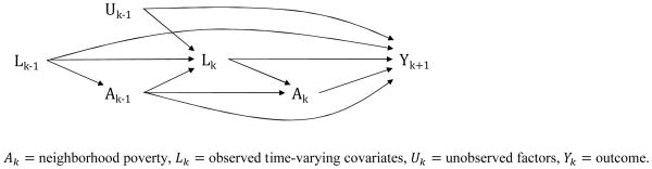
Hypothesized causal relationships between neighborhood poverty, time-varying covariates, and adolescent parenthood

A_k = neighborhood poverty, L_k = observed time-varying covariates, U_k = unobserved factors, Y_k = outcome.

To estimate the effects of neighborhood poverty on the risk of adolescent parenthood, the conventional regression approach involves fitting to the observed data a discrete-time logit model that conditions on confounder history. This model has form

$$\mathit{logit}\left(P(Y_k=1\mid k>7,{\overline{Y}}_{k-1}=0,{\overline{A}}_{k-1},{\overline{L}}_{k-1})\right)={\alpha }_0(k)+u({\overline{A}}_{k-1})+\epsilon ({\overline{L}}_{k-1}),$$ (5)

where α₀(k) are wave-specific intercept terms, u(Ā_{k − 1}) is a linear parametric function of neighborhood exposure history through wave k − 1, and ε(L̄_{k − 1}) is some parameterization of confounder history. For example, to estimate the parameters in Eq. 1 above, u(Ā_{k − 1}) includes main effects for the proportion of time lived in moderate- and high-poverty neighborhoods through wave k − 1, and the function ε(L̄_{k − 1}) typically includes main effects for the average of time-varying covariates from baseline through wave k − 1 (e.g., South and Crowder 2010), although many different specifications are possible.

This modeling strategy has two problems when time-varying confounders in L_k are affected by prior exposure to neighborhood poverty. First, Fig. 2a shows that conditioning on time-varying covariates affected by past treatment “controls away” the indirect effects of treatment that operate through these factors. Second, because conditioning on the common effect of two variables induces an association between them, models that include time-varying confounders as regressors may introduce a nuisance association between past treatment and unobserved determinants of the outcome (Greenland 2003; Pearl 2000). This problem, known as collider-stratification bias, is depicted in Fig. 2b. Thus, even when there is no unobserved confounding of neighborhood poverty, conventional discrete-time logit models fail to recover the treatment effects of interest.

Fig. 2.

Consequences of conditioning on time-varying confounders affected by past neighborhood context

A_k = neighborhood poverty, L_k = observed time-varying covariates, U_k = unobserved factors, Y_k = outcome.

Inverse Probability of Treatment Weighting

The method of inverse probability of treatment (IPT) weighting overcomes the problems outlined in the previous section (Robins et al. 2000). It involves computing a set of weights that, when applied to the observed data, generate a pseudo-population in which treatment at each time period is independent of prior (observed) time-varying covariates. Then, to estimate the effects of neighborhood poverty on adolescent parenthood, conventional discrete-time logit models that do not condition on time-varying confounder history are fit to the weighted observations.

The stabilized version of the IPT weight for the i^th subject at the k^th follow-up wave is given by

$${SW}_{ik}={\prod }_{t=1}^{k-1}\frac{P\left(A_t=a_{it}\mid {\overline{A}}_{t-1}={\overline{a}}_{i(t-1)},L_0=l_0\right)}{P\left(A_t=a_{it}\mid {\overline{A}}_{t-1}={\overline{a}}_{i(t-1)},{\overline{L}}_t={\overline{l}}_{it}\right)}.$$ (6)

The denominator of the weight is the probability that subject i is exposed to his/her observed level of neighborhood poverty at a given wave conditional on prior neighborhood exposures and time-varying covariates. The numerator, by contrast, is the conditional probability that a subject is exposed to his/her observed level of neighborhood poverty at each time period given neighborhood exposure history and covariates measured only at baseline. The stabilized IPT weight varies around 1 based on the degree to which neighborhood selection is influenced by time-varying factors. By weighting each person-wave observation by sw_ik, treatment assignment at each wave is balanced across prior levels of observed time-varying covariates. Figure 3 presents a stylized graph that illustrates the effect of IPT weighting: after the observed data are weighted by sw_ik, exposure to neighborhood poverty at each wave is independent of prior time-varying confounders. Conditioning on time-varying confounders, then, is no longer necessary, and conventional methods can be used with the weighted observations to estimate the neighborhood effects of interest.

Fig. 3.

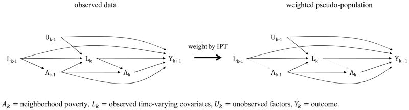
Stylized graph illustrating the effect of weighting by the inverse probability of treatment on the joint distribution of neighborhood poverty, time-varying covariates, and the outcome

A_k = neighborhood poverty, L_k = observed time-varying covariates, U_k = unobserved factors, Y_k = outcome.

The true stabilized IPT weights are unknown, but they can be estimated from data. For the three-level ordinal treatment, the denominator in Eq. 6 is estimated from an ordinal logistic regression model with form

$$\mathit{logit}\left(P(A_k>j\mid {\overline{A}}_{k-1},{\overline{L}}_k)\right)={\gamma }_{0j}(k)+{\gamma }_1{A}_{k-1}+{\gamma }_2{L}_0+{\gamma }_3{L}_{k-1}+{\gamma }_4{L}_k,j=1,\dots ,J-1$$ (7)

where γ_0j(k) is a wave-specific intercept term for the j^th cumulative logit. In Eq. 7, the level of neighborhood poverty to which a subject is exposed at each wave k is a function of neighborhood poverty at wave k − 1, covariates measured at baseline, and time-varying covariates measured at waves k and k − 1. The conditional probability in the numerator of the stabilized IPT weight is estimated from a similar model that constrains the coefficients on post-baseline covariates to zero. These models are estimated separately for black and nonblack subjects because prior research suggests that neighborhood selection processes differ by race (Charles 2003; Massey and Denton 1993; South and Deane 1993). Coefficient estimates from the treatment models and descriptive statistics for the treatment weights are reported in Parts A and B of the online supplement, respectively.

Below, regression-adjusted and IPT-weighted estimates of the parameters defined in Eqs. 1 and 2 are reported separately for blacks and nonblacks. Separate estimates for males and females are not reported because statistical tests provide no evidence that the effects of neighborhood poverty differ by gender. Regression-adjusted estimates come from models that condition on treatment history, baseline covariates, and post-baseline measurements of time-varying factors averaged across time. IPT-weighted estimates are computed by fitting discrete-time logit models to the weighted pseudo-population that condition on treatment history and covariates measured at baseline only. Equation 3 parameters are estimated from conventional discrete-time logit models that condition on treatment status at age 11, time-varying covariates measured concurrently with treatment, and baseline factors. Robust standard errors are computed for the IPT-weighted estimates to account for serial correlation induced by the weighting (Robins et al. 2000).

The IPT-weighted estimator is unbiased and consistent under the assumptions of no unmeasured confounders, no model misspecification, and positivity (Cole and Hernan 2008; Robins et al. 2000). Conventional regression estimators require these same assumptions and more. Specifically, they require the additional assumption that time-varying confounders are not affected by prior treatment. This assumption is almost certainly violated in observational studies of neighborhood effects. Although IPT weighting overcomes critical limitations of conventional regression modeling, the requisite assumptions for this method are not trivial.

First, if there are unobserved covariates that are risk factors for becoming an adolescent parent and for living in poor neighborhoods, then the IPT-weighted estimator is biased. I attempt to mitigate this problem by adjusting for a set of confounders that includes the most powerful joint predictors of neighborhood attainment and teen sexual behavior. Unobserved confounding, however, is still a possibility, since families may select different neighborhood contexts on the basis of unmeasured factors that affect the risk of adolescent parenthood. For example, subjects that live in poor neighborhoods may be at greater risk of adolescent parenthood regardless of where they reside because their parents are simply less ambitious, skilled, or intelligent when it comes to encouraging safe sexual activity. Since measures of these parental psychological factors are unavailable in the PSID, the IPT-weighted estimator would be upwardly biased if these characteristics are in fact confounders, indicating a higher risk of adolescent parenthood due to neighborhood poverty even when there is no such effect.

In some cases, experimental, quasi-experimental, or instrumental variable research designs that require less stringent assumptions about neighborhood selection can be used to overcome the problem of unobserved confounding in neighborhood effects research (e.g., Evans, Oates, and Schwab 1992; Goering and Feins 2003; Rosenbaum and Popkin 1991). However, for studies of time-dependent neighborhood effects, the high costs and logistical complexity associated with these methods likely preclude their implementation. Random assignment of subjects into different multiyear neighborhood exposure trajectories, rather than experimental or quasi-experimental manipulation of point-in-time contextual treatments, is prohibitively difficult. Absent some form of experimental control over neighborhood context across time, IPT weighting of observational data is the most defensible approach to estimating longitudinal neighborhood effects. Nevertheless, potential violations of the ignorability assumption on which this method is based necessitate caution when interpreting results.

Second, IPT-weighted estimation is biased if the models for selection into treatment are incorrectly specified. Experimentation with different treatment models, however, indicates that neighborhood-effect estimates are relatively invariant across a variety of specifications (see Part C of the online supplement for details). Third, IPT weighting requires the positivity assumption that nonzero treatment probabilities exist across all levels and combinations of prior confounders. This assumption is reasonable in the present context, since neighborhood choice is not formally restricted on the basis of economic or demographic characteristics, and descriptive analyses indicate that treatment occurs with positive probability across the support of several key confounders.

Censoring

Subjects who leave the study before they become parents or reach the end of follow-up are censored. Censoring can be problematic if subjects with certain characteristics are more likely to drop out of the study than others, so weights are used to adjust for potential nonrandom censoring based on observed covariates (Robins et al. 2000). The stabilized censoring weight for subject i at wave k is given by

$${cw}_{ik}={\prod }_{t=1}^{k-1}\frac{P\left(C_t=0\mid {\overline{C}}_{t-1}=0,{\overline{A}}_{t-1}={\overline{a}}_{i(t-1)},L_0=l_0\right)}{P\left(C_t=0\mid {\overline{C}}_{t-1}=0,{\overline{A}}_{t-1}={\overline{a}}_{i(t-1)},{\overline{L}}_t={\overline{l}}_{it}\right)},$$ (8)

where C_k is equal to 1 if a subject is censored at wave k and 0 otherwise. Pooled logistic regression models are used to estimate the probabilities in the weight (results not shown), and IPT-weighted estimates are computed using the product of the treatment and censoring weights.

Results

Sample Characteristics

Descriptive statistics for time-invariant covariates presented in Table 1 reveal substantial racial disparities on the majority of measured characteristics. For example, blacks are more likely than nonblacks to have young unmarried mothers and to come from families with low levels of parental education.

Table 1.

Descriptive statistics for time-invariant covariates in analyses of neighborhood effects on adolescent parenthood, Panel Study of Income Dynamics^a

Variable	Blacks (N=2669)	Nonblacks (N=3573)
Gender, %
Male	50.13	50.32
Female	49.87	49.68
Birth weight %
>= 5.5 lbs	91.08	94.57
< 5.5 lbs	8.92	5.43
Mother’s marital status at birth, %
Unmarried	48.48	7.30
Married	51.52	92.70
FU head’s education, %
Less than high school	43.42	21.80
High school graduate	29.30	24.71
At least some college	27.28	53.49
Mother’s age at birth, mean	24.74	26.51

^aStatistics reported for subjects who were not lost to follow-up before age 12.

Racial differences are also pronounced in Table 2, which contains descriptive statistics for time-varying covariates. Compared to nonblacks, blacks are more likely to live in a family that receives AFDC benefits, does not own a home, and has lower income. In addition, these statistics show considerable change over time in several family characteristics for both blacks and nonblacks. For example, at age 4, only about 33% of blacks live in families that own their residence, but by age 12, about 45% live with families that are homeowners. Similarly, from age 4 to 12, nonblacks become more likely to live in families that own a home.

Table 2.

Descriptive statistics for time-varying covariates in analyses of neighborhood effects on adolescent parenthood, Panel Study of Income Dynamics^a

Variable	Blacks (N=2669)		Nonblacks (N=3573)
	Age 4	Age 12	Age 4	Age 12
FU head’s marital status, %
Unmarried	41.06	48.71	9.57	14.50
Married	58.94	51.29	90.43	85.50
FU head’s employment status %
Unemployed	33.01	33.08	8.40	9.71
Employed	66.99	66.92	91.60	90.29
Public assistance receipt, %
Did not receive AFDC	76.47	78.16	95.27	95.83
Received AFDC	23.53	21.84	4.73	4.17
Homeownership, %
Did not own home	67.33	55.11	32.69	21.75
Owned home	32.67	44.89	67.31	78.25
FU income in $1000s, mean	15.70	17.13	30.13	37.10
FU head’s work hours, mean	27.58	27.30	41.46	40.26
FU size, mean	5.32	5.10	4.63	4.69
Cum. residential moves, mean	0.28	1.67	0.24	1.32

^aStatistics reported for subjects who were not lost to follow-up before age 12.

Table 3 describes the risk of adolescent parenthood by age and race. The probability of becoming a teen parent is substantially higher for blacks compared to nonblacks. At age 16, for example, the estimated probability of adolescent parenthood is about .05 for blacks and .01 for nonblacks. Overall, 511 blacks and 247 nonblacks, or about 19% and 7%, respectively, become adolescent parents.

Table 3.

Risk of adolescent parenthood by age (wave) and race, Panel Study of Income Dynamics^a

Age (wave)	Blacks				Nonblacks
	n	Yk	Ck	P(Yk)	n	Yk	Ck	P(Yk)
12 (k = 8)	2669	5	190	.002	3573	0	252	.000
13 (k = 9)	2474	6	193	.002	3321	2	251	.001
14 (k = 10)	2275	22	179	.010	3068	1	225	.000
15 (k = 11)	2074	47	164	.023	2842	15	226	.005
16 (k = 12)	1863	90	159	.048	2601	26	263	.010
17 (k = 13)	1614	99	155	.061	2312	49	216	.021
18 (k = 14)	1360	126	143	.093	2047	77	186	.038
19 (k = 15)	1091	116	975	.106	1784	77	1707	.043

^aY_k is an indicator for adolescent parenthood, P(Y_k) is the estimated probability of becoming an adolescent parent at wave k; and C_k represents censored observations.

Trajectories of Exposure to Neighborhood Poverty

Figure 4 illustrates neighborhood exposure trajectories from age 5 to 12 separately by race. Specifically, it presents sequence index plots, which use stacked line segments and differential shading to show how subjects move between levels of neighborhood poverty across time (Brzinsky-Fay et al. 2006). Each subject is represented by one horizontal line segment, and temporal changes in neighborhood exposure status are indicated with grayscale variations. These plots reveal extreme racial disparities in long-term exposure to neighborhood poverty, where blacks and nonblacks typically follow opposite treatment trajectories. The wide, light gray region at the top of the plot for nonblacks indicates that their modal treatment trajectory is sustained exposure to low-poverty neighborhoods, where about 40% experience long-term residence in neighborhoods of this type. The narrow, dark gray region at the bottom of this plot shows that only a small number of nonblacks, specifically, about 5%, experience sustained exposure to high-poverty neighborhoods from age 5 to 12. The plot for blacks, by contrast, shows that about 40% experience sustained exposure to high-poverty neighborhoods, and that only about 6% of blacks are continuously exposed to low-poverty neighborhoods.

Fig. 4.

Sequence index plots displaying trajectories of exposure to neighborhood poverty, Panel Study of Income Dynamics

Figure 4 also shows the extent of neighborhood mobility over time, as indicated by grayscale variation in the horizontal line segments. The regions that change from lighter to darker shades of gray show that many sample members move from neighborhoods with lower poverty rates to neighborhoods with higher poverty rates. The plots also show some upward neighborhood mobility for both blacks and nonblacks where line segments change from darker to lighter shades over time. Taken together, about 48% of blacks and about 42% of nonblacks experience at least one change in the level of neighborhood poverty to which they are exposed between age 5 and 12. About 25% of both groups move between treatment levels two or more times during the early life course.

Neighborhood Effects on Adolescent Parenthood

The first panel of Table 4 contains regression-adjusted and IPT-weighted estimates of the parameters defined in Eq. 1, which describe how the probability of adolescent parenthood changes with the cumulative proportion of time spent in moderate- and high-poverty neighborhoods. The regression-adjusted estimates control for observed confounding of neighborhood exposure status by conditioning on covariates measured at baseline and cross-time averages of time-varying covariates. These estimates indicate that exposure to neighborhood poverty has marginally significant effects on adolescent parenthood among both blacks and nonblacks. For blacks, the regression-adjusted estimates indicate that the odds of adolescent parenthood increase by about 60% with sustained exposure to either moderate-poverty (exp(0.467) = 1.595) or high-poverty (exp(0.455) = 1.576) neighborhoods, compared to continuous residence in low-poverty neighborhoods. Among nonblacks, the regression-adjusted estimates for Eq. 1 indicate that sustained exposure to moderate-poverty neighborhoods increases the odds of adolescent parenthood by 47% compared to continuous exposure to low-poverty neighborhoods; sustained exposure to high-poverty neighborhoods is estimated to increase the odds of adolescent parenthood by about 80%.

Table 4.

Effects of neighborhood (NH) poverty on the risk of adolescent parenthood, Panel Study of Income Dynamics^a

Model	Blacks (person-years=15420)				Nonblacks (person-years=21548)
	Reg-adjusted		IPT-weighted		Reg-adjusted		IPT-weighted
	LOR	SE	LOR	SE	LOR	SE	LOR	SE
Model 1
Cum. exposure
Low-poverty NH	ref	ref	ref	ref	ref	ref	ref	ref
Moderate-poverty NH	0.467	0.300	0.569	0.320†	0.383	0.269	0.460	0.265†
High-poverty NH	0.455	0.261†	0.601	0.266*	0.571	0.306†	0.829	0.297**
Model 2
Cum. exposure, childhood
Low-poverty NH	ref	ref	ref	ref	ref	ref	ref	ref
Moderate-poverty NH	0.167	0.329	0.103	0.355	0.129	0.345	0.249	0.364
High-poverty NH	0.152	0.319	0.212	0.339	−0.258	0.449	−0.138	0.478
Cum. exposure, adolescence
Low-poverty NH	ref	ref	ref	ref	ref	ref	ref	ref
Moderate-poverty NH	0.279	0.260	0.422	0.283	0.224	0.263	0.189	0.266
High-poverty NH	0.284	0.269	0.365	0.293	0.670	0.337*	0.790	0.341*
Model 3
Point exposure (age 11)
Low-poverty NH	ref	ref	-	-	ref	ref	-	-
Moderate-poverty NH	0.213	0.186	-	-	0.167	0.193	-	-
High-poverty NH	0.191	0.178	-	-	0.549	0.218*	-	-

^aLog odds ratios (LOR) and standard errors (SE) are combined estimates from 5 multiple imputation datasets

^†p<.10,

^*p<.05,

^**p<.01 and

^***p<.001 for two-sided tests of no effect.

IPT-weighted estimates of the log odds ratios in Eq. 1 indicate that neighborhood poverty has substantial and statistically significant effects on adolescent parenthood for both blacks and nonblacks. For blacks, the IPT-weighted estimates indicate that the odds of adolescent parenthood increase by about 75% with sustained exposure to moderate-poverty neighborhoods and by about 80% with sustained exposure to high-poverty neighborhoods, compared to continuous residence in low-poverty neighborhoods. For nonblacks, the IPT-weighted estimates indicate that sustained exposure to moderate-poverty neighborhoods increases the odds of adolescent parenthood by about 60% compared to extended residence in low-poverty neighborhoods, and sustained exposure to high-poverty neighborhoods is estimated to more than double the odds of early parenthood. Among nonblacks, IPT-weighted estimates for the effects of cumulative exposure to moderate- and high-poverty neighborhoods are about 20% and 40% larger, respectively, than corresponding regression-adjusted estimates. For blacks, the IPT-weighted estimates are more than 20% larger than corresponding regression-adjusted estimates. These differences suggest that conventional regression estimators understate the effects of neighborhood poverty on adolescent parenthood.

The second panel in Table 4 reports estimates from models that allow for different effects of cumulative exposure to neighborhood poverty during childhood versus adolescence. The IPT-weighted estimates have large standard errors, indicating that the available data allow only imprecise estimates of neighborhood effects by developmental stage, and Wald tests (not reported) indicate that observed differences in the effects of exposure to neighborhood poverty during childhood versus adolescence are not statistically significant at conventional thresholds. Nevertheless, these results are at least suggestive of timing differences, where exposure during adolescence appears to be more consequential than exposure during childhood.

For example, among nonblacks, the IPT-weighted estimates indicate that cumulative exposure to high-poverty neighborhoods during adolescence has a significant positive effect on the probability of becoming an adolescent parent. The estimated effects of childhood exposure to neighborhood poverty, by contrast, are much smaller and not statistically significant. Similarly, for blacks, the IPT-weighted estimates for cumulative exposure to neighborhood poverty during adolescence are considerably larger than those for exposure during childhood, although none of these estimates are statistically significant. Thus, while point estimates for Eq. 2 should be interpreted with caution given their high variability, these results suggest that exposure to neighborhood poverty during adolescence may have a more notable effect on the risk of becoming a teen parent than exposure earlier during childhood.

The lower panel of Table 4 reports regression-adjusted estimates based on point-in-time measures of neighborhood poverty taken at age 11. As expected, they are smaller than IPT-weighted estimates based on longitudinal measures of neighborhood poverty. For blacks, they are about a third the size of IPT-weighted estimates for the effects of cumulative exposure to neighborhood poverty. Among nonblacks, regression-adjusted estimates with point-in-time measures are also much smaller than estimates obtained via IPT weighting and longitudinal measurement of neighborhood poverty. These differences underscore the importance of accounting for both longitudinal exposure trajectories and dynamic neighborhood selection.

Discussion

The effect of growing up in disadvantaged neighborhoods on adolescent parenthood is central to understanding poverty and the reproduction of inequality over time. Past research on this issue, however, neglects duration and timing of exposure to poor neighborhoods and does not properly address the dynamic selection process that defines how children come to live in different neighborhood environments throughout the early life course. This inattention to longitudinal exposure patterns and dynamic neighborhood selection may underlie the mixed results of previous research, wherein many studies suggest only a minimal influence for neighborhood context on adolescent parenthood (Brooks-Gunn et al. 1993; Galster et al. 2007; Ginther et al. 2000; Thornberry et al. 1997).

The present study investigates how the impact of neighborhood poverty on adolescent parenthood depends on the duration and timing exposure. It measures neighborhood context once per year from early childhood through late adolescence and uses novel methods that properly adjust for dynamic neighborhood selection on observed covariates. Unlike conventional methods, the IPT weighting approach employed here does not remove the indirect effects of neighborhood poverty that operate through time-varying characteristics of the family and is therefore capable of estimating the total effects of different longitudinal exposure patterns. These methods are not without limitations, but they allow for unbiased and consistent estimation of neighborhood effects under assumptions that are less stringent than those required for conventional regression.

The results of this study indicate that long-term exposure to poor neighborhoods substantially increases the risk of adolescent parenthood, and that exposure to neighborhood poverty during adolescence may be more consequential than exposure earlier during childhood. Estimates for the effect of sustained exposure to poor neighborhoods are also considerably larger than estimates based on point-in-time measurements of neighborhood context, and the different estimates obtained from IPT weighting versus conventional regression indicate that effects of neighborhood poverty operate indirectly through measured time-varying characteristics of family, such as parental employment, income, and marital status. Taken together, these findings demonstrate that it is critically important to account for longitudinal exposures to neighborhood poverty and for the dynamic selection and feedback mechanisms that structure how neighborhood poverty impacts sexual behavior during adolescence. Studies that rely on static measures of neighborhood context and conventional regression methods risk understating the full impact of neighborhood poverty. In addition, these results complicate the conceptual separation of neighborhood and family effects on child development in ecological socialization theories (e.g., Leventhal and Brooks-Gunn 2000; Small and Newman 2001). Neighborhood effects are mediated by family effects, and vice versa (Sampson et al. 2008; Sharkey and Elwert 2011; Wodtke et al. 2011).

The evidence presented here demonstrates that a temporal framework is essential for understanding neighborhood effects. Many families move between different neighborhood environments or remain in communities whose social composition changes over time, raising important questions about effects of different longitudinal exposures to neighborhood poverty. In contrast to previous research, the time-dependent effects of neighborhood poverty reported in this study are more consistent with core theories that motivate research on the consequences of spatially concentrated poverty (Wilson 1987, 1996), with research on neighborhood attainment and mobility (Sampson and Sharkey 2008), and with developmental perspectives on the reproduction of inequality (Duncan et al. 1998). To advance research on the processes through which poverty is generated and maintained, a more complete integration of ecological and temporal perspectives on spatial stratification is needed.

While this study addresses the lack of research on the effects of neighborhood poverty within a temporal framework, it nevertheless suffers from several limitations. First, it focuses on a single outcome, adolescent parenthood, which represents the final stage in a series of decisions about engaging in sexual intercourse, using contraception, and carrying a pregnancy to term. Investigating how neighborhood context influences the proximate determinants of fertility would provide further insight into the social processes through which neighborhood effects operate.

Second, although the PSID is arguably the most comprehensive source of longitudinal information on neighborhood context, this study still lacks the data needed to precisely estimate time-dependent effects of neighborhood poverty. Additional data must be collected to better understand the temporal dimensions of neighborhood effects. Future studies should experiment with new procedures to gather information on neighborhood exposure histories and prior time-varying confounders that are not as costly and difficult as following a cohort of children for more than 15 years. For example, large cross-sectional surveys might consider adapting retrospective life history calendars to record past residential locations (Axinn et al. 1999).

Finally, this study does not investigate the specific mechanisms, such as social isolation, collective disorganization, and resource deprivation, thought to transmit the effects of concentrated neighborhood poverty to adolescent parenthood. While such an analysis is beyond the scope of the present study, it is nevertheless critically important for understanding the social processes through which the local environment shapes the sexual behavior of individuals during the early life course.

The impact of sustained exposure to neighborhood poverty on adolescent parenthood identified in this study suggests that neighborhood-effects research is essential to understanding the reproduction of inequality. As social scientists increasingly grapple with the role of time in spatial stratification, future studies using new and more flexible methods may find contextual effects on other outcomes to be even more important than previously documented. In order to advance knowledge of the causes and consequences of inequality, rigorous integration of social theory and quantitative empirical practice regarding the temporal dimensions of social context is crucial.

References

- Anderson E. Neighborhood effects on teenage pregnancy. In: Jencks C, Peterson PE, editors. The urban underclass. Washington, DC: Brookings; 1991. pp. 375–398. [Google Scholar]
- Axinn WG, Pearce LD, Ghimire D. Innovations in life history calendar applications. Social Science Research. 1999;28:243–264. [Google Scholar]
- Brewster KL. Race differences in sexual-activity among adolescent women: The role of neighborhood characteristics. American Sociological Review. 1994;59:408–424. [Google Scholar]
- Brewster KL, Billy JOG, Grady WR. Social context and adolescent behavior: The impact of community on the transition to sexual activity. Social Forces. 1993;71:713–740. [Google Scholar]
- Brooks-Gunn J, Duncan GJ, Aber JL. Neighborhood poverty (vol. 1): Context and consequences for children. New York: Russell Sage; 1997. [Google Scholar]
- Brooks-Gunn J, Duncan GJ, Klebanov PK, Sealand N. Do neighborhoods influence child and adolescent development? American Journal of Sociology. 1993;99:353–395. [Google Scholar]
- Browning CR, Leventhal T, Brooks-Gunn J. Neighborhood context and racial differences in early adolescent sexual activity. Demography. 2004;41:697–720. doi: 10.1353/dem.2004.0029. [DOI] [PubMed] [Google Scholar]
- Browning CR, Leventhal T, Brooks-Gunn J. Sexual initiation in early adolescence: The nexus of parental and community control. American Sociological Review. 2005;41:697–720. [Google Scholar]
- Brzinsky-Fay C, Kohler U, Luniak M. Sequence analysis with stata. The Stata Journal. 2006;6:435–460. [Google Scholar]
- Charles CZ. The dynamics of racial residential segregation. Annual Review of Sociology. 2003;29:167–207. [Google Scholar]
- Cole SR, Hernan MA. Constructing inverse probability of treatment weights for marginal structural models. American Journal of Epidemiology. 2008;168:656–664. doi: 10.1093/aje/kwn164. [DOI] [PMC free article] [PubMed] [Google Scholar]
- Cook TD, Shagle SC, Degirmencioglu SM. Capturing social process for testing mediational models of neighborhood effects. In: Brooks-Gunn J, Duncan GJ, Aber JL, editors. Neighbohood poverty (vol. 2): Policy implications in studying neighborhoods. New York: Russell Sage; 1997. pp. 94–119. [Google Scholar]
- Darling N, Steinberg L. Community influences on adolescent achievement and deviance. In: Brooks-Gunn J, Duncan GJ, Aber JL, editors. Neighborhood poverty (vol. 2): Policy implications in studying neighborhoods. New York: Russell Sage; 1997. pp. 120–131. [Google Scholar]
- Duncan GJ, Yeung WJ, Brooks-Gunn J, Smith JR. How much does childhood poverty affect the life chances of children? American Sociological Review. 1998;63:406–423. [Google Scholar]
- Evans WN, Oates WE, Schwab RM. Measuring peer group effects: A study of teenage behavior. Journal of Political Economy. 1992;100:966–991. [Google Scholar]
- Fernandez RM, Su C. Space in the study of labor markets. Annual Review of Sociology. 2004;30:545–569. [Google Scholar]
- Galster G, Marcotte DE, Mandell M, Wolman H, Augustine N. The influence of neighborhood poverty during childhood on fertility, education, and earnings outcomes. Housing Studies. 2007;22:723–751. [Google Scholar]
- Ginther D, Haveman R, Wolfe B. Neighborhood attributes as determinants of children’s outcomes: How robust are the relationships? Journal of Human Resources. 2000;35:603–642. [Google Scholar]
- Goering JM, Feins JD. Choosing a better life? Evaluating the Moving to Opportunity social experiment. Washington, DC: Urban Institute Press; 2003. [Google Scholar]
- Greenland S. Quantifying biases in causal models: Classical confounding vs collider-stratification bias. Epidemiology. 2003;14:300–306. [PubMed] [Google Scholar]
- Harding DJ. Counterfactual models of neighborhood effects: The effect of neighborhood poverty on dropping out and teenage pregnancy. American Journal of Sociology. 2003;109:676–719. [Google Scholar]
- Harding DJ. Collateral consequences of violence in disadvantaged neighborhoods. Social Forces. 2009;88:757–784. doi: 10.1353/sof.0.0281. [DOI] [PMC free article] [PubMed] [Google Scholar]
- Harding DJ. Living the drama: Community, conflict, and culture among inner-city boys. Chicago: University of Chicago Press; 2010. [Google Scholar]
- Hayes CD. Risking the future: Adolescent sexuality, pregnancy, and childbearing. Washington, DC: National Academy Press; 1987. [PubMed] [Google Scholar]
- Heckman JJ. Skill formation and the economics of investing in disadvantaged children. Science. 2006;312:1900–1901. doi: 10.1126/science.1128898. [DOI] [PubMed] [Google Scholar]
- Iceland J, Scopilliti M. Immigrant residential segregation in US metropolitan areas, 1990–2000. Demography. 2008;45:79–94. doi: 10.1353/dem.2008.0009. [DOI] [PMC free article] [PubMed] [Google Scholar]
- Jargowsky PA. Poverty and place: Ghettos, barrios, and the American city. New York: Russell Sage; 1997. [Google Scholar]
- Jencks C, Mayer SE. The social consequences of growing up in a poor neighborhood. In: Lynn LE, McGreary MGH, editors. Inner-city poverty in the United States. Washington, DC: National Academy Press; 1990. pp. 111–186. [Google Scholar]
- Leventhal T, Brooks-Gunn J. The neighborhoods they live in: The effects of neighborhood residence on child and adolescent outcomes. Psychological Bulletin. 2000;126:309–337. doi: 10.1037/0033-2909.126.2.309. [DOI] [PubMed] [Google Scholar]
- Massey DS, Denton NA. American apartheid: Segregation and the making of the underclass. Cambridge, MA: Harvard University Press; 1993. [Google Scholar]
- Maynard RA. Kids having kids: A special report on the costs of adolescent childbearing. New York: Robin Hood Foundation; 1996. [Google Scholar]
- McLanahan S, Percheski C. Family structure and the reproduction of inequalities. Annual Review of Sociology. 2008;34:257–276. [Google Scholar]
- Nock SL. The Consequences of Premarital Fatherhood. American Sociological Review. 1998;63:250–263. [Google Scholar]
- Pearl J. Causality: Models, reasoning, and inference. Cambridge: Cambridge University Press; 2000. [Google Scholar]
- Quillian L. How long are exposures to poor neighborhoods? The long-term dynamics of entry and exit from poor neighborhoods. Population Research and Policy Review. 2003;22:221–249. [Google Scholar]
- Robins J. A new approach to causal inference in mortality studies with a sustained exposure period—Application to control of the healthy worker survivor effect. Mathematical Modeling. 1987;7:1393–1512. [Google Scholar]
- Robins JM, Hernan MA, Brumback B. Marginal structural models and causal inference in epidemiology. Epidemiology. 2000;11:550–560. doi: 10.1097/00001648-200009000-00011. [DOI] [PubMed] [Google Scholar]
- Rosenbaum JE, Popkin SJ. Employment and earnings of low-income blacks who move to middle-class suburbs. In: Jencks C, Peterson P, editors. The Urban Underclass. Washington, DC: Brookings Institution Press; 1991. pp. 342–356. [Google Scholar]
- Rubin DB. Multiple imputation for nonresponse in surveys. New York: J. Wiley & Sons; 1987. [Google Scholar]
- Sampson RJ. How do communities undergird or undermine human development? Relevant contexts and social mechanisms. In: Booth A, Crouter N, editors. Does it take a village? Community effects on children, adolescents, and families. Mahwah, NJ: Erlbaum; 2001. pp. 3–30. [Google Scholar]
- Sampson RJ, Sharkey P. Neighborhood selection and the social reproduction of concentrated racial inequality. Demography. 2008;45:1–29. doi: 10.1353/dem.2008.0012. [DOI] [PMC free article] [PubMed] [Google Scholar]
- Sampson RJ, Sharkey P, Raudenbush SW. Durable effects of concentrated disadvantage on verbal ability among African-American children. Proceedings of the National Academy of Sciences. 2008;105:845–852. doi: 10.1073/pnas.0710189104. [DOI] [PMC free article] [PubMed] [Google Scholar]
- Sharkey P, Elwert F. The legacy of disadvantage: Multigenerational neighborhood effects on cognitive ability. American Journal of Sociology. 2011;116:1934–1981. doi: 10.1086/660009. [DOI] [PMC free article] [PubMed] [Google Scholar]
- Small ML, Newman K. Urban poverty after The Truly Disadvantaged: The rediscovery of the family, the neighborhood, and culture. Annual Review of Sociology. 2001;27:23–45. [Google Scholar]
- South SJ, Baumer EP. Community effects on the resolution of adolescent premarital pregnancy. Journal of Family Issues. 2001;22:1025–1043. [Google Scholar]
- South SJ, Crowder KD. Escaping distressed neighborhoods: Individual, community, and metropolitan influences. American Journal of Sociology. 1997;102:1040–1084. [Google Scholar]
- South SJ, Crowder KD. Neighborhood effects on family formation: Concentrated poverty and beyond. American Sociological Review. 1999;64:113–132. [Google Scholar]
- South SJ, Crowder KD. Neighborhood poverty and nonmarital fertility: Spatial and temporal dimensions. Journal of Marriage and Family. 2010;72:89–104. doi: 10.1111/j.1741-3737.2009.00685.x. [DOI] [PMC free article] [PubMed] [Google Scholar]
- South SJ, Deane GD. Race and residential mobility: Individual determinants and structural constraints. Social Forces. 1993;72:147–167. [Google Scholar]
- Speare A, Goldscheider FK. Effects of marital status change on residential mobility. Journal of Marriage and the Family. 1987;49:455–464. [Google Scholar]
- Sucoff CA, Upchurch DM. Neighborhood context and the risk of childbearing among metropolitan-area black adolescents. American Sociological Review. 1998;63:571–585. [Google Scholar]
- Thornberry TP, Smith CA, Howard GJ. Risk factors for teenage fatherhood. Journal of Marriage and the Family. 1997;59:505–522. [Google Scholar]
- Timberlake JM. Racial and ethnic inequality in the duration of children’s exposure to neighborhood poverty and affluence. Social Problems. 2007;54:319–342. [Google Scholar]
- Vere JP. The perils of father-reported fertility data for household labour supply models. Population Studies. 2008;62:235–243. doi: 10.1080/00324720801904816. [DOI] [PubMed] [Google Scholar]
- Wilson WJ. The truly disadvantaged: The inner city, the underclass, and public policy. Chicago: University of Chicago Press; 1987. [Google Scholar]
- Wilson WJ. When work disappears: The world of the new urban poor. New York: Vintage Books; 1996. [Google Scholar]
- Wodtke GT, Harding DJ, Elwert F. Neighborhood effects in temporal perspective: The impact of long-term exposure to concentrated disadvantage on high school graduation. American Sociological Review. 2011;76:713–736. doi: 10.1177/0003122411420816. [DOI] [PMC free article] [PubMed] [Google Scholar]
- Yinger J. Closed doors, opportunities lost: The continuing costs of housing discrimination. New York: Russell Sage; 1995. [Google Scholar]
Associated Data
This section collects any data citations, data availability statements, or supplementary materials included in this article.