Non-Invasive Quantification of Absolute Cerebral Blood Volume During Functional Activation Applicable to the Whole Human Brain

Abstract

Purpose

Cerebral blood volume (CBV) changes in many diverse pathologic conditions, and in response to functional challenges along with changes in blood flow, blood oxygenation, and the cerebral metabolic rate of oxygen. The feasibility of a new method for non-invasive quantification of absolute cerebral blood volume that can be applicable to the whole human brain was investigated.

Methods

Multi-slice data were acquired at 3 T using a novel inversion recovery echo planar imaging (IR-EPI) pulse sequence with varying contrast weightings and an efficient rotating slice acquisition order, at rest and during visual activation. A biophysical model was used to estimate absolute cerebral blood volume at rest and during activation, and oxygenation during activation, on data from 13 normal human subjects.

Results

Cerebral blood volume increased by 21.7% from 6.6±0.8 mL/100 mL of brain parenchyma at rest to 8.0±1.3 mL/100 mL of brain parenchyma in the occipital cortex during visual activation, with average blood oxygenation of 84±2.1% during activation, comparing well with literature.

Conclusion

The method is feasible, and could foster improved understanding of the fundamental physiological relationship between neuronal activity, hemodynamic changes, and metabolism underlying brain activation; complement existing methods for estimating compartmental changes; and potentially find utility in evaluating vascular health.

Cerebral blood volume (CBV) is a fundamental physiological parameter defined as milliliters (mL) of blood per 100 mL of brain parenchyma (mL/100 mL). CBV changes in many diverse pathologic conditions such as Alzheimer’s disease (1,2), brain tumors (3), acute stroke (4), arteriovenous malformations (5), schizophrenia, depression, and substance abuse (6). Such changes can precede observation of abnormalities in structural imaging (7), and could become valuable early markers of disease. CBV also changes in response to functional challenges along with changes in cerebral blood flow (CBF), blood oxygenation, and CMRO₂, the cerebral metabolic rate of oxygen (8–11). CBV changes localize very well with neural activity (12), providing an important contrast mechanism for functional brain imaging (13–15).

Blood oxygenation level-dependent (BOLD) functional magnetic resonance imaging (MRI) is primarily sensitive to changes in deoxyhemoglobin concentration with activation; and calibrated functional MRI aims to dissociate changes in CMRO₂ from changes in CBF and CBV (16,17). CBV and oxygenation changes in arterial, capillary, and venous compartments impact BOLD differently. Many studies have assumed that CBV is related to CBF^α (16,18–22), with α = 0.38 based on total CBV in monkeys (23), although α may differ across functional challenges, brain regions, and species (17,23–27), i.e. α = 0.23 based on venous CBV in humans (28). Venous CBV has the largest impact on BOLD due to large oxygenation changes on the venous side (29). Optical measurements in animals indicate a complicated mechanism involving small venous CBV changes (30) as also supported by MRI in animals (31,32) and humans (28); and oxygenation changes have even been shown on the arterial side (30,33). Significant capillary CBV changes have also been suggested (30,34–36), given that capillaries are the major source of oxygen extraction and closer to activation site (36). Compartmental CBV dynamics could also change with stimulus duration (typically much shorter in optical compared to functional MRI experiments).

Non-invasive MRI approaches for CBV quantification in humans include vascular space occupancy (VASO) for relative total CBV assuming a baseline CBV (13); inflow VASO (iVASO) and iVASO with dynamic subtraction (DS) for absolute arteriolar CBV (37–39); and venous refocusing for volume estimation (VERVE) for relative venous CBV (40). A biophysical model has also been used for quantification of absolute total CBV in one (41) or five slices (42). Our proposed method is similarly based on an inversion recovery acquisition and a biophysical model for absolute quantification of total CBV in the steady-state, however, with the following changes. Extended slice coverage was enabled by efficient rotating slice acquisition over a balanced and consistent range of inversion times (TIs). Steady-state was maintained throughout varying inversion and recovery durations by non-selective saturation and spoiler gradients. The biophysical model was also modified to attribute enhanced tissue relaxation to deoxygenated blood. The current method with sensitivity to total CBV and oxygenation changes could also complement existing arterial or venous CBV weighted methods to improve our understanding of compartmental changes in different brain regions, stimulus types, and durations in humans.

METHODS

Pulse Sequence

The pulse sequence is illustrated in Figure 1a. Non-selective adiabatic inversion is followed by a gradient spoiler. Acquisition of multiple slices begins at TI, followed by another gradient spoiler, global saturation, and a final spoiler to maintain steady-state by enforcing identical recovery durations for all slices (using multidirectional gradient cycling (43)).

FIG. 1.

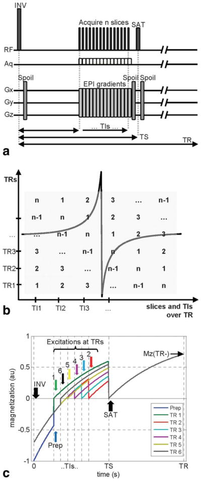
a: Multi-slice pulse sequence diagram. INV: inversion, SAT: saturation, Spoil: gradient spoiler, TI: inversion time, TS: saturation time, TR: repetition time, Aq: acquisition. Slices are acquired using standard EPI with EPI gradients consisting of slice selection (Gz), blipped (Gy), and alternating (Gx) components. Spoiler gradients can be on one, two, or three axes (following the multidirectional gradient cycling scheme proposed by Lu et al. (43)) during different TRs. b: Slice acquisition order within each TR and over successive TRs, depicted for n slices acquired at n TI values. c: Longitudinal signal evolution over multiple TRs, signal simulated for the first slice of a 6-slice acquisition with one preparation pulse to achieve steady-state (blue) and TR = 3 s, TIs = (0.4, 0.54, 0.68, 0.82, 0.96, 1.1)s, TS = 1.5 s, T₁ = 1.2 s. Note that these parameters were selected for clarity of the display and differ from actual experimental parameters.

For an inversion-recovery experiment with TI (s), repetition time (TR) (s) and longitudinal relaxation time constant T₁ (s), longitudinal magnetization M_z at time TI is:

$$M_z({\text{TI}}^{-})=M_0(1-2exp(-\text{TI}/T_1)+exp(-\text{TR}/T_1))$$ [1]

where M₀ is the equilibrium magnetization (A/m) established by the external magnetic field B₀ (T). For our multi-slice acquisition with an additional saturation pulse at time TS (saturation time, s) and the described spoiling scheme, longitudinal magnetization M_z at time TI is:

$$M_z({\text{TI}}^{-})=M_0(1-2exp(-\text{TI}/T_1)+exp(-(\text{TR}-\text{TS}+\text{TI})/T_1))$$ [2]

The slice acquisition order is depicted in Figure 1b, and consists of shifting the order of slices over successive TRs such that the same range of TI values is covered for each slice. In the first TR, acquisition begins with the first slice at the first TI, and continues with the second slice at the second TI, third slice at the third TI …, until the last slice is acquired at the last TI. In the second TR, the second slice is acquired in the first TI, the third slice in the second TI …, after the last slice, acquisition continues with the first slice at the last TI. This rotating acquisition continues until each slice is acquired at each TI. While a different number of TIs and slices could be accommodated with corresponding modifications to the signal equation, in this study the number of TIs equals the number of slices, and the acquisition is completed when the number of TRs equals the number of TIs and slices.

Longitudinal signal evolution over time is simulated for a sample slice of a multi-slice acquisition over multiple TRs in Figure 1c. At time t = 0 in each TR, all magnetization is inverted non-selectively, and magnetization recovers until excitation at time t = TI. Following the excitation, magnetization begins recovering from 0 toward its equilibrium value, until non-selective saturation at time t = TS. Following the non-selective saturation, magnetization begins recovering from 0 to its equilibrium value until non-selective inversion in the next TR. Note that steady-state is established after the first TR period, and different TI values for each slice are acquired in successive TRs. The signal vs. TI curve differs between rest and activation conditions, and is used for quantification as outlined below.

Biophysical Model

Consider a voxel containing CSF and brain parenchyma, where CBV is the blood fraction in brain parenchyma. MR signal magnitude from such a voxel includes contributions from each compartment:

$$S=K.\mathit{abs}(S_{\text{CSF}}+S_{\text{OBV}}+S_{\text{DBV}}+S_{\text{TISSUE}})$$ [3]

where K is a calibration factor accounting for equilibrium magnetization with transmit and receive sensitivity effects assuming uniform coil profiles and M₀ (a.u.). OBV is the oxygenated blood volume, while DBV is the deoxygenated blood volume where deoxyhemoglobin-containing blood creates mesoscopic magnetic field inhomogeneity-induced signal decay in surrounding tissues (44–46). In the resting brain, arteriolar compartments are nearly fully oxygenated. However, note that OBV and DBV are functional definitions. In the activated brain, OBV and DBV may correspond to different physical parts of the blood vessel network, i.e. OBV including a significant portion of the capillary compartment if capillaries become nearly fully oxygenated during activation. Each compartment contributes to signal according to its volume fraction F in the voxel (dimensionless), water proton density C (dimensionless), effective transverse relaxation time constant $T_2^{\ast }$ (s), and longitudinal magnetization, M_z, at the time of excitation including longitudinal relaxation effects. For the proposed pulse sequence, using M_z as defined in Eq. [2], signal at TI is:

$$S_{\mathrm{i}}(\text{TI})=F_{\mathrm{i}}.C_{\mathrm{i}}.M_{z,\mathrm{i}}({\text{TI}}^{-}).exp(-\text{TE}/T_{2,\mathrm{i}}^{\ast })$$ [4]

for i = CSF, OBV, and DBV, where TE is the echo time (s), with:

$$M_{z,\mathrm{i}}({\text{TI}}^{-})=1-2exp(-\text{TI}/T_{1,\mathrm{i}})+exp(-(\text{TR}-\text{TS}+\text{TI})/T_{1,\mathrm{i}})$$ [5]

for i = CSF, OBV, DBV, and TISSUE. Extravascular tissue signal is modified by the influence of deoxygenated blood and its oxygenation level (44–46), as follows:

$$S_{\text{TISSUE}}(\text{TI})=F_{\text{TISSUE}}.C_{\text{TISSUE}}.M_{z,\text{TISSUE}}({\text{TI}}^{-}).exp(-\text{TE}/T_{2,\text{TISSUE}}-F_{\text{DBV}}.f(Y_{\text{DBV}},\text{Hct}))$$ [6]

$$f(Y_{\text{DBV}},\text{Hct})=\frac{1}{3}\underset{0}{\overset{1}{\int }}(2+u)\sqrt{1-u}\times \left(\frac{1-J_0(2.\mathrm{\gamma }.B_0.\mathrm{\pi }.\mathrm{\Delta }\mathrm{\chi }.\text{TE}.\text{Hct}.(1-Y_{\text{DBV}}).u)}{u^2}\right)\mathrm{d}u$$ [7]

where T_2,TISSUE is the transverse relaxation time constant (s), F_DBV is the fraction of DBV in the voxel (%), Y_DBV is the DBV oxygenation fraction (%), Hct is the microvascular hematocrit estimate (%), J₀ is the zero-order Bessel function, γ is the gyromagnetic ratio (42.576 MHz/T), Δx is the susceptibility difference between fully oxygenated and deoxygenated blood (ppm). Note that, consistent with the original theory and utilizations in Refs. (44–47), Eqs. [6 and 7] attribute the susceptibility induced enhanced relaxation in tissue to DBV, as opposed to total CBV (41,42,47); and represent the complete solution, as opposed to asymptotic approximations (41,42,47). The total blood volume, CBV, is:

$$\text{CBV}=(F_{\text{OBV}}+F_{\text{DBV}})/(1-F_{\text{CSF}})$$ [8]

T₁ of blood varies slightly with hematocrit and blood oxygenation, decreasing with increased hematocrit and reduced oxygenation (48,49). These dependencies are typically (incorrectly) assumed to be negligible at 3 T, but small errors can effect quantification (50,51), and have been included in the model:

$$T_{1,\text{blood}}(Y_{\mathrm{b}},\text{HCt})=1/(a.\text{Hct}+b.Y_{\mathrm{b}}+c.Y_{\mathrm{b}}.\text{Hct}+d)$$ [9]

where Y_b is the average blood oxygenation fraction (%, Y_b = 98% for OBV, Y_b = Y_DBV for DBV, Y_b = (Y_OBV F_OBV+Y_DBV F_DBV)/(F_OBV+F_DBV) for CBV), a = 2.4084 (s⁻¹), b = 0.708 (s⁻¹), c = −1.9998 (s⁻¹), d = −0.2892 (s⁻¹), based on interpolation of published results (48,49,51). For instance, commonly used blood T₁s of 1624–1627 ms correspond to Y_b = 81% (average of measurements at arterial Y_b = 92% and venous Y_b = 69%), and T₁ of 1612 ms corresponds to Y_b = 77%, approximately, both at Hct of 42% (average of male and female macrovascular Hct). Considering a lower microvascular Hct of 37.4% (85% of macrovascular Hct), blood T₁s of 1747 ms and 1703 ms correspond to arterial Y_b = 98% and venous Y_b = 61%, respectively (51).

$T_2^{\ast }$ varies with macroscopic field inhomogeneities (i.e., magnet imperfections, air interfaces…) causing signal loss and spatial distortions; however, these static effects are not expected to change with brain activation and provide no physiologic information of interest. $T_2^{\ast }$ of blood also varies with hematocrit and blood oxygenation, decreasing with increasing hematocrit and decreasing oxygenation (52,53). At 3 T under physiological conditions (52):

$$T_{2,\text{blood}}^{\ast }(Y_{\mathrm{b}},\text{Hct})=1/(a^{\ast }(\text{Hct})+b^{\ast }(\text{Hct}).(1-Y_{\mathrm{b}})+c^{\ast }(\text{Hct}).{(1-Y_{\mathrm{b}})}^2)$$ [10]

where a*, b*, and c* depend on hematocrit. For Hct = 34%, (females, for 85% of macrovascular Hct = 40%) a*: 16.1957 (s⁻¹), b* = 36.5348 (s⁻¹), c* = 91.3478 (s⁻¹), and for Hct = 38.25% (males, for 85% of macrovascular Hct = 45%) a* = 16.75 (s⁻¹), b* = 37.625 (s⁻¹), c* = 103.1 (s⁻¹) based on interpolation of published results (51,52). For example, $T_2^{\ast }$ of blood is approximately 58 ms at Y_b = 98%, and 22 ms at Y_b = 61%, at an intermediate Hct = 36.125% (average of male and female microvascular Hct).

Functional challenges influence the voxel signal S through changes in compartment fractions F (altering the weight of each compartment according to Eq. [4], and tissue transverse relaxation according to Eq. [6]) as well as blood oxygenation Y_b (altering the transverse relaxation of both tissue and blood according to Eqs. [7 and 10], and to a lesser extent the longitudinal relaxation of blood according to Eqs. [5 and 9]). A slight curve shift occurs upon stimulation (41,42), and CBV (Eq. [8]) can be estimated by fitting the fractional signal change between rest and activation, (S_act−S_rest)/S_rest, over multiple TI times.

MRI Experiments

Thirteen normal volunteers provided written informed consent and participated in this Yale University Institutional Review Board approved, Health Insurance Portability, and Accountability Act compliant study (five females, mean age±sd: 31.5±6.5 years, range: 24–42 years). Experiments were performed on a 3 T whole body scanner (Tim Trio, Siemens Medical Systems, Erlangen Germany) with a 32-channel receive-only phased-array head coil and body coil transmission. 3D high-resolution (MPRAGE, 1 mm isotropic, 176 × 202 × 179 mm³ field of view (FOV), TE/TR = 2/2530 ms) acquisition was followed by multi-slice 2D high-resolution (FLASH, 1 mm in-plane, TE/TR = 2.5/300 ms), T₁ mapping and CBV sequences with the same slice prescription. Multi-slice prescriptions consisted of 20 transverse slices covering the whole brain including the calcarine fissure with 4 mm slice thickness and 2 mm gap in the current study; however, the number of slices can be adjusted according to the desired application with corresponding changes in the number of TIs and acquisition time as described in the Pulse Sequence section. Figure 2 depicts the typical slice prescription. All inversion and saturation pulses were applied non-selectively. CBV sequence parameters were: TE/TS/TR = 11 ms/1.2 s/3 s, gradient-echo EPI, 192 × 256 mm² FOV, 4 × 4 mm² in-plane. TI values were acquired in 3 sets of 20 TIs at the following values:

$$\mathbf{TIs}(n,s)={\text{TI}}_{\text{start}}+(n-1)\times {\text{TI}}_{\text{shift}}+(s-1)\times {\text{TI}}_{\text{gap}}$$ [11]

where TI_start = 400 ms, TI_shift = 13 ms, TI_gap = 38.51 ms, n = 1–3, and s = 1–20, covering the TI range of 400–1158 ms with 13 ms resolution. Figure 3 shows sample images at different TIs. For T₁ mapping, TI values covering the TI range of 120–2400 ms were acquired in steps of 120 ms with TE/TS/TR = 11 ms/2.5 s/6 s and three repetitions. Stimulation consisting of a full-field black-and-white flashing checkerboard (frequency 10Hz) was presented on a back-projection screen viewed from a mirror mounted on the head coil. CBV data were acquired during presentation of a block paradigm of three OFF/ON cycles programmed in Eprime (Psychology Software Tools, Sharpsburg, PA). ON and OFF blocks were of 78 s duration each, where 18 s of each transition was allowed for settling of the hemodynamic response, such that each 20 slice acquisition lasted 7 min 48 s (six blocks of 78 s). This paradigm was repeated with three sets of TI values, and three repetitions each on 12 volunteers in ascending interleaved order. On one volunteer, ascending and descending interleaved orders were compared using two sets of TI values and two repetitions. CBF was measured using Q2TIPS Pulsed ASL (54) on ten volunteers with the following parameters: TE/TI1/TR = 20 ms/1.4 s/3 s, 10 cm adiabatic inversion of slabs 2 cm inferior and superior to the imaging slab for labeling and control, a bipolar gradient of 5 cm/s to suppress signal contamination from labeled arterial water within large vessels, stimulation with one repetition and four ON/OFF cycles, with resolution and coverage matching CBV acquisitions.

FIG. 2.

Slice prescription relative to iso-center (red, on second slice) and coil coverage (green, for 60 cm coil coverage). Arrow heads point to the internal carotid arteries.

FIG. 3.

Contrast change in data, shown from TI = 400 ms to TI = 1141 ms in steps of 39 ms.

Data Processing

Time series images were grouped into volumes with the same contrast (same TI times), and motion corrected using SPM (Statistical Parametric Mapping, www.fil.ion.ucl.ac.uk/spm/). Motion correction involved registering all images via a six-parameter affine transformation initially to the middle image in each time series, finding the average of this registration, and then registering to this average. Linear drift correction was applied, and data were averaged over blocks for each of the repetitions and TI sets. As customary, absolute CBF was calculated from the difference between interleaved labeled and control image pairs, averaged over multiple acquisitions (55–57). Data were transformed to a common whole-brain template defined by the Montreal Neurological Institute (MNI) using BioimageSuite (www.bioimagesuite.org) using a combination of three transformations: linear transformations that co-register each subject’s functional images (average over TI values) to the same subject’s high-resolution 2D, then 3D images, and a non-linear transformation that co-registers these 3D images to the MNI brain. Tri-linear interpolation was employed for re-gridding and all analyses were performed in MNI space at 4 × 4 × 4 mm³ resolution.

Fitting used a procedure similar to Ref. (41): an admissible range of CSF fractions was determined using assumed parameters (using all combinations of CBV values of 0–10% with oxygenation of 60–100%); the remaining parameters (CBV_rest, CBV_act, Y_b,act) were derived by fitting the relative signal change between rest and activation, (S_act−S_rest)/S_rest, to the biophysical model using four-parameter weighted nonlinear leastsquares fitting for each possible F_CSF (with R²<0.95). In our case, calculations were performed at each voxel for 20 slices rather than over one slice; weighted fitting (with an initial ordinary fit to derive weights) limited contributions from low signal-to-noise ratio (SNR) TIs; and 20 or 60 TIs were used rather than 14 TIs, with multiple (10) random initializations. Matlab constrained-minimization functions (Mathworks, Natick, MA) were used for fitting (upper and lower bounds: 0–100% for blood fractions, 50–100% for oxygenation; constraints: blood, CSF, and tissue fractions add up to 100%). CSF and tissue T₁s for each subject were obtained from T₁ maps generated by least-squares fitting to signal over multiple TIs. CSF and tissue region of interest (ROIs) were manually generated with guidance from T₁-weighted images. The largest (three) values in the CSF ROI were assumed to contain pure CSF (58) and averaged, leading to CSF T₁ of 4183±0.387 ms (mean±sd across subjects, vs. published values of 4300 ms (59) and 3700±500 ms (60)). Tissue T₁ values were averaged over ROIs and corrected for blood contribution (of 6% in occipital gray matter (GM) with T₁ of 1627 ms), leading to occipital GM T₁ of 1265±55 ms (mean±sd across subjects, vs. published values of 1283±37ms to 1356±26 ms (61) and 1122±117 ms (59)). Microvascular hematocrit was assumed to be 85% of macrovascular hematocrit (23) of 45% in males and 40% in females (62). OBV was assumed to be nearly fully oxygenated (Y_OBV = 98%), occupying 21% of CBV at rest (considering baseline CBV consisting of 21% arterial/arteriolar, 33% capillary, 46% venous contributions based on microvascular morphometry (11,63)). DBV consists of the remaining capillaries and venules at rest, with Y_capillary = 77% and Y_venule = 61% typically assumed at rest considering an exponential drop in oxygen saturation from arterioles to venules (52,64), such that Y_DBV,rest = 68.78% (vs. published values of Y_v,rest = 68.7% (28) and Y_v,rest = 69% (65)). No assumptions were made regarding OBV vs. DBV fractions, or Y_DBV, during activation. Parameters used in fitting are listed in Table 1. TI sets were processed both separately (20 TI values starting at 400 ms, 413 ms, or 426 ms, at 39 ms resolution) and together (combined into 60 TI values, at 13 ms resolution). Repetitions were also processed both individually, and after averaging. Student’s t-tests (two-tailed) were used for comparisons. Results are reported in an ROI consisting of Brodmann areas 17 and 18 defined on the MNI brain (66).

Table 1.

Parameters Used in Model Fitting

Parameter	Description	Value
HctMALE	Microvascular hematocrit in males (%)	38.25% (23,62)
HctFEMALE	Microvascular hematocrit in females (%)	34% (23,62)
CBLOOD	Blood water proton density (mL water/mL blood)	0.95–0.22 × Hct (69)
CCSF	CSF water proton density (mL water/mL CSF)	1 (69)
CGM	GM water proton density (mL water/mL GM)	0.89 (69)
Δx	Susceptibility difference between oxygenated and deoxygenated blood (ppm)	0.2 (44)
CSF $T_2^{\ast }$	CSF effective transverse relaxation time constant (ms)	1442 (38)
GM T2	GM transverse relaxation time constant (ms)	71.1 (50,52)
(OBV/CBV)REST	Oxygenated blood volume fraction at rest (%)	21% (11,63)
YOBV	OBV oxygenation fraction (%)	98% (70)
YDBV,REST	DBV oxygenation fraction at rest (%)	68.78% (11,52,63,64)

Experimental SNR was calculated at each TI from mean ROI signal divided by the standard deviation of noise in a non-brain region. Sensitivity of the model to errors in assumed parameters was assessed in simulations. Datasets were generated by introducing −10% to +10% errors in assumed parameters, and fitted using the standard parameters of Table 1. Sensitivities were assessed over all combinations of the following parameters: CBV_rest of 5, 5.5, 6, 6.5, and 7 mL/100 mL; CBV increases of 30, 35, and 40%; OBV fractions of 26, 31, and 36% with Y_DBV of 76, 78, and 80% during activation; and CSF fractions of 0, 10, and 20%.

RESULTS

Signal levels varied with TI while noise standard deviations were consistent over time as expected, resulting in an average SNR of 586 over the TI range (i.e., SNRs of 1136, 987, 822, 681, 552, 426, 317, 238, 206, 209, 252, 323, 406, 492, 576, 660, 743, 823, 897, 982 at TI times 400, 439, 477, 516, 554, 593, 631, 670, 708, 747, 785, 824, 862, 901, 939, 978, 1016, 1055, 1093, 1132 ms, respectively). Phantom experiments acquired over multiple TI times confirmed Eq. [2] (15 phantoms with TI: 268, 281, 309, 314, 328, 394, 563, 579, 672, 793, 1214, 1278, 3234, 3280, 3324 ms, data not shown) supporting efficacy of the described saturation and spoiling schemes.

Stimulation resulted in bilateral occipital lobe activation in all volunteers. On average, CBV increased by 21.7% from 6.6 mL/100 mL at rest to 8.0 mL/100 mL during visual activation (Table 2, combination of TI sets and average of repetitions). Within group standard deviations were smaller at rest (0.8 mL/100 mL, CBV range: 5.6–8.1 mL/100 mL) than during activation (1.3 mL/100 mL, CBV range: 6.3–10.1 mL/100 mL). Y_b was 84%±2.1% during activation, CSF volume fractions varied from 7.1% to 15.2%, covering approximately 11% of the ROIs on average. CBF responses were higher than CBV responses as expected: On average, CBF increased by 60.3% from 79±31 mL/min/100 mL at rest to 126.6±42 mL/min/100 mL during activation.

Table 2.

Results from Processing All TI Sets and the Average of All Repetitions

Subject	CBV1	CBV2	Yb2	FC
1	6.2	8.3	86.2	9.8
2	6.2	7.4	83.6	11.6
3	6.7	8.2	86.3	7.1
4	5.6	6.4	83.4	7.2
5	6.1	6.9	81.1	12.2
6	7.6	9.3	84.8	11.6
7	6.7	8.9	87.0	10.3
8	8.1	9.4	83.2	15.2
9	7.3	8.7	83.7	12.0
10	7.3	10.1	86.2	13.4
11	5.6	6.3	80.2	7.7
12	5.7	6.5	82.7	9.3
Mean	6.6	8.0	84.0	10.6
Std	0.8	1.3	2.1	2.5

CBV1: CBV at rest (mL/100 mL), CBV2: CBV during activation (mL/100 mL), Y_b2: blood oxygenation fraction during activation (%), FC: CSF fraction (%).

Table 3 summarizes the sensitivity of the model to errors in assumed parameters. Introduction of −10% to 10% intentional error in assumed parameters results in a comparable range of errors in the fitted parameters. Errors in Hct and resting oxygenation have the largest influence on CBV estimates, with T₂ and $T_2^{\ast }$ values having smaller influences on all estimates. Overestimation of Hct results in overestimation of CBV values and underestimation of the remaining parameters of CBV change, oxygenation during activation, and CSF fractions. Conversely, overestimation of resting oxygenation results in underestimation of CBV values and overestimation of the CBV change, oxygenation during activation, and CSF fractions. Overestimation of resting oxygenation level results in slightly smaller errors in all parameter estimates compared to its underestimation, except for CSF fraction; so it appears better to overestimate resting oxygenation level when CSF fraction is not the primary parameter of interest. The remaining parameters have more symmetric effects on overall error.

Table 4.

Results from Acquisition of Multiple Slices in Ascending Versus Descending Interleaved Orders

Order	CBV1	CBV2	Yb2	FC
Asc	6.1	7.6	87.1	6.8
Des	6.0	7.4	87.1	7.3
Asc	6.2	7.8	84.7	8.5
Des	6.2	7.6	86.7	8.8
Mean	6.1	7.6	86.4	7.9
Std	0.1	0.2	1.1	0.9

CBV1: CBV at rest (mL/100 mL), CBV2: CBV during activation (mL/100 mL), Y_b2: blood oxygenation fraction during activation (%), FC: CSF fraction (%), Asc: ascending, Des: descending.

Slice coverage in the current study was extended by rotating the slice acquisition order across multiple TRs. Consistent recovery times for all slices were ensured using a saturation pulse following the last slice in each TR, which leads to a slight reduction of effective TR and SNR (Fig. 1c). This acquisition strategy could also affect spin history, if moving spins experience excitation pulses at multiple slice locations in the same TR. The extent of this spin history effect was tested by comparing acquisitions in ascending vs. descending slice orders. CBV values at rest and activation resulting from two repetitions of ascending vs. descending acquisitions on one volunteer are shown in Table 4. No significant differences were found (P>0.05) between CBV values at rest, or between CBV values during activation (P>0.05), and differences between all CBV values at rest vs. activation were significant (P<0.05).

Table 3.

Sensitivity of Model to Errors in Assumed Parameters

Parametera	Hematocrit	YDBV,rest	Dx	GM T2	CSF $T_2^{\ast }$
CBV change	−10 to 4%	−9 to 12%	−7 to 10%	−4 to 4%	−1 to 1%
CBV1	−4 to 15%	−8 to 10%	−7 to 8%	−4 to 6%	−1 to 1%
CBV2	−3 to 12%	−6 to 7%	−5 to 6%	−4 to 5%	−1 to 1%
Yb,2	−1 to 0%	−1 to 1%	−1 to 1%	0 to 0%	0 to 0%
FC	−4 to 1%	−3 to 2%	−2 to 2%	−1 to 1%	0 to 0%

^aValues denote percentage difference with respect to the true values. For instance, 20% error in CBV2 for 5 mL/100 mL corresponds to 1 mL/100 mL.

Hct: hematocrit, Y_DBV,REST: DBV oxygenation fraction at rest, Δx: susceptibility difference between oxygenated and deoxygenated blood. CBV change: (CBV2 − CBV1)/CBV1 (%); CBV1: CBV at rest (mL/100 mL), CBV2: CBV during activation (mL/100 mL), Y_b2: blood oxygenation fraction during activation (%), FC: CSF fraction (%).

Datasets were generated by introducing intentional −10% to +10% errors in assumed parameters, and fitting was performed using the standard parameters listed in Table 1.

True parameters ranges used in fitting were CBV1 = 5–7 mL/100 mL; CBV2 = 6.5–9.8 mL/100 mL; Yb2 = 76–80%; CSF fraction = 0–20%.

We compared the effect of processing each repetition separately or as an average, and found no significant difference between CBV values at rest (P>0.05), or between CBV values during activation (P>0.05). In each case, differences between CBV values at rest vs. activation were significant (P<0.05). Similarly, we compared the effect of processing individual sets of TI values, and from the combination of all TI sets. Once again, no significant differences were found between CBV values at rest (P>0.05), or between CBV values during activation (P>0.05), and differences between CBV values at rest vs. activation were significant (P<0.05). While a 7 min 48 s paradigm was repeated for three different sets of TI times with three repetitions each, taking a total of 70.2 min in this initial study, scan time can be substantially reduced based on these equivalent results.

DISCUSSION

The feasibility of non-invasive quantification of absolute CBV with extended slice coverage was investigated. Estimates on healthy subjects using visual stimulation agree well with literature. Resting GM arterial CBV (CBVa) was reported as 1.605 mL/100 mL (39) and 2.04±0.27 to 0.76±0.17 mL/100 mL (38) using iVASO. Considering 21% arterial/arteriolar contribution to baseline CBV (11,63), our CBV_rest corresponds to CBVa of 1.38 mL/100 mL, well within the range of iVASO results. Our CBV_rest results are also consistent with occipital cortical GM CBV of 6.67±1.07 mL/100 g of tissue (7 mL/100 mL with a brain tissue density of 1.05 g/mL) obtained using bolus tracking (71). Smaller CBV_rest values of 5.0±1.5 and 5.6±0.3 mL/100 mL were reported using the biophysical model (41,42). In Ref. (41), one of the five volunteers had a CBV_rest of only 2.5 mL blood/100 mL while the remaining volunteers’ CBV_rest values averaged to 5.7 mL/100 mL. Another contribution to these differences may be from the various thresholds used: a T₁ threshold excluded voxels with T₁>1.45 s with CBV_rest of 11.3 mL/100 mL and CBV_act of 13.9 mL/100 mL tissue, and an SNR threshold may have excluded regions included in our study. CBV changes during visual activation in humans have previously been reported as (18.8±2.8)% (72) and (27±4)% (73) using bolus tracking; (32.4±11.9)% (41) and (31±3.4)% (42) using the biophysical model; and (56±1)% using multi-echo VASO (47), and our study found increases of 21.7% in closer agreement with bolus tracking. Figure 4 depicts occipital cortex CBV increases with visual stimulation. CBF measurements agree well with pulsed arterial spin labeling (PASL) where CBF increased by 55% during high-intensity visual stimulation (25), and flow-sensitive alternating inversion recovery (FAIR) where CBF increased by 58–64% with a flashing checkerboard (51). Using CBV_act/CBV_rest = (CBF_act/CBF_rest)^α, the average increases in CBV and CBF lead to α = 0.42 matching expectations (α = 0.38 (23), α = 0.5 (11)). Further studies are desirable to evaluate variations of this relationship across brain regions, gender, or functional challenges.

FIG. 4.

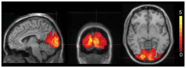
Increase in CBV (mL blood/100 mL) in the occipital cortex with visual stimulation; composite image over all volunteers.

At rest, OBV was assumed to coincide with arterial CBV; however, CBV distribution among arterial vs. capillary/venous compartments could be different during activation. While we cannot pinpoint the exact distribution of arterial vs. capillary/venous CBV changes with activation, our knowledge of the total CBV increase and oxygenation levels can determine possible ranges for these parameters as illustrated in Figure 5. In Figure 5a, FO is the fraction of oxygenated CBV (FO = OBV/CBV, with oxygenation YO = 98%), FD is the remaining deoxygenated CBV fraction (FD = 1–FO = DBV/CBV, with oxygenation YD), and Y is the resulting oxygenation (Y = YO.FO+ YD.FD). The blue curve represents Y = 74% with Point A corresponding to the assumption of FO = 21% at rest. Activation shifts Point A to the red curve representing Y = 84%. The change in CBV determines the maximum and minimum possible FO during activation, thus the range for YD. For instance, if the CBV increase of 20% occurs entirely in OBV, Point A would move to Point D; otherwise, if the CBV increase of 20% occurs entirely in DBV, Point A would move to Point E, such that YD is limited to the range ~76–81% (dashed curves, FO ~17.5–34%). Venous oxygenation in the activated brain was previously reported as 78% during visual stimulation in healthy volunteers (65), in agreement with this range. Possible parameter ranges are also shown for CBV increases of 10% and 30%. Given the depicted resting baseline CBV distribution and oxygenation, Figure 5b shows fractions (F) and oxygenations (Y) corresponding to a 20% increase in CBV occurring entirely in the arterial, capillary, or venous compartments, as well as a more realistic mixed case considering volume changes in all compartments. In the mixed case, the 20% increase in CBV was distributed as follows: 50% arterial, 30% capillary, 20% venous (i.e., CBV increase of 1.4 mL distributed as 0.7 mL arterial+0.42 mL capillary+0.28 mL venous), corresponding to an arterial CBV increase of ~50%, capillary CBV increase of ~16%, and venous CBV increase of ~10% as observed using venous refocusing for volume estimation (28).

FIG. 5.

a: Blood oxygenation as a function of the underlying CBV distribution (OBV vs. DBV) and oxygenation (of DBV), at rest and during activation. FO: fraction of oxygenated CBV (FO = OBV/CBV, with oxygenation YO = 98%); FD: fraction of deoxygenated CBV (FD = 1–FO = DBV/CBV, with oxygenation YD); Y: oxygenation (Y = YO.FO+YD.FD). Activation shifts Point A (with FO = 21% at rest) to the activation curve. The increase in CBV determines the maximum and minimum possible FO during activation, thus the range for YD. Possible parameter ranges are shown for CBV increases of 10, 20, and 30%. For instance, if the CBV increase of 20% occurs entirely in OBV, Point A moves to Point D; otherwise, if the CBV increase of 20% occurs entirely in DBV, Point A moves to Point E, limiting YD to the range ~76–81% (dashed curves, FO ~17.5–34%). b: Fractions, F, and oxygenation levels, Y, in blood compartments at baseline, and with a 20% increase in CBV shown for: the CBV increase occurring entirely on the arterial side, the capillary side, the venous side, or a more realistic distribution over the three compartments (50% of CBV increase in arterial, 30% in capillary, and 20% in venous compartments).

Quantification assumes that blood, CSF, and tissue experience the described pulse sequence; however, flow could introduce errors due to spin populations missing pulses or experiencing extra pulses. Since inversions and saturations are non-selective, uninverted or unsaturated CSF contributions from outside the imaging volume are unlikely with slow CSF flow velocities (0–2 cm/s). Figure 2 shows the region to be traversed between pulses for such contributions. In the worst-case scenario with non-tortuous superior flow, the imaging volume could include uninverted blood for velocities exceeding ~74 cm/s, or unsaturated blood for velocities exceeding ~16 cm/s, corresponding to large (~5–10 mm diameter) and small (~1 mm diameter) arteries, respectively. Following contrast bolus injection in internal carotid arteries, blood arrives in the frontal and parietal arterial tree in ~2 s with an additional ~3 s to arrive in the capillaries and another ~2 s to arrive in the veins; arrival in the occipital lobe takes an additional ~4–5 s compared to frontal and parietal areas (74). In this more realistic scenario, uninverted or unsaturated blood contributions are unlikely for vessels of interest even with smaller coil coverage.

On the other hand, spin history contamination with extra excitation pulses is possible for blood at certain velocities at certain TRs, if the time for blood to travel between two slices, Δt, equals the difference in the TI times of these slices, Δ_TI. In the rotating order, Δ_TI is a function of TR, such that blood experiencing an extra excitation in a certain TR would need to flow at a different velocity for contamination in other TRs. Secondly, blood experiencing an extra excitation in a different slice recovers from zero toward equilibrium, always reaching the same signal level at Δt, instead of following IR behavior over multiple TI times. Figure 6 depicts worst case scenarios for contamination in slices at the edge and center of the imaging volume from adjacent slices, over multiple TI times. The slowest velocities for contamination exceed those expected in microvasculature (>1.5 cm/s), but could result from a combination of large and small vessels. Slices of interest are acquired before the contaminating slices for shorter TI times, such that no contamination can occur. When the acquisition order changes and contamination from flow occurs, signal level remains constant (blue and green curves) instead of following IR behavior over TI times (black curve). Estimates are derived by fitting to signal behavior over the TI range, but both factors cause signal behavior to differ from the biophysical model, unlikely to result in fits with R²>0.95 and contribute to results, as also supported by the lack of significant spin history contamination across ascending vs. descending acquisitions.

FIG. 6.

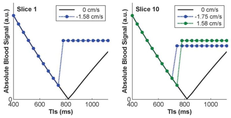
Signal with and without blood spin history contamination, shown for slices at the edge (Slice 1, left) and center (Slice 10, right) of the imaging volume over multiple TI times, with and without flow, for worst case scenarios requiring the slowest blood flow velocities. Slice 1 is most easily contaminated by superior to inferior flow of blood excited during the acquisition of Slice 2, while Slice 10 is most affected by Slices 9 or 11. No contamination can occur at shorter TI times where the slices of interest (1 and 10) are acquired before the contaminating slices (2, 9, and 11). When the acquisition order changes and contamination from flow occurs, signal level in the slices of interest remains constant (blue and green curves) instead of following IR behavior over TI times (black curve).

Absolute quantification using multiple TI values limits the current method to steady-state measurements with a minimum duration of (dynamic periods+TR × nTIs) × (2 for ON/OFF), corresponding to ~2.5 min in the current implementation. Dynamic periods between ON and OFF cycles (18 s) were allowed for settling of the hemodynamic response and unused, but could offer an opportunity for dynamic monitoring: quantitative steady-state estimates could potentially calibrate and quantify dynamic but relative CBV measurements (i.e., such as VASO which requires knowledge of resting CBV for quantification, or venous refocusing for volume estimation for venous contributions), providing a more complete picture of CBV changes during functional activation than either method alone.

CBV quantification involves more parameters than we can directly estimate from the dataset (i.e., as opposed to a simple exponential decay with two parameters), and parameters have to be assumed or separately measured. Pathologies may further limit the number of parameters that can safely be assumed. Although fast methods are available for quantification of tissue parameters (60,75), application of the current method to patients may be limited unless such parameter maps also prove valuable adjuncts to standard imaging and the remaining parameters (i.e., hematocrit, arterial oxygenation levels) can be determined in disease. CSF fraction changes with activation were negligible in the occipital cortex (50,76), and allowed us to limit the number of parameters in the current study. However, CSF may have larger effects in other brain areas (67,68,76) and it is desirable to extend the model to allow for such changes in future studies.

CONCLUSIONS

We have shown the feasibility of non-invasive absolute CBV quantification during functional activation with extended slice coverage. Our improvements enable multi-slice acquisition by rotating the slice order while maintaining balanced and consistent TI ranges across all slices, and steady-state throughout varying inversion and recovery durations. CBV estimates in healthy subjects were consistent with prior publications. The proposed method holds great potential for advancing our understanding of the fundamental physiological relationship between neural activity and hemodynamic regulation under normal, pathological, and neuronally active conditions. This approach also complements existing methods for estimating compartmental changes; and could potentially find utility in evaluating vascular health.

References

- 1.Harris GJ, Lewis RF, Satlin A, English CD, Scott TM, Yurgelun-Todd DA, Renshaw PF. Dynamic susceptibility contrast MRI of regional cerebral blood volume in Alzheimer’s disease. Am J Psychiatry. 1996;153:721–724. doi: 10.1176/ajp.153.5.721. [DOI] [PubMed] [Google Scholar]
- 2.Maas LC, Harris GJ, Satlin A, English CD, Lewis RF, Renshaw PF. Regional cerebral blood volume measured by dynamic susceptibility contrast MR. J Magn Reson Imaging. 1997;7:215–219. doi: 10.1002/jmri.1880070133. [DOI] [PubMed] [Google Scholar]
- 3.Essig M, Waschkies M, Wenz F, Debus J, Hentrich HR, Knopp MV. Assessment of brain metastases with dynamic susceptibility-weighted contrast-enhanced MR imaging: initial results. Radiology. 2003;228:193–199. doi: 10.1148/radiol.2281020298. [DOI] [PubMed] [Google Scholar]
- 4.Derdeyn CP, Videen TO, Yundt KD, Fritsch SM, Carpenter DA, Grubb RL, Powers WJ. Variability of cerebral blood volume and oxygen extraction: stages of cerebral haemodynamic impairment revisited. Brain. 2002;125 (pt 3):595–607. doi: 10.1093/brain/awf047. [DOI] [PubMed] [Google Scholar]
- 5.Kader A, Young WL. The effects of intracranial arteriovenous malformations on cerebral hemodynamics. Neurosurg Clin N Am. 1996;7:767–781. [PubMed] [Google Scholar]
- 6.Theberge J. Perfusion magnetic resonance imaging in psychiatry. Top Magn Reson Imaging. 2008;19:111–130. doi: 10.1097/RMR.0b013e3181808140. [DOI] [PubMed] [Google Scholar]
- 7.Zaharchuk G. Theoretical basis of hemodynamic MR imaging techniques to measure cerebral blood volume, cerebral blood flow, and permeability. AJNR Am J Neuroradiol. 2007;28:1850–1858. doi: 10.3174/ajnr.A0831. [DOI] [PMC free article] [PubMed] [Google Scholar]
- 8.Boxerman JL, Bandettini PA, Kwong KK, Baker JR, Davis TL, Rosen BR, Weisskoff RM. The intravascular contribution to fMRI signal change: Monte Carlo modeling and diffusion-weighted studies in vivo. Magn Reson Med. 1995;34:4–10. doi: 10.1002/mrm.1910340103. [DOI] [PubMed] [Google Scholar]
- 9.Buxton RB, Wong EC, Frank LR. Dynamics of blood flow and oxygenation changes during brain activation: the balloon model. Magn Reson Med. 1998;39:855–864. doi: 10.1002/mrm.1910390602. [DOI] [PubMed] [Google Scholar]
- 10.Ogawa S, Menon RS, Tank DW, Kim SG, Merkle H, Ellermann JM, Ugurbil K. Functional brain mapping by blood oxygenation level-dependent contrast magnetic resonance imaging. A comparison of signal characteristics with a biophysical model. Biophys J. 1993;64:803–812. doi: 10.1016/S0006-3495(93)81441-3. [DOI] [PMC free article] [PubMed] [Google Scholar]
- 11.van Zijl PC, Eleff SM, Ulatowski JA, Oja JM, Ulug AM, Traystman RJ, Kauppinen RA. Quantitative assessment of blood flow, blood volume and blood oxygenation effects in functional magnetic resonance imaging. Nat Med. 1998;4:159–167. doi: 10.1038/nm0298-159. [DOI] [PubMed] [Google Scholar]
- 12.Zhao F, Jin T, Wang P, Kim SG. Improved spatial localization of post-stimulus BOLD undershoot relative to positive BOLD. Neuroimage. 2007;34:1084–1092. doi: 10.1016/j.neuroimage.2006.10.016. [DOI] [PMC free article] [PubMed] [Google Scholar]
- 13.Lu H, Golay X, Pekar JJ, Van Zijl PC. Functional magnetic resonance imaging based on changes in vascular space occupancy. Magn Reson Med. 2003;50:263–274. doi: 10.1002/mrm.10519. [DOI] [PubMed] [Google Scholar]
- 14.Mandeville JB, Marota JJ, Kosofsky BE, Keltner JR, Weissleder R, Rosen BR, Weisskoff RM. Dynamic functional imaging of relative cerebral blood volume during rat forepaw stimulation. Magn Reson Med. 1998;39:615–624. doi: 10.1002/mrm.1910390415. [DOI] [PubMed] [Google Scholar]
- 15.Belliveau JW, Kennedy DN, Jr, McKinstry RC, Buchbinder BR, Weisskoff RM, Cohen MS, Vevea JM, Brady TJ, Rosen BR. Functional mapping of the human visual cortex by magnetic resonance imaging. Science. 1991;254:716–719. doi: 10.1126/science.1948051. [DOI] [PubMed] [Google Scholar]
- 16.Davis TL, Kwong KK, Weisskoff RM, Rosen BR. Calibrated functional MRI: mapping the dynamics of oxidative metabolism. Proc Natl Acad Sci USA. 1998;95:1834–1839. doi: 10.1073/pnas.95.4.1834. [DOI] [PMC free article] [PubMed] [Google Scholar]
- 17.Mandeville JB, Marota JJ, Ayata C, Moskowitz MA, Weisskoff RM, Rosen BR. MRI measurement of the temporal evolution of relative CMRO(2) during rat forepaw stimulation. Magn Reson Med. 1999;42:944–951. doi: 10.1002/(sici)1522-2594(199911)42:5<944::aid-mrm15>3.0.co;2-w. [DOI] [PubMed] [Google Scholar]
- 18.Hoge RD, Atkinson J, Gill B, Crelier GR, Marrett S, Pike GB. Linear coupling between cerebral blood flow and oxygen consumption in activated human cortex. Proc Natl Acad Sci USA. 1999;96:9403–9408. doi: 10.1073/pnas.96.16.9403. [DOI] [PMC free article] [PubMed] [Google Scholar]
- 19.Kastrup A, Kruger G, Glover GH, Moseley ME. Assessment of cerebral oxidative metabolism with breath holding and fMRI. Magn Reson Med. 1999;42:608–611. doi: 10.1002/(sici)1522-2594(199909)42:3<608::aid-mrm26>3.0.co;2-i. [DOI] [PubMed] [Google Scholar]
- 20.Kastrup A, Kruger G, Neumann-Haefelin T, Glover GH, Moseley ME. Changes of cerebral blood flow, oxygenation, and oxidative metabolism during graded motor activation. Neuroimage. 2002;15:74–82. doi: 10.1006/nimg.2001.0916. [DOI] [PubMed] [Google Scholar]
- 21.Kim SG, Ugurbil K. Comparison of blood oxygenation and cerebral blood flow effects in fMRI: estimation of relative oxygen consumption change. Magn Reson Med. 1997;38:59–65. doi: 10.1002/mrm.1910380110. [DOI] [PubMed] [Google Scholar]
- 22.Kim SG, Tsekos NV, Ashe J. Multi-slice perfusion-based functional MRI using the FAIR technique: comparison of CBF and BOLD effects. NMR Biomed. 1997;10:191–196. doi: 10.1002/(sici)1099-1492(199706/08)10:4/5<191::aid-nbm460>3.0.co;2-r. [DOI] [PubMed] [Google Scholar]
- 23.Grubb RL, Jr, Raichle ME, Eichling JO, Ter-Pogossian MM. The effects of changes in PaCO2 on cerebral blood volume, blood flow, and vascular mean transit time. Stroke. 1974;5:630–639. doi: 10.1161/01.str.5.5.630. [DOI] [PubMed] [Google Scholar]
- 24.Hyder F, Kida I, Behar KL, Kennan RP, Maciejewski PK, Rothman DL. Quantitative functional imaging of the brain: towards mapping neuronal activity by BOLD fMRI. NMR Biomed. 2001;14:413–431. doi: 10.1002/nbm.733. [DOI] [PubMed] [Google Scholar]
- 25.Ito H, Takahashi K, Hatazawa J, Kim SG, Kanno I. Changes in human regional cerebral blood flow and cerebral blood volume during visual stimulation measured by positron emission tomography. J Cereb Blood Flow Metab. 2001;21:608–612. doi: 10.1097/00004647-200105000-00015. [DOI] [PubMed] [Google Scholar]
- 26.Jones M, Berwick J, Mayhew J. Changes in blood flow, oxygenation, and volume following extended stimulation of rodent barrel cortex. Neuroimage. 2002;15:474–487. doi: 10.1006/nimg.2001.1000. [DOI] [PubMed] [Google Scholar]
- 27.Wu G, Luo F, Li Z, Zhao X, Li SJ. Transient relationships among BOLD, CBV, and CBF changes in rat brain as detected by functional MRI. Magn Reson Med. 2002;48:987–993. doi: 10.1002/mrm.10317. [DOI] [PubMed] [Google Scholar]
- 28.Chen JJ, Pike GB. BOLD-specific cerebral blood volume and blood flow changes during neuronal activation in humans. NMR Biomed. 2009;22:1054–1062. doi: 10.1002/nbm.1411. [DOI] [PubMed] [Google Scholar]
- 29.Griffeth VE, Buxton RB. A theoretical framework for estimating cerebral oxygen metabolism changes using the calibrated-BOLD method: modeling the effects of blood volume distribution, hematocrit, oxygen extraction fraction, and tissue signal properties on the BOLD signal. Neuroimage. 2011;58:198–212. doi: 10.1016/j.neuroimage.2011.05.077. [DOI] [PMC free article] [PubMed] [Google Scholar]
- 30.Hillman EM, Devor A, Bouchard MB, Dunn AK, Krauss GW, Skoch J, Bacskai BJ, Dale AM, Boas DA. Depth-resolved optical imaging and microscopy of vascular compartment dynamics during somatosensory stimulation. Neuroimage. 2007;35:89–104. doi: 10.1016/j.neuroimage.2006.11.032. [DOI] [PMC free article] [PubMed] [Google Scholar]
- 31.Lee SP, Duong TQ, Yang G, Iadecola C, Kim SG. Relative changes of cerebral arterial and venous blood volumes during increased cerebral blood flow: implications for BOLD fMRI. Magn Reson Med. 2001;45:791–800. doi: 10.1002/mrm.1107. [DOI] [PubMed] [Google Scholar]
- 32.Kim T, Hendrich KS, Masamoto K, Kim SG. Arterial versus total blood volume changes during neural activity-induced cerebral blood flow change: implication for BOLD fMRI. J Cereb Blood Flow Metab. 2007;27:1235–1247. doi: 10.1038/sj.jcbfm.9600429. [DOI] [PubMed] [Google Scholar]
- 33.Vazquez AL, Fukuda M, Tasker ML, Masamoto K, Kim SG. Changes in cerebral arterial, tissue and venous oxygenation with evoked neural stimulation: implications for hemoglobin-based functional neuroimaging. J Cereb Blood Flow Metab. 2010;30:428–439. doi: 10.1038/jcbfm.2009.213. [DOI] [PMC free article] [PubMed] [Google Scholar]
- 34.Stefanovic B, Hutchinson E, Yakovleva V, Schram V, Russell JT, Belluscio L, Koretsky AP, Silva AC. Functional reactivity of cerebral capillaries. J Cereb Blood Flow Metab. 2008;28:961–972. doi: 10.1038/sj.jcbfm.9600590. [DOI] [PMC free article] [PubMed] [Google Scholar]
- 35.Tian P, Teng IC, May LD, et al. Cortical depth-specific microvascular dilation underlies laminar differences in. Proc Natl Acad Sci USA. 2010;107:15246–15251. doi: 10.1073/pnas.1006735107. [DOI] [PMC free article] [PubMed] [Google Scholar]
- 36.Krieger SN, Streicher MN, Trampel R, Turner R. Cerebral blood volume changes during brain activation. J Cereb Blood Flow Metab. 2012;32:1618–1631. doi: 10.1038/jcbfm.2012.63. [DOI] [PMC free article] [PubMed] [Google Scholar]
- 37.Hua J, Qin Q, Donahue MJ, Zhou J, Pekar JJ, van Zijl PC. Inflow-based vascular-space-occupancy (iVASO) MRI. Magn Reson Med. 2011;66:40–56. doi: 10.1002/mrm.22775. [DOI] [PMC free article] [PubMed] [Google Scholar]
- 38.Hua J, Qin Q, Pekar JJ, van Zijl PC. Measurement of absolute arterial cerebral blood volume in human brain without using a contrast agent. NMR Biomed. 2011;24:1313–1325. doi: 10.1002/nbm.1693. [DOI] [PMC free article] [PubMed] [Google Scholar]
- 39.Donahue MJ, Sideso E, MacIntosh BJ, Kennedy J, Handa A, Jezzard P. Absolute arterial cerebral blood volume quantification using inflow vascular-space-occupancy with dynamic subtraction magnetic resonance imaging. J Cereb Blood Flow Metab. 2010;30:1329–1342. doi: 10.1038/jcbfm.2010.16. [DOI] [PMC free article] [PubMed] [Google Scholar]
- 40.Stefanovic B, Pike GB. Venous refocusing for volume estimation: VERVE functional magnetic resonance imaging. Magn Reson Med. 2005;53:339–347. doi: 10.1002/mrm.20352. [DOI] [PubMed] [Google Scholar]
- 41.Gu H, Lu H, Ye FQ, Stein EA, Yang Y. Noninvasive quantification of cerebral blood volume in humans during functional activation. Neuroimage. 2006;30:377–387. doi: 10.1016/j.neuroimage.2005.09.057. [DOI] [PubMed] [Google Scholar]
- 42.Glielmi CB, Schuchard RA, Hu XP. Estimating cerebral blood volume with expanded vascular space occupancy slice coverage. Magn Reson Med. 2009;61:1193–1200. doi: 10.1002/mrm.21979. [DOI] [PMC free article] [PubMed] [Google Scholar]
- 43.Lu H, van Zijl PC, Hendrikse J, Golay X. Multiple acquisitions with global inversion cycling (MAGIC): a multislice technique for vascular- space-occupancy dependent fMRI. Magn Reson Med. 2004;51:9–15. doi: 10.1002/mrm.10659. [DOI] [PubMed] [Google Scholar]
- 44.Yablonskiy DA, Haacke EM. Theory of NMR signal behavior in magnetically inhomogeneous tissues: the static dephasing regime. Magn Reson Med. 1994;32:749–763. doi: 10.1002/mrm.1910320610. [DOI] [PubMed] [Google Scholar]
- 45.Yablonskiy DA. Quantitation of intrinsic magnetic susceptibility-related effects in a tissue. Magn Reson Med. 1998;39:417–428. doi: 10.1002/mrm.1910390312. [DOI] [PubMed] [Google Scholar]
- 46.He X, Yablonskiy DA. Quantitative BOLD: mapping of human cerebral deoxygenated blood volume and oxygen. Magn Reson Med. 2007;57:115–126. doi: 10.1002/mrm.21108. [DOI] [PMC free article] [PubMed] [Google Scholar]
- 47.Lu H, van Zijl PC. Experimental measurement of extravascular parenchymal BOLD effects and tissue oxygen extraction fractions using multi-echo VASO fMRI at 1.5 and 3. 0 T. Magn Reson Med. 2005;53:808–816. doi: 10.1002/mrm.20379. [DOI] [PubMed] [Google Scholar]
- 48.Lu H, Clingman C, Golay X, van Zijl PC. Determining the longitudinal relaxation time (T1) of blood at 3. 0 Tesla. Magn Reson Med. 2004;52:679–682. doi: 10.1002/mrm.20178. [DOI] [PubMed] [Google Scholar]
- 49.Silvennoinen MJ, Clingman CS, Golay X, Kauppinen RA, van Zijl PC. Comparison of the dependence of blood R2 and R2* on oxygen saturation at 1.5 and 4. 7 Tesla. Magn Reson Med. 2003;49:47–60. doi: 10.1002/mrm.10355. [DOI] [PubMed] [Google Scholar]
- 50.Donahue MJ, Lu H, Jones CK, Edden RA, Pekar JJ, van Zijl PC. Theoretical and experimental investigation of the VASO contrast mechanism. Magn Reson Med. 2006;56:1261–1273. doi: 10.1002/mrm.21072. [DOI] [PubMed] [Google Scholar]
- 51.Donahue MJ, Hua J, Pekar JJ, van Zijl PC. Effect of inflow of fresh blood on vascular-space-occupancy (VASO) contrast. Magn Reson Med. 2009;61:473–480. doi: 10.1002/mrm.21804. [DOI] [PMC free article] [PubMed] [Google Scholar]
- 52.Zhao JM, Clingman CS, Narvainen MJ, Kauppinen RA, van Zijl PC. Oxygenation and hematocrit dependence of transverse relaxation rates of blood at 3T. Magn Reson Med. 2007;58:592–597. doi: 10.1002/mrm.21342. [DOI] [PubMed] [Google Scholar]
- 53.Spees WM, Yablonskiy DA, Oswood MC, Ackerman JJ. Water proton MR properties of human blood at 1. 5 Tesla: magnetic susceptibility. Magn Reson Med. 2001;45:533–542. doi: 10.1002/mrm.1072. [DOI] [PubMed] [Google Scholar]
- 54.Luh WM, Wong EC, Bandettini PA, Hyde JS. QUIPSS II with thin-slice TI1 periodic saturation: a method for improving accuracy of quantitative perfusion imaging using pulsed arterial spin labeling. Magn Reson Med. 1999;41:1246–1254. doi: 10.1002/(sici)1522-2594(199906)41:6<1246::aid-mrm22>3.0.co;2-n. [DOI] [PubMed] [Google Scholar]
- 55.Wong EC, Buxton RB, Frank LR. Implementation of quantitative perfusion imaging techniques for functional brain mapping using pulsed arterial spin labeling. NMR Biomed. 1997;10:237–249. doi: 10.1002/(sici)1099-1492(199706/08)10:4/5<237::aid-nbm475>3.0.co;2-x. [DOI] [PubMed] [Google Scholar]
- 56.Aguirre GK, Detre JA, Zarahn E, Alsop DC. Experimental design and the relative sensitivity of BOLD and perfusion fMRI. Neuroimage. 2002;15:488–500. doi: 10.1006/nimg.2001.0990. [DOI] [PubMed] [Google Scholar]
- 57.Wang J, Aguirre GK, Kimberg DY, Roc AC, Li L, Detre JA. Arterial spin labeling perfusion fMRI with very low task frequency. Magn Reson Med. 2003;49:796–802. doi: 10.1002/mrm.10437. [DOI] [PubMed] [Google Scholar]
- 58.Lu H, Law M, Johnson G, Ge Y, van Zijl PC, Helpern JA. Novel approach to the measurement of absolute cerebral blood volume using vascular-space-occupancy magnetic resonance imaging. Magn Reson Med. 2005;54:1403–1411. doi: 10.1002/mrm.20705. [DOI] [PubMed] [Google Scholar]
- 59.Lu H, Nagae-Poetscher LM, Golay X, Lin D, Pomper M, van Zijl PC. Routine clinical brain MRI sequences for use at 3. 0 Tesla. J Magn Reson Imaging. 2005;22:13–22. doi: 10.1002/jmri.20356. [DOI] [PubMed] [Google Scholar]
- 60.Clare S, Jezzard P. Rapid T(1) mapping using multislice echo planar imaging. Magn Reson Med. 2001;45:630–634. doi: 10.1002/mrm.1085. [DOI] [PubMed] [Google Scholar]
- 61.Wansapura JP, Holland SK, Dunn RS, Ball WS., Jr NMR relaxation times in the human brain at 3. 0 tesla. J Magn Reson Imaging. 1999;9:531–538. doi: 10.1002/(sici)1522-2586(199904)9:4<531::aid-jmri4>3.0.co;2-l. [DOI] [PubMed] [Google Scholar]
- 62.Gahan PB. Circulatory systems. In: Purves WK, Sadava D, Orians GH, Heller HC, editors. Life: the science of biology. 7. Gordonsville, VA: W.H. Freeman & Co; 2004. p. 1121. [Google Scholar]
- 63.Sharan M, Jones MD, Jr, Koehler RC, Traystman RJ, Popel AS. A compartmental model for oxygen transport in brain microcirculation. Ann Biomed Eng. 1989;17:13–38. doi: 10.1007/BF02364271. [DOI] [PubMed] [Google Scholar]
- 64.Lu H, Golay X, van Zijl PC. Intervoxel heterogeneity of event-related functional magnetic resonance imaging responses as a function of T(1) weighting. Neuroimage. 2002;17:943–955. [PubMed] [Google Scholar]
- 65.Oja JM, Gillen JS, Kauppinen RA, Kraut M, van Zijl PC. Determination of oxygen extraction ratios by magnetic resonance imaging. J Cereb Blood Flow Metab. 1999;19:1289–1295. doi: 10.1097/00004647-199912000-00001. [DOI] [PubMed] [Google Scholar]
- 66.Lacadie C, Fulbright R, Arora J, Constable R, Papademetris X. Brodmann Areas defined in MNI space using a new Tracing Tool in BioImage Suite. Proceedings of the 14th Annual Meeting of the Organization for Human Brain Mapping; Melbourne, Australia. 2008. p. 771. [Google Scholar]
- 67.Herscovitch P, Raichle ME. What is the correct value for the brain–blood partition coefficient for water? J Cereb Blood Flow Metab. 1985;5:65–69. doi: 10.1038/jcbfm.1985.9. [DOI] [PubMed] [Google Scholar]
- 68.Schutz SL. Oxygen saturation monitoring by pulse oximetry. In: Lynn-McHale DJ, Carlson KK, editors. AACN procedure manual for critical care. 4. St. Louis, MO: Elsevier Saunders; 2001. p. 77. [Google Scholar]
- 69.Grandin CB, Bol A, Smith AM, Michel C, Cosnard G. Absolute CBF and CBV measurements by MRI bolus tracking before and after acetazolamide challenge: repeatabilily and comparison with PET in humans. NeuroImage. 2005;26:525–535. doi: 10.1016/j.neuroimage.2005.02.028. [DOI] [PubMed] [Google Scholar]
- 70.Li TQ, Haefelin TN, Chan B, Kastrup A, Jonsson T, Glover GH, Moseley ME. Assessment of hemodynamic response during focal neural activity in human using bolus tracking, arterial spin labeling and BOLD techniques. Neuroimage. 2000;12:442–451. doi: 10.1006/nimg.2000.0634. [DOI] [PubMed] [Google Scholar]
- 71.Francis ST, Pears JA, Butterworth S, Bowtell RW, Gowland PA. Measuring the change in CBV upon cortical activation with high temporal resolution using look-locker EPI and Gd-DTPA. Magn Reson Med. 2003;50:483–492. doi: 10.1002/mrm.10547. [DOI] [PubMed] [Google Scholar]
- 72.Nolte J, Sundsten JW. The human brain: an introduction to its functional anatomy. St. Louis, MO: Mosby; 2002. p. xiii.p. 650. [Google Scholar]
- 73.Wu B, Li W, Avram AV, Gho SM, Liu C. Fast and tissue-optimized mapping of magnetic susceptibility and T2* with multi-echo and multi-shot spirals. Neuroimage. 2012;59:297–305. doi: 10.1016/j.neuroimage.2011.07.019. [DOI] [PMC free article] [PubMed] [Google Scholar]
- 74.Scouten A, Constable RT. VASO-based calculations of CBV change: accounting for the dynamic CSF volume. Magn Reson Med. 2008;59:308–315. doi: 10.1002/mrm.21427. [DOI] [PMC free article] [PubMed] [Google Scholar]
- 75.Scouten A, Papademetris X, Constable RT. Spatial resolution, signal-to-noise ratio, and smoothing in multi-subject functional MRI studies. Neuroimage. 2006;30:787–793. doi: 10.1016/j.neuroimage.2005.10.022. [DOI] [PubMed] [Google Scholar]
- 76.Scouten A, Constable RT. Applications and limitations of whole-brain MAGIC VASO functional imaging. Magn Reson Med. 2007;58:306–315. doi: 10.1002/mrm.21273. [DOI] [PMC free article] [PubMed] [Google Scholar]