POPULATION ATTRIBUTABLE FRACTION AS A MEASURE OF HERITABILITY IN DICHOTOMOUS TWIN DATA

Abstract

In many genetic analyses of dichotomous twin data odds ratios have been used to test hypotheses on heritability and shared common environment effects of a given disease (Lichtenstein et. al., 2000, Ahlbom et. al., 1997, Ramakrishnan, et. al., 1992, 1996). However, estimates of these two effects have not been dealt with in the literature. In epidemiology, the attributable fraction (AF), a function of the odds ratio and the prevalence of the risk factor has been used to describe the contribution of a risk factor to a disease in a given population (Leviton, 1973). In this article, we adapt the AF to quantify the heritability and the shared common environment. Twin data on cancer, gallstone disease and phobia are used to illustrate the applicability of the AF estimate as a measure of heritability.

1. INTRODUCTION

Methods for analyzing dichotomous twin data using odds ratios (or logistic regression) have been considered extensively in the literature (Ramakrishnan, et.al., 1992, 1996, Betensky et. al, 2001, Olson et al., 1996, Ananth and Preisser, 1999). These methods are primarily for testing hypotheses regarding heritability and shared common environment effects of a disease using the difference between the magnitude of the association among monozygotic (MZ) twins and the dizygotic (DZ) twins. The method suggested for analyzing dichotomous twin data (Ramakrishnan, et. al.) begins by designating one member of each twin pair as the “index” twin and the other as the “co-twin.” Then a logistic regression model of the form,

$$Y={\beta }_0+{\beta }_{1}X+{\beta }_{2}Z+{\beta }_{3}XZ,$$ (1)

where Y is the logit of the probability that the index twin has the disease, X is the indicator of co-twins disease status (1 if present and 0 if absent), Z is the indicator of zygosity coded as 1 if the pair is monozygotic (MZ) and 0.5 if the pair is dizigotic and XZ is the corresponding interaction. The 1 and 0.5 coding for zygosity is used so that different components of familial effects could be examined. Using this set up the effects for MZ and DZ twin could be written,

$$\begin{array}{cc}\hfill {\beta }_{MZ}=& {\beta }_1+{\beta }_3,\hfill \\ \hfill {\beta }_{DZ}=& {\beta }_1+0.5{\beta }_3.\hfill \end{array}$$ (2)

If there is a significant difference between the two types of twins (that is, β₁ > 0 and β₃ > 0) there is evidence of familial aggregation. The familial aggregation could be due to heritability or due to the shared common environment of the two twins. (Here, the term heritability is used loosely. It corresponds to the additive effect of the genes. See Eaves (1969) for a complete discussion of this.) It is known that the MZ twins share 100% of the genes, while the DZ twins share, on an average, 50% of the heritable genes. If an observed disease is purely genetic, the MZ coefficient and the DZ coefficient would be expected to exhibit this 2:1 ratio of the genetic composition. In other words, β₁ would be zero in equation (2) and β₃ would be greater than zero. Using this, tests for heritability, shared common environment effect or both heritability and shared common environment effects could be tested by testing the null hypotheses, β₁ = 0, and/or β₃ = 0. The logistic model could be extended to include known specific environmental variables and differences could be tested by including interaction terms.

One of the drawbacks of this approach is the arbitrary assignment of the outcome variable by the index twin. For large samples this does not pose a problem. For small samples, a simple way to account for this is to force the discordant events to be equal (i.e., assume exchangeability). Olson, et. al (1996) provide a rationale for this through the estimating equations approach under the Hardy-Weinberg law. Betensky et. al. (2001) propose a more rigorous approach, in which they simultaneously fit models for Y given X as well as X given Y and apply the generalized linear mixed models to account for the correlation between the two.

Although the hypothesis tests are useful in determining whether or not a disease (or trait) is heritable, a measure of the impact of this in the population is of interest. Measures translating the tests of heritability and shared common environment that have a statistical (or epidemiologic) interpretation are not presently available. One question of interest might be what is the excess incidence of the disease in the population due to heritability? A measure that has been proposed in the literature to answer such a question is the population Attributable Fraction (AF) (Levine, 1953, Leviton, 1973, Miettinen, 1974, Rothman, 1986, Greenland and Robins, 1988). A general definition of AF is it is the ratio of difference between the incidence rate of the disease in the overall population and the incidence rate of the disease in the exposed group to the incidence rate of the disease in the overall population. In other words it is the proportion of the incidence that would disappear when the incidence in the exposed group is reduced to the level in the unexposed group. There are several variations of the formula that is used for the calculation of this measure. These have been extensively discussed in the literature (Khoury, et. al.,1993, Rockhill, et. al., 1998). The maximum likelihood estimation of AF and its asymptotic properties have also been studied (Greeland and Drescher, 1993).

In this article, we propose a measure for the proportion of the disease incidence that is due to heritability in terms of the AF. We also provide confidence intervals for this measure, based on approximate (asymptotic) variance estimates. Properties of the asymptotic variance are examined by comparing it to bootstrap variance. Results from a simulation study examining the properties of the proposed estimate are also presented . To illustrate we apply the proposed measure to twin data on cancer, gallstone disease and phobia.

2. ESTIMATING AF AND ITS VARIANCE

We will use the definition of population AF in terms of a known prevalence of the risk factor in the population (p) and the odds ratio ψ (Levin, 1953), namely

$$AF=\frac{p(\psi -1)}{1+p(\psi -1)}.$$ (3)

While there are other ways of calculating the AF we chose this one for the following reason. The hypothesis test for the genetic effects has been developed using odds ratios (Ramakrishnan, 1991) and therefore a definition of AF that involves the odds ratios is naturally preferable. There are two variations of AF in terms of the odds ratios. One is presented in equation (3) and the other is given by p_c(ψ – 1)/ψ (Miettinen, 1974), where p_c is the proportion of risk factor among cases only, which is more applicable in case-control studies. In the genetic analyses of twin data, an individual's disease status is considered a risk factor for his/her twin. Therefore the prevalence of the risk factor is essentially the prevalence of the disease in the population and disease prevalence is often known for most populations. In addition, from a theoretical point of view, fixing the prevalence leads to a more elegant estimate for the asymptotic variance of the AF. For these reasons, the definition in (3) was chosen.

In the case of dichotomous twin data, the odds ratio represents the ratio of the odds of one twin having a disease compared to the odds of the co-twin having the same disease. Correspondingly, the AF estimates the excess fraction of disease one would observe among individuals in a twin pair due to the presence of the disease in his/her co-twin. The asymptotic variance of the maximum likelihood estimate (MLE) of AF (for a given prevalence, p) could be obtained using Taylor's series expansion and is given by,

$$V\left(\widehat{AF}\right)=\frac{p^2}{{[1+p(\widehat{\psi }-1)]}^4}V\left(\widehat{\psi }\right).$$ (4)

In section 1, we described the hypothesis tests for heritability and shared common environment using the logistic regression models. To estimate the corresponding odds ratios, the additive expressions expressed in terms of the log-odds ratios in equation (2), could be written:

$$\begin{array}{cc}\hfill {\psi }_{MZ}=& {\psi }_c{\psi }_a^2,\hfill \\ \hfill {\psi }_{DZ}=& {\psi }_c{\psi }_a.\hfill \end{array}$$

Here, ψ_MZ denotes the odds ratio for the MZ twins, ψ_DZ denotes the odds ratio for the DZ twins, ψ_e(= e^β₁) is the contribution of the shared common environment and ψ_a(= e^β₃) denotes the contribution of the heritability. Since MZ twins share 100% of the heritable genes while the DZ twins share 50% on average, the model for MZ twins has twice the contribution from the additive genetic effect.

Estimates of ψ_a and ψ_c could be derived as functions of the estimates of ψ_MZ and ψ_DZ. That is,

$$\begin{array}{cc}\hfill {\widehat{\psi }}_a=& {\widehat{\psi }}_{MZ}∕{\widehat{\psi }}_{DZ},\hfill \\ \hfill {\widehat{\psi }}_c=& {\widehat{\psi }}_{DZ}^2∕{\widehat{\psi }}_{MZ},\hfill \end{array}$$ (5)

where the estimate of the MZ and DZ odds ratios are ${\widehat{\psi }}_{MZ}=\left(A_1{D}_1\right)∕\left(B_1{C}_1\right)$ and ${\widehat{\psi }}_{DZ}=\left(A_2{D}_2\right)∕\left(B_2{C}_2\right)$, where A represents the number of concordant pairs with the disease, B and C represent the number of discordant pairs (for index and co-twin, respectively) and D represents the number of concordant pairs without the disease. The subscripts 1 and 2 denote the MZ and DZ cases, respectively. The corresponding asymptotic variances in terms of the variances of the log odds ratios is,

$$\begin{array}{cc}\hfill V\left({\widehat{\psi }}_a\right)=& {\psi }_a^2(V\left(\log \left({\widehat{\psi }}_{MZ}\right)\right)+V\left(\log \left({\widehat{\psi }}_{DZ}\right)\right))\hfill \\ \hfill =& {\psi }_a^2\left(\frac{1}{A_1}+\frac{1}{B_1}+\frac{1}{C_1}+\frac{1}{D_1}+\frac{1}{A_2}+\frac{1}{B_2}+\frac{1}{C_2}+\frac{1}{D_2}\right).\hfill \\ \hfill V\left({\widehat{\psi }}_c\right)=& {\psi }_a^2(V\left(\log \left({\widehat{\psi }}_{MZ}\right)\right)+4V\left(\log \left({\widehat{\psi }}_{DZ}\right)\right))\hfill \\ \hfill =& {\psi }_c^2\left(\frac{1}{A_2}+\frac{1}{B_2}+\frac{1}{C_2}+\frac{1}{D_2}+4\left(\frac{1}{A_2}+\frac{1}{B_2}+\frac{1}{C_2}+\frac{1}{D_2}\right)\right).\hfill \end{array}$$ (6)

The estimate of the variances in equation 4 could be obtained by substituting the MLE of the corresponding odds ratios.

Now, to obtain the estimates of the AF for the heritability and shared common environment, we substitute the estimates of ψ_a and ψ_c from equation 3 in equation 1. That is,

$$\begin{array}{cc}\hfill {\widehat{AF}}_a=& \frac{p({\widehat{\psi }}_a-1)}{1+p({\widehat{\psi }}_a-1)},\hfill \\ \hfill {\widehat{AF}}_c=& \frac{p({\widehat{\psi }}_c-1)}{1+p({\widehat{\psi }}_c-1)}.\hfill \end{array}$$ (7)

The respective asymptotic variances for the AF's could be similarly obtained by substituting from equations 3 and 4 in 2.

Typically the asymptotic variances of the estimates of AF are quite sensitive to the cell sizes as well as the total sample size. One could also apply the Bootstrap method to obtain the variance, especially when the cell size and/or the total sample size are small.

3. APPLICATIONS

Twin data on cancer, gallstone disease and phobia are used here to illustrate the estimation of AF and its variance. These data are from four published sources. The first is a compilation of data on cancer in twins from the Swedish, the Danish, and the Finnish twin registries (Lichtenstein et. al., 2000). The data consist of 44,788 pairs of twins of which there were 8,437 pairs of monozygotic women, 15,351 pairs of dizygotic women, 7,231 pairs of monozygotic men and 13,769 pairs of dizygotic men. The data consist of 28 different cancers in 10,803 individuals. Here we present the AF estimates for breast (women only), colorectal, and prostate cancers. The second is on gallstone disease in twins in the Swedish Twin Registry (Katsika et. al., 2005). A cohort of 29,256 same-sex twin pairs stratified by gender and age groups are considered here. The third is on phobias in twin children in the Swedish Twin Registry (Lichtenstein and Annas, 2000). Data on phobia were reported by parents. A cohort of 1,106 twin pairs whose parents responded to the questionnaire regarding these phobias was analyzed. Of the 1,106 pairs data from 649 same-sexed pairs were analyzed. Here we present the AF estimates for the combined data on all phobias. The data from these three sources along with odds ratios are presented in Table 1.

Table 1.

Twin Data on Cancer, Gallstone and Phobia

Phenotype	Number Discordant (B+C)	Number Concordant Affected (D)	Number Concordant Unaffected (A)	Odds-ratio (SE)
Cancers Breast
MZ	505	42	6684	4.40 (0.79)
DZ	1023	52	12694	2.52 (0.38)
Colorectum
Men
MZ	202	10	8225	8.06 (2.79)
DZ	393	17	14975	6.59 (1.73)
Women
MZ	214	20	6997	12.22 (3.21)
DZ	453	15	13301	3.89 (1.07)
Prostate Cancer
MZ	299	40	8098	14.49 (2.84)
DZ	584	20	14787	3.47 (0.83)
Other Diseases
Gallstone
Ages: 64-102
Men
MZ	280	24	2498	3.06 (0.61)
DZ	456	25	4096	1.97 (0.44)
Women
MZ	410	49	3013	3.51 (0.61)
DZ	735	63	5529	2.58 (0.38)
Ages: 44-63
Men
MZ	58	7	2116	17.61 (8.11)
DZ	124	8	3403	7.08 (2.81)
Women
MZ	208	32	2378	7.04 (1.59)
DZ	305	25	3414	3.67 (0.85)
Phobia (any)
MZ	20	11	370	40.7 (22.05)
DZ	18	3	227	8.41 (6.29)

To demonstrate the computations of the AF estimates, we will use the data on breast cancer. First we compute the odds ratios by zygosity.

The MZ odds ratio for breast cancer is:

$${\widehat{\psi }}_{MZ}=42\times 6684∕((505∕2)\times (505∕2))=4.40,$$

with

$$\mathrm{SE}\left({\widehat{\psi }}_{MZ}\right)=\sqrt{{4.40}^2\left(\frac{1}{6684}+\frac{4}{505}+\frac{1}{42}\right)}=0.79.$$

The DZ odds ratio for breast cancer is:

$${\widehat{\psi }}_{DZ}=52\times 12694∕((1023∕2)\times (1023∕2))=2.52,$$

with

$$\mathrm{SE}\left({\widehat{\psi }}_{DZ}\right)=\sqrt{{2.52}^2\left(\frac{1}{12694}+\frac{4}{1023}+\frac{1}{52}\right)}=0.38$$

Next we compute the two components of the odds ratios as shown in equation 3. The heritability component is, ${\widehat{\psi }}_a=4.40∕2.52=1.75$ with SE = 0.41 (using square root of equation 4). The common environment component is, ${\widehat{\psi }}_c=(2.52\times 2.52)∕4.40=1.45$ with SE = 0.51.

Next, to compute the AF estimates we need the prevalence of breast cancer. The prevalence of breast cancer (i.e., the proportion of women who ever were diagnosed with breast cancer) in various populations is available. In actual applications one should use the known prevalence of the disease, specific to the population being studied. Here, for illustration purposes, we calculated the prevalence as follows and assumed it to be fixed. Referring to the different numbers of pairs in table 1 we could compute the total number of breast cancers observed as, 2 × 42 + 505 + 2 × 52 + 1,023 = 1,716. The total number of women in the cohort is 42,000. Therefore, the prevalence is 1,716/42,000 = 0.041. Substituting these in equation 5, the corresponding AF's are computed as follows: The AF for heritability of breast cancer is:

$${\widehat{AF}}_a=\frac{0.041(1.75-1)}{1+0.041(1.75-1)}=0.030\text{with SE (using square root of equation 2)},0.016.$$

The AF for common environment of breast cancer is:

$${\widehat{AF}}_c=\frac{0.041(1.45-1)}{1+0.041(1.45-1)}=0.018\text{with}\mathrm{SE},0.020.$$

From these we could conclude, 3.0% (±1.6%) of the breast cancers in women is attributable to inheritance, while about 1.8% (±2.0%) of the breast cancers in women are attributable to shared common environment. In applications, since the AF estimates of the heritability and the shared common environment are correlated, if these s.e.'s are used to compute confidence intervals one should consider adjustments to the confidence levels (e.g. Bonferroni adjustment).

Since the index twin co-twin definition is arbitrary, the discordant cell probabilities are exchangeable and therefore one could consolidate the B and C cells by substituting (B + C)/2 for B and C. (This is also analogous to using a Generalized Estimating Equation logistic regression model in which the measurements from the twins are treated as repeated.) In table 1, the odds ratios and the standard errors were computed using the average of the discordant cells, by substituting (B + C)/2 for B and C cells.

In table 2 the AF for the heritability and the shared common environment along with the standard errors (SE) are presented (in percentages). For some diseases the AF estimates of the common environment effects were zero (or negative), and they corresponded to situations where they were not statistically significant. In table 2, these situations are represented by zero.

Table 2.

AF Estimates for Heritability and Common Environment

	Attributable Fraction (SE)
Phenotype	Additive Heritability	Common Environment
Breast	3.0 (1.6)	1.7 (2.0)
Colorectum
Men	0.3 (0.7)	5.6 (4.0)
Women	3.6 (1.9)	0.4 (1.3)
Prostate	6.3 (2.4)	0.0
Gallstone
Ages: 64-102
Men	3.0 (2.7)	5.8 (4.0)
Women	2.5 (2.1)	4.3 (4.4)
Ages: 44-63
Men	2.7 (2.7)	1.5 (3.5)
Women	4.3 (2.8)	3.3 (4.5)
Phobia (Any)	1.6 (1.6)	3.6 (1.3)

One of the limitations of most analyses of twin studies is that the standard errors are large even when the total sample sizes are in the thousands. This is the case in our applications as well. A Bootstrap approach was also applied to estimate the variances in order to examine if the asymptotic approximation of the variances were adequate. For each of the phenotype, one thousand Bootstrap samples with replacement were drawn. So, for example, in the case of breast cancer, random samples with replacement from the 7,231 pairs of observations were drawn and the corresponding frequencies (as shown in table 1) were obtained. For each of these data, keeping the prevalence constant, (e.g. fixed at 4.1% for the breast cancer), the two AF's were estimated. The Bootstrap variance was obtained from the distribution of these estimates. These Bootstrap variances are presented in Table 3. The differences observed in the two methods seem negligible and therefore one might conclude that the asymptotic approximation is reasonable.

Table 3.

Bootstrap Estimates for the Variance of AF

	Actual Data		Bootstrap Estimates		Actual Data		Bootstrap Estimates
	AFa	Asymptotic Variance of AFa	AFa	Variance of AFa	AFc	Asymptotic Variance of AFc	AFc	Variance of AFc
Breast Cancer	0.03	0.000248	0.03	0.000242	0.02	0.000405	0.02	0.000430
Colorectal Cancer
Male	0.00	0.000052	0.00	0.000071	0.06	0.001694	0.07	0.002768
Female	0.04	0.000379	0.04	0.000531	0.00	0.000172	0.01	0.000247
Prostate Cancer	0.06	0.000570	0.07	0.000654	0.00	0.000082	0.00	0.000094
Gallstone
Male – 64-102 years	0.03	0.000717	0.03	0.000804	0.01	0.001221	0.02	0.001531
Female – 64-102 years	0.02	0.000426	0.03	0.000434	0.06	0.001599	0.06	0.001643
Gallstone
Male – 44-63 years	0.03	0.000706	0.04	0.001676	0.03	0.002054	0.05	0.004960
Female – 44-63 years	0.04	0.000780	0.05	0.000956	0.04	0.001974	0.05	0.002240
Phobia (any)	0.16	0.025336	0.22	0.035641	0.04	0.017054	0.11	0.036453

4. SIMULATING TWIN DATA

In this section, first we introduce a method for simulating twin data given values of AF for heritability, AF for shared common environment and prevalence of a disease. Then using this method a simulation study is performed to examine the properties of the estimates of AF. Specifically, the purpose of the simulation study is to examine how the bias and the mean square error (MSE) of the estimates change as a function of the prevalence of the phenotype and the size of the sample.

Consider the following 2 × 2 table showing the probabilities of the disease statuses, where twins are labeled arbitrarily as twin 1 and twin 2.

Twin 1	Twin 2
	Yes	No
Yes	π1	π2
No	π2	π3

The cell probabilities are uniquely defined for a given prevalence p and AF as shown below. Using equation (1) for a specified p and AF the corresponding odds ratio for the table, Ψ, could be calculated using

$$\Psi =1-\left(\frac{AF}{p(AF-1)}\right).$$ (8)

Then the cell probabilities can be uniquely determined by solving the simultaneous equations,

$$\begin{array}{cc}\hfill \frac{{\pi }_1{\pi }_3}{{\pi }_2^2}=& \Psi ,\hfill \\ \hfill {\pi }_1+{\pi }_2=& p,\hfill \\ \hfill {\pi }_1+2{\pi }_2+{\pi }_3=& 1.\hfill \end{array}$$ (9)

Solving these equations yield,

$$\begin{array}{cc}\hfill {\pi }_2=& \left(\sqrt{1+4(\Psi -1)p(1-p)}-1\right)∕2(\Psi -1),\hfill \\ \hfill {\pi }_1=& p-{\pi }_2,\hfill \\ \hfill {\pi }_3=& 1-p-{\pi }_2.\hfill \end{array}$$ (10)

Once these cell probabilities are obtained for a given prevalence, AF_a and AF_c, generating the table for a given sample size is straight forward. A macro in SAS® IML was written to generate the data tables. The input to this macro includes the desired number of simulations, the desired sample size, and the desired cell probabilities and from this generates random multinomial samples using the RANDMULTINOMIAL function in SAS® IML. A selected number of combinations of levels of AF_a, AF_c, prevalence p and sample sizes 2 × 2 tables were generated. The levels were chosen based on the range of values observed in the applications presented in section 3. The levels considered are,

$$\begin{array}{cc}\hfill A{F}_a:& 0.03,0.15,0.30\hfill \\ \hfill A{F}_c:& 0.00,0.03,0.15\hfill \\ \hfill \text{Prevalence},p:& 0.05,0.10,0.20\hfill \end{array}$$

These lead to 64 scenarios many of which lead to unrealistic odds ratios. Therefore, 34 combinations resulting in MZ and DZ odds ratio less than 26.0 (again based on the data in the literature) were selected for the simulations. For each of the 34 combinations 1,000 simulations were performed for MZ twin sample sizes of 900, 1,800 and 3,600. (The DZ twin sample sizes were set to be equal to twice as many as MZ twins.)

For each combination, the simulations yielded estimates of the attributable fractions for the shared common environment (AF_c) and the heritable (AF_a) components. The bias and the mean squared error (MSE) were calculated for each combination. The results are presented in Figures 1 and 2. The Figure 1 plots the bias squared versus the MSE for the estimates of AF_a for a each level of AF_c (1a – 1c). Each line represents a certain prevalence and AF_a for decreasing levels of the sample size. The Figure 2 is the corresponding plot for the estimates of AF_c. All the plots show, as expected, large sample sizes lead to small biases as well as MSE's (shown by the clustering of points near the origin in all the plots). The following additional conclusions specific to other simulation conditions emerge.

1. As the prevalence increases the bias for both AF_a and AF_c decreases, irrespective of the sample size. (Figures 1a – 1c).

2. The bias for AF_a is smaller for larger magnitude of AF_a, irrespective of the magnitude of AF_c (Figures 1a – 1c). Similarly, the bias for AF_c is smaller for larger magnitude of AF_a, irrespective of the magnitude of AF_a (Figures 2a – 2c).

3. The bias of AF_a are smaller for smaller magnitudes of AF_a. However, for certain cases the decrease in the MSE is not linear (Figure 1a).

4. The larger the value of AF_c the more accurate (i.e. smaller bias and MSE) the estimates of AF_a. Similarly the larger the value of AF_a the more accurate the estimates of AF_c.

Figure 1.

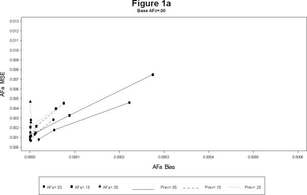
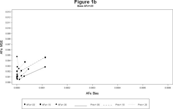
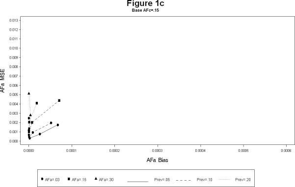
AF_a bias and MSE for simulation scenarios.

Figure 2.

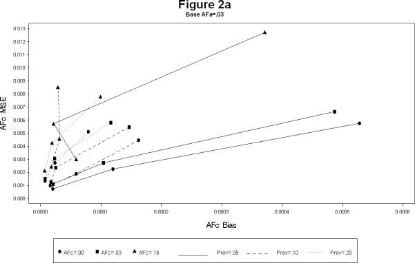
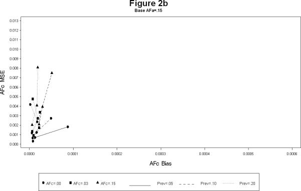
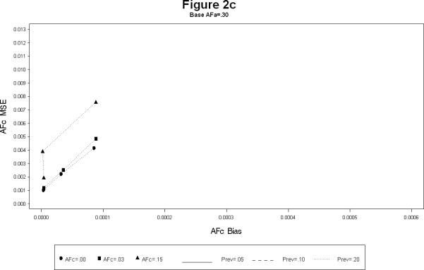
AF_a bias and MSE for simulation scenarios.

In summary, the simulation study seem to indicate that the estimation of the attributable fractions for the heritable and the common environment components is best when the sample size is over 1,800 MZ twin pairs (3,600 DZ twin pairs), The estimates are reasonable in terms of bias and MSE, if the disease prevalence is large (at least 15%), or the heritable component is of large magnitude (at least 0.15) .

5. DISCUSSION

We have provided here a measure for describing the heritability and shared common environment effects in dichotomous twin studies using the attributable fraction. We have also provided a simple method to calculate the asymptotic variance of the estimate of AF assuming the prevalence of the disease to be known. The AF is based on a combination of the odds ratio and the prevalence of the risk factor in question. Thus, it combines the magnitude of the risk associated with a risk factor and the prevalence of that risk factor. Hence, it aims at providing a measure of the public health impact of a risk factor on the disease in question. Several articles in the field of epidemiology caution the researchers regarding the use and interpretation of AF. A careful consideration of the issues discussed in these articles lead us to believe that the most appropriate use of AF might be in twin studies.

Although we have provided formulas for computing the estimate of AF and its variance using the 2 × 2 table entries of the MZ and DZ tables, the estimates of the odds ratios (or the log odds ratios) and their variances could also be obtained from a repeated measures logistic regression method (as described in section 3). (There are several programs that can provide these estimates directly. For instance, PROC GLIMMIX in SAS® or STATA could be used.). Once these estimates are available a direct substitution in the equations 2, 3 and 4 will yield the corresponding MLEs of the AFs and their asymptotic variances.

While the asymptotic variance estimates provided are appropriate, as confirmed by the bootstrap estimates, the asymptotic distribution of the estimate of AF needs to be further explored. Typically, the log of the estimate of AF better approximates normality. For this reason, to construct confidence intervals the log transformation may be considered. It is also important to point out here that the estimates of odds ratios (and consequently the estimates of AF) have large variances when cell sizes in the 2 × 2 tables are small. Therefore, the method is suitable for twin data from large registries, such as the Swedish Twin Registry, but may not be suitable for small samples.

In our illustrations, the prevalence was estimated from the data and assumed fixed. The uncertainty in the estimate of prevalence is thus ignored. In reality, when independent estimates of prevalence are not available, and are estimated from the data this uncertainty can not be ignored. In this case, once should use the asymptotic estimator of the variance of AF (Greenland, 1993).

The estimates proposed here for the AF could be extended to stratified analyses in which one may consider specific environment effects. This could be achieved by fitting the appropriate repeated measures logistic regression model (or the alternating logistic regression model) to the data and extracting the corresponding stratified estimates of the MZ and DZ odds ratios and their variances. For example, in the gallstone data one could fit a model including age groups and gender along with the zygosity and directly obtain adjusted odds ratios and there SE's. However, if there are confounding factors the formula of AF provided in equation 2 may have to be appropriately modified (13). The method also extends easily to bivariate situations, where two diseases are simultaneously considered.

LIST OF ABBREVIATIONS

MZ

Monozygotic

DZ

Dizygotic

AF

Attributable Fraction

MLE

Maximum Likelihood Estimate

SEM

Structural Equation Model

ACE

Used in SEM for twin data to represent a model with Additive genetics, Common environment and Error effects

REFERENCES

- Ahlbom A, Lichtenstein P, Malmström H, Feychting M, Hemminki K, Pedersen NL. Cancer in twins: genetic and nongenetic familial risk factors. Journal of the National Cancer Institute. 1997;89:287–93. doi: 10.1093/jnci/89.4.287. [DOI] [PubMed] [Google Scholar]
- Ananth C, Pressier J. Bivariate Logistic Regression: Modeling the Association of Small for Gestational Age Births in Twin Gestations. Statistics in Medicine. 1999;18:2011–2023. doi: 10.1002/(sici)1097-0258(19990815)18:15<2011::aid-sim169>3.0.co;2-8. [DOI] [PubMed] [Google Scholar]
- Betensky R, Hudson J, Jones C, Hu F, Wang B, Chen C, Xu X. A Computationally Simple Test of Homogeneity of Odds Ratios for Twin Data. Genetic Epidemiology. 2001;20:228–238. doi: 10.1002/1098-2272(200102)20:2<228::AID-GEPI5>3.0.CO;2-4. [DOI] [PubMed] [Google Scholar]
- Granström C, Sundquist J, Hemminki K. Population attributable risks for breast cancer in Swedish women by morphological type. Breast Cancer Research and Treatment. 2008;111:559–568. doi: 10.1007/s10549-007-9814-2. [DOI] [PubMed] [Google Scholar]
- Greenland S, Robins JM. Conceptual Problems in the Definition and Interpretation of Attributable Fractions. American Journal of Epidemiology. 1988;128:1185–1197. doi: 10.1093/oxfordjournals.aje.a115073. [DOI] [PubMed] [Google Scholar]
- Greenland S, Drescher K. Maximum Likelihood Estimation of the Attributable Fraction from Logistic Models. Biometrics. 1993;49:865–872. [PubMed] [Google Scholar]
- Katsika D, Grjibovski A, Einarsson C, Lammert F, Lichtenstein P, Marschall H. Genetic and Environmental Influences on Symptomatic Gallstone Disease: a Swedish Study of 43,141 Twin Pairs. Hepatology. 2005;41:1138–1143. doi: 10.1002/hep.20654. [DOI] [PubMed] [Google Scholar]
- Khoury MJ, Beaty TH, Cohen BH. Fundamentals of Genetic Epidemiology. Oxford University Press; New York: 1993. [Google Scholar]
- Levin ML. The Occurrence of Lung Cancer in Men. Acta Unio International Contra Cancrum. 1973;9:531–541. [PubMed] [Google Scholar]
- Leviton A. Definitions of Attributable Risk. American Journal of Epidemiology. 1973;98:231. doi: 10.1093/oxfordjournals.aje.a121552. [DOI] [PubMed] [Google Scholar]
- Lichtenstein P, Holm N, Verkasalo P, Iliadou A, Kaprio J, Koskenvuo M, Pukkala E, Skytthe A, Hemminki K. Environmental and Heritable Factors in the Causation of Cancer. New England Journal of Medicine. 2000;343:78–85. doi: 10.1056/NEJM200007133430201. [DOI] [PubMed] [Google Scholar]
- Miettinen OS. Proportion of Disease Caused or Prevented by a given Exposure Trait or Intervention. American Journal of Epidemiology. 1974;99:325–332. doi: 10.1093/oxfordjournals.aje.a121617. [DOI] [PubMed] [Google Scholar]
- Olson J, Witte J, Elston R. Association Within Twin Pairs for Dichotomous Trait. Genetic Epidemiology. 1996;13:489–499. doi: 10.1002/(SICI)1098-2272(1996)13:5<489::AID-GEPI5>3.0.CO;2-Y. [DOI] [PubMed] [Google Scholar]
- Ramakrishnan V, Goldberg J, Henderson W, Elsen S, True W, Lyons M, Tsuang M. Elementary Methods for the Analysis of Dichotomous Outcomes in Unselected Samples of Twins. Genetic Epidemiology. 1992;9:273–287. doi: 10.1002/gepi.1370090406. [DOI] [PubMed] [Google Scholar]
- Ramakrishnan V, Meyer J, Goldberg J, Henderson W. Univariate Analysis of Dichotomous or Ordinal Data from Twin Pairs: A Simulation Study Comparing Structural Equation Modeling and Logistic Regression. Genetic Epidemiology. 1996;13:79–90. doi: 10.1002/(SICI)1098-2272(1996)13:1<79::AID-GEPI7>3.0.CO;2-1. [DOI] [PubMed] [Google Scholar]
- Rockhill B, Newman B, Weinberg C. Use and Misuse of Population Attributable Fractions. American Journal of Public Health. 1998;88:15–19. doi: 10.2105/ajph.88.1.15. [DOI] [PMC free article] [PubMed] [Google Scholar]
- Rothman KJ. Modern Epidemiology. Little, Brown; Boston: 1986. [Google Scholar]