

Abstract
Images, often stored in multidimensional arrays, are fast becoming ubiquitous in medical and public health research. Analyzing populations of images is a statistical problem that raises a host of daunting challenges. The most significant challenge is the massive size of the datasets incorporating images recorded for hundreds or thousands of subjects at multiple visits. We introduce the population value decomposition (PVD), a general method for simultaneous dimensionality reduction of large populations of massive images. We show how PVD can be seamlessly incorporated into statistical modeling, leading to a new, transparent, and rapid inferential framework. Our PVD methodology was motivated by and applied to the Sleep Heart Health Study, the largest community-based cohort study of sleep containing more than 85 billion observations on thousands of subjects at two visits. This article has supplementary material online.
Keywords: Electroencephalography, Signal extraction
1. INTRODUCTION
We start by considering the following thought experiment using data displayed in Figure 1. Inspect the plot for a minute and try to remember it as closely as possible; ignore the meaning of the data and try to answer the following question: “How many features (patterns) from this plot do you remember?” Now, consider the case when you are flipping through thousands of similar images and try to answer the slightly modified question: “How many common features from all these plots do you remember?” Regardless of who is answering either question, the answer for this dataset seems to be invariably between 3 and 25.
Figure 1.
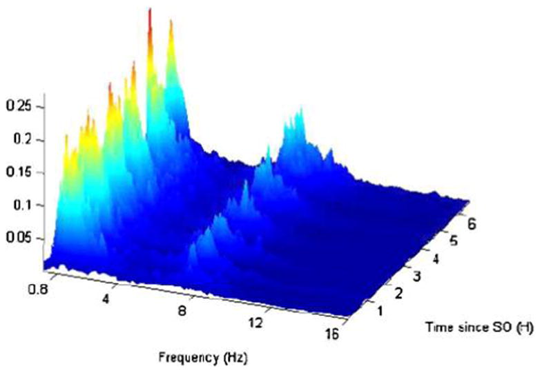
Frequency by time percent power for the sleep electroencephalography data for one subject. The Y -axis is time in hours since sleep onset, where each row corresponds to a 30-second interval. The X-axis is the frequency from 0.2 Hz to 16 Hz. The other frequencies were not shown because they are “quiet”; that is, the proportion of power in those frequencies is very small.
To mathematically represent this experiment, we introduce the population value decomposition (PVD) of a sample of matrices. In this section we focus on providing the intuition. We introduce the formal definition in Section 3. Consider a sample Yi, i = 1, …, n, of matrices of size F × T, where F, T, or both are very large. Suppose that the following approximate decomposition holds:
| (1) |
where P and D are population-specific matrices of size F × A and B × T, respectively. If A or B is much smaller than F and T, then equation (1) provides a useful representation of a sample of images. Indeed, the “subject-level” features of the image are coded in the low-dimensional matrix Vi, whereas the “population frame of reference” is coded in the matrices P and D. Important differences between PVD and the singular value decomposition (SVD) are that (a) PVD applies to a sample of images not just one image; (b) the matrices P and D are population-, not subject-, specific; and (c) the matrix Vi is not necessarily diagonal.
With this new perspective, we can revisit Figure 1 to provide a reasonable explanation for how our vision and memory might work. First, the image can be decomposed using a partition of frequencies and time in several subintervals. A checkerboard-like partition of the image is then obtained by building the two-dimensional partitions from the one-dimensional partitions. The size of the partitions is then mentally adjusted to match the observed complexity in the image. When decomposing a sample of images, the thought process is similar, except that some adjustments are made on the fly to ensure maximum encoding of information with a minimum amount of memory. Some smoothing across subjects further improves efficiency by taking advantage of observed patterns across subjects. A mathematical representation of this process would be to consider subject-specific matrices, P and D, with columns and rows corresponding to the one-dimensional partitions. The matrix Vi is then constructed by taking the average of the image in the induced two-dimensional subpartition. Our methods transfer this empirical reasoning into a statistical framework. This process is crucial for the following reasons:
Reducing massive images to a manageable set of coefficients that are comparable across subjects is of primary importance. Note that Figure 1 displays 57,000 observations, only a fraction of the total of 228,160 observations of the original uncut image. The matrix Vi typically contains fewer than 100 entries.
Statistical inference on samples of images is typically difficult. For example, the Sleep Heart Health Study (SHHS), described in Section 2, contains one image for each of two visits for more than 3000 subjects. The total number of observations used in the analysis presented in Section 5 exceeds 450,000,000. In contrast, replacing Yi by Vi reduces the dataset to 600,000 observations.
Obtaining the coefficient matrix Vi is easy once P and D are known. Using the entries of Vi as predictors in a regression context is then straightforward; this strategy was used by Caffo et al. (2010) for predicting the risk of Alzheimer’s disease using functional magnetic resonance imaging (fMRI).
Modeling of the coefficients Vi can replace modeling of the images Yi. In Section 3 we show that the Karhunen–Loève (KL) decomposition (Loève 1945; Karhunen 1947) of a sample of images can be approximated by using a computationally tractable algorithm based on the coefficients Vi. This avoids the intractable problem of calculating and diagonalizing very large covariance operators.
The article is organized as follows. In Section 2 we introduce the SHHS and the associated methodological challenges. In Section 3 we introduce the PVD and describe its application to the analysis of samples of images. Section 4 provides simulations, and Section 5 provides extensive results for the analysis of the SHHS dataset. Section 6 presents some unresolved methodological and applied problems.
2. THE CASE STUDY
The SHHS is a landmark study of sleep and its impacts on health outcomes. A detailed description of the SHHS has been provided by Quan et al. (1997), Crainiceanu, Staicu, and Di (2009), and Di et al. (2009). The SHHS is a multicenter cohort study that used the resources of existing epidemiologic cohorts and conducted further data collection, including measurements of sleep and breathing. Between 1995 and 1997, in-home polysomnography (PSG) data were collected from a sample of 6441 participants. A PSG is a quasi-continuous multichannel recording of physiological signals acquired during sleep that include two surface electroencephalograms (EEG). After the baseline visit, a second SHHS follow-up visit was undertaken between 1999 and 2003 that included a repeat PSG. A total of 4361 participants completed a repeat in-home PSG. The main goals of the SHHS were to quantify the natural variability of complex measurements of sleep in a large community cohort, to identify potential biomarkers of cardiovascular and respiratory disease, and to study the association between these biomarkers and various health outcomes, including sleep apnea, cardiovascular disease, and mortality.
Our focus on sleep EEG is based on the expectation that a spectral analysis of electroneural data will provide a set of reliable, reproducible, and easily calculated biomarkers. Currently, quantification of sleep in most research settings is based on a visual-based counting process that attempts to identify brief fluctuations in the EEG (i.e., arousals) and classify time-varying electrical phenomena into discrete sleep stages. Although metrics of sleep based on visual scoring have been shown to have clinically meaningful associations, they are subject to several limitations. First, interpretation of scoring criteria and lack of experience can increase error variance in the derived measures of sleep. For example, even with the most rigorous training and certification requirements, technicians in the large multicenter SHHS were noted to have an intraclass correlation coefficient of 0.54 for scoring arousals (Whitney et al. 1998). Second, there is a paucity of definitions for classifying EEG patterns in disease states, given that the criteria were developed primarily for normal sleep. Third, many of the criteria do not have a biological basis. For example, an amplitude criterion of 75 μV is used for the identification of slow waves (Redline et al. 1998), and a shift in EEG frequency for at least 3 seconds is required for identifying an arousal. Neither of these criteria is evidence-based. Fourth, visually scored data are described with summary statistics of different sleep stages, resulting in complete loss of temporal information. Finally, visual assessment of overt changes in the EEG provides a limited view of sleep neurobiology. In the setting of sleep-disordered breathing, a disorder characterized by repetitive arousals, visual characterization of sleep structure cannot capture common EEG transients. Thus it is not surprising that previous studies have found weak correlations between conventional sleep stage distributions, arousal frequency, and clinical symptoms (Guilleminault et al. 1988; Cheshire et al. 1992; Martin et al. 1997; Kingshott et al. 1998). Power spectral analysis provides an alternate and automatic means for the studying of the dynamics of the sleep EEG, often demonstrating global trends in EEG power density during the night. Although quantitative analysis of EEG has been used in sleep medicine, its use has focused on characterizing EEG activity during sleep in disease states or in experimental conditions. A limited number of studies have undertaken analyses of the EEG throughout the entire night to delineate the role of disturbed sleep structure in cognitive performance and daytime alertness. However, most of these studies are based on samples of fewer than 50 subjects and thus are not generalizable to the general population. Finally, there are only isolated reports using quantitative techniques to characterize EEG during sleep as a function of age and sex, with the largest study consisting of only 100 subjects.
To address these problems, here we focus on the statistical modeling of the time-varying spectral representation of the subject-specific raw EEG signal. The main components of this strategy are as follows:
-
C1
RAW SIGNAL ↦ IMAGE (FFT).
-
C2
FREQUENCY × TIME IMAGE ↦ IMAGE CHARACTERISTICS (PVD).
-
C3
ANALYZE IMAGE CHARACTERISTICS (FPCA and MFPCA).
Component C1 is a well-established data transformation and compression technique at the subject level. Even though we make no methodological contributions in C1, its presentation is necessary to understand the application. The technical details of C1 are provided in Sections 2.1 and 2.2. Component C2, our main contribution, is a second level of compression at the population level. This is an essential component when images are massive, but could be eliminated when images are small. Methods for C2 are presented in Section 3. Component C3, our second contribution, generalizes multilevel functional principal component analysis (MFPCA) (Di et al. 2009) to multilevel samples of images. Technical details for C3 are presented in Sections 3.2.1 and 3.2.2.
2.1 Fourier Transformations and Local Spectra
In the SHHS, EEG sampled at a frequency of 125 Hz (125 observations per second) and an 8-hour sleep interval will contain U = 125 Hz × 60″ × 60′ × 8h = 3,600,000 observations. A standard data-reduction step for EEG is to partition the entire time series into adjacent 5-second intervals. The 5-second intervals are further aggregated into adjacent groups of six intervals for a total time of 30 seconds. These adjacent 30-second intervals are called epochs. Thus, for an 8-hour sleep interval, the number of 5-second intervals is U/625 = 5760, and the number of epochs is T = U/(625 × 6) = 960. In general, U and T are subject- and visit-specific, because the duration of sleep is subject- and visit-specific.
Now consider the partitioned data and let xth(n) denote the nth observation of the raw EEG signal, n = 1, …, N = 625, in the hth 5-second interval, h = 1, …, H = 6, of the tth 30-second epoch, t = 1, …, T. In each 5-second window, data are first centered around their mean. We continue to denote the centered data by xth(n). We then apply a Hann weighting window to the data, which replaces the xth(n) with w(n)xth(n), where w(n) = 0.5 – 0.5 cos{2πn/(N − 1)}. To these data we apply a Fourier transform and obtain for k = 0, …, N − 1. Here Xth(k) are the Fourier coefficients corresponding to the hth 5-second interval of the tth epoch and frequency f = k/5. For each each frequency, f = k/5, and 30-second epoch, t, we calculate the average over the H = 6 5-second intervals of the square of the Fourier coefficients. More precisely, . Total power in a spectral window can be calculated as PSb(t) = Σf ∈Db P(f, t), where Db denotes the spectral window (collection of frequencies) indexed by b.
In this article we focus on P(f, t) and treat it as a bivariate function of frequency f (expressed in Hz) and time t (expressed in epochs). The power in a spectral window, PSb(t), was analyzed by Crainiceanu et al. (2009) and Di et al. (2009). Here we concentrate on methods that generalize the spirit of the methods of Di et al. (2009), while focusing on solutions to the much more ambitious problem of population-level analysis of images. Before describing our methods, we provide more insight into the interpretation of the frequency–time analysis.
2.2 Insight Into the Discrete Fourier Transform
First, note that the inverse Fourier transform is , and the Fourier coefficients are the projections of the data on the orthonormal basis e2πkni/N, k = 0, …, N − 1. Thus a larger (in absolute value) Xth(k) corresponds to a larger contribution of the frequency k/5 to explaining the raw signal. Parseval’s theorem provides the following equality: . The left side of the equation is the total observed variance of the raw signal, and the right side provides an ANOVA-like decomposition of the variance as a sum of |Xth(k)|2. This is the reason why |Xth(k)|2 is interpreted as the part of variability explained by frequency f = k/5. In signal processing |Xth(k)|2 is called the power of the signal in frequency f = k/5.
We complete our preprocessing of the data by normalizing the observed power as Y(f, t) = P(f, t)/Σf P(f, t), which is the “proportion” of observed variability of the EEG signal attributable to frequency f in epoch t. In practice, for surface EEG, frequencies above 32 Hz make a negligible contribution to the total power, and we define Y(f, t) = P(f, t)/Σf≤32 P(f, t). We call Y(f, t) the normalized power, and the true signal measured by Y(f, t) the frequency-by-time image of the EEG time series.
Figure 1 shows a frequency-by-time plot of Y(f, t) for one subject who slept for more than 6 hours. The X-axis is the frequency from 0.2 Hz to 16 Hz. The other frequencies were not shown because they are “quiet”; that is, the proportion of power in those frequencies is very small. The Y-axis is time in hours since sleep onset, with each row corresponding to a 30-second interval. Note that a large proportion of the observed variability is in the low-frequency range, say [0.8–4.0 Hz]. This range, known as the δ-power band, is traditionally analyzed in sleep research by averaging the frequency values across all frequencies in the range. Another interesting range of frequencies is roughly between 5 and 10 Hz, with the proportion of power quickly converging to 0 beyond 12–14 Hz. The [5.0–10.0 Hz] range is not standard in EEG research. Instead, research tends to focus on the θ [4.1–8.0 Hz] and α [8.1–13.0 Hz] bands. A careful inspection of the plot will reveal that in the δ, θ, and α frequency ranges the proportion of power tends to show cycles across time. (Note the wavy pattern of the data as time progresses from sleep onset.) Although this may be less clear from Figure 1, the behavior of the δ band tends to be negatively correlated with θ and α bands. This occurs because there is a natural trade-off between slow and fast neuronal firing.
3. POPULATION VALUE DECOMPOSITION
In this section we introduce a population-level data compression that allows the coefficients of each image to be comparable and interpretable across images. If Yi, i = 1, …, n, is a sample of F × T-dimensional images, then a PVD is
| (2) |
where P and D are population-specific matrices of size F × A and B × T, Vi is an A × B-dimensional matrix of subject-specific coefficients, and Ei is an F × T -dimensional matrix of residuals. Many different decompositions of type (2) exist. Consider, for example, any two full-rank matrices P and D, where A < F and B < T. Equation (2) can be written in vector format as follows. Denote by , εi = vec(eT) the column vectors obtained by stacking the row vectors of Yi, Vi, and Ei, respectively. If X = P ⊗ DT is the FT × AB Kronecker product of matrices P and D, then equation (2) becomes the following standard regression: yi = Xvi + εi. Thus a least squares estimator of vi is v̂i = (X′X)−1X′yi. This provides a simple recipe for obtaining the subject-specific scores, vi or, equivalently, Vi, once the matrices P and D are fixed. The scores can be used in standard statistical models either for prediction or for association studies. Note that X′X is a low-dimensional matrix that is easily inverted. Moreover, all calculations can be done on even very large images by partitioning files into subfiles and using block-matrix computations.
3.1 Default Population Value Decomposition
There are many types of PVDs, and definitions can and will change in particular applications. In this section we introduce our default procedure, which is inspired by the subject-specific SVD and by the thought experiment described in Section 1. Consider the case where the SVD can be obtained for every subject-specific image. This can be done in all applications that we are aware of, including the SHHS and fMRI studies (see Caffo et al. 2010 for an example).
For each subject, let be the SVD of the image. If Ui and Vi were the same across all subjects, then the SVD would be the default PVD. However, in practice Ui and Vi will tend to vary from person to person. Mimicking the thought process described in Section 1, we try to find the common features across subjects among the column vectors of the Ui and Vi matrices.
We start by considering the F × Li-dimensional matrix ULi, consisting of the first Li columns of the matrix Ui, and the T × Ri-dimensional matrix, consisting of the first Ri columns of the matrix Vi. The choices of Li and Ri could be based on various criteria, including variance explained, signal-to-noise ratios, and practical considerations. This is not a major concern in this article.
We focus on ULi; a similar procedure is applied to VRi. Consider the F × L-dimensional matrix U = [UL1|, …, |ULn], where , obtained by horizontally binding the ULi matrices across subjects. The space spanned by the columns of U is a subspace of ℝF and contains subject-specific left eigenvectors that explain most of the observed variability. Although these vectors are not identical, they will be similar if images share common features. Thus, we propose applying PCA to the matrix UUT to obtain the main directions of variation in the column space of U. Let P be the F × A-dimensional matrix formed with the first A eigenvectors of UUT as columns, where A is chosen to ensure that a certain percentage of variability is explained. Then the matrix U is approximated via the projection equation U ≈ P(PTU). At the subject level, we obtain ULi ≈ P(PT ULi). This approximation becomes a tautological equality if A = F, that is, if we use the entire eigen-basis. Similar approximations can be obtained using any orthonormal basis; we prefer the eigenbasis for our default procedure, because it is parsimonious. We similarly obtain DT, a T × B-dimensional matrix of the first eigenvectors of the matrix VVT, where V = [VR1 |, …, |VRn]. We have the similar approximation V ≈ D(DT V). At the subject level, we obtain VRi ≈ DT (DVRi). We conclude that PVD is a two-step approximation process for all images that can be summarized as follows:
| (3) |
where ULi and VRi are obtained by retaining the first Li and Ri columns from the matrices Ui and Vi, respectively, and ΣLiRi is obtained by retaining the first Li rows and Ri columns from the matrix Σi. The first approximation of the image Yi, given in the first row in equation (3), is obtained by retaining the left and right eigenvectors that explain most of the observed variability at the subject level. The second approximation, shown in the second row in equation (3), is obtained by projecting the subject-specific left and right eigenvectors on the corresponding population-specific eigenvectors.
If we denote by , we then obtain the PVD equation (2). This formula shows that Vi generally will not be a diagonal matrix even though ΣLi,Ri is. This is one of the fundamental differences between SVD and PVD. Note that all approximations can be trivially transformed into equalities. For example, choosing Li = F and Ri = T will ensure equality in the first approximation, whereas choosing A = F and B = T will ensure equality in the second equation. From a practical perspective, these cases are not of scientific importance, because data compression would not be achieved. However, our focus is on parsimony, not on perfection of the approximation. The choices of Li, Ri, A, and B could be based on various criteria, including variance explained, signal-to-noise ratios, and practical considerations. In this article we use thresholds for the percent variance explained.
Calculations in this section are possible because of the following matrix algebra trick. We summarize this trick, which allows calculation of SVD for very large matrices as long as one of the dimensions is not much larger than a few thousands.
Suppose that Y = UDVT is the SVD decomposition of an F × T -dimensional matrix where, say, F is very large and T is moderate. Then D and V can be obtained from the spectral decomposition of the T × T -dimensional matrix YTY = VD2VT. The U matrix can then be obtained from U = YVD−1.
3.2 Functional Statistical Modeling
An immediate application of PVD is to use the entries’ subject-specific matrix Vi as predictors. For this purpose, we can use a range of strategies, from using one entry at a time to using groups of entries or selection or averaging algorithms based on prediction performance. The first example of such an approach is that of Caffo et al. (2010), who found empirical evidence of alternative connectivity in clinically asymptomatic subjects at risk for Alzheimer’s disease compared with controls. The authors used PVD with a 5 × 5-dimensional Vi, boosting to identify important predictors.
Here we focus on how PVD can be used to conduct nonparametric analysis of the images themselves. Specifically, we are interested in approximating the Karhunen–Loève (KL) decomposition (Loève 1945; Karhunen 1947) of a sample of images. More precisely, if is the vector obtained by stacking the rows of the matrix Yi, then we would like to obtain a decomposition of the type , where Φk are the orthonormal eigenfunctions of the covariance operator, Ky, of the process y and ξik are the random uncorrelated scores of subject i on eigenfunction k, and ei is an error process that could be, but typically is not, 0. A direct, or brute force, functional approach to this problem would require the calculation, diagonalization, and smoothing of K̂y, which is a FT × FT -dimensional matrix. This can be done relatively easily when FT is small, but it becomes computationally prohibitive as FT increases. For example, in the SHHS we could deal with data for all frequencies in the δ band (F = 17) and 1 hour of sleep (T = 120) as computational complexity increases sharply both with respect to F and T. Indeed, computational complexity is O(F3T3), and storage requirements are O(F2T2). Table 1 displays the computing time required by the direct functional approach using a personal computer with dual- core processors with 3 GHz CPU and 8 Gb RAM. Computing time increases steeply with T and F making the approach impractical when both exceed approximately 100. Thus, developing methods that accelerate the analysis is essential. The PVD offers one solution.
Table 1.
Computing time (in minutes) for functional data analysis of samples of images for various number of grid points in the time and frequency domains
| Nfreq |
Ntime
|
|||||
|---|---|---|---|---|---|---|
| 20 | 40 | 60 | 80 | 100 | 120 | |
| 8 | 0.1 | 0.3 | 0.7 | 1.3 | 2.1 | 3.1 |
| 16 | 0.3 | 1.4 | 3.0 | 5.7 | 8.7 | 13.2 |
| 32 | 1.3 | 5.5 | 12.9 | 19.4 | 32.9 | 49.8 |
| 64 | 4.7 | 20.5 | 51.8 | 97.3 | 176.0 | 496.5 |
| 128 | 21.5 | 100.7 | 467.0 | 681.0 | 1195.6 | 2097.1 |
3.2.1 Functional Principal Component Analysis of Samples of Images
To avoid the brute force approach, we propose to first obtain the spectral decomposition of the vectors vi or, equivalently, of the corresponding matrix Vi. As discussed earlier, we expect that in most applications the matrix Vi will have far fewer than 500 entries; thus obtaining a decomposition for vi instead of yi is not only achievable, but very fast. The KL expansion for the vi process can be easily obtained (see, e.g., Yao, Müller, and Wang 2005; Ramsay and Silverman 2006). The expansion can be written directly in matrix format as
| (4) |
where φk are the eigenvectors of the process v written as an A × B matrix, ηi is a noise process, and ξik are mutually uncorrelated random coefficients. Here all vector to matrix transformations follow the same rules of the transformations vi ↔ Vi. By left and right multiplication in equation (4) with the P and D matrices, respectively, we obtain the following decomposition of the sample of images:
| (5) |
where Φk = PφkD is an F × T -dimensional image, and ei = PηiD + Ei is an F × T noise process. These results provide a constructive recipe for image decomposition with the following simple steps: (a) Obtain P, D, and Vi matrices, as described in Section 3.1; (b) obtain the eigenfunctions φk of the covariance operator of Vi; (c) obtain the scores ξik from the mixed-effects model (4); and (d) obtain the basis for the image expansion Φk = PφkD. The following results provide the theoretical insights supporting this procedure.
Theorem 1
Suppose that P is a matrix obtained by column binding A orthonormal eigenvectors of size F × 1 and D is a matrix obtained by row binding B orthonormal eigenvectors of size 1 × T. Then the following results hold: (a) The vector version of the eigenimages Φk = PφkD are orthonormal in ℝFT, and (b) the scores ξik are exactly the same in equations (4) and (5).
3.2.2 Multilevel Functional Principal Component Analysis of Samples of Images
There are many studies, including our own SHHS, in which images have a natural multilevel structure. This occurs, for example, when image data are clustered within the subjects or data are observed at multiple visits within the same subject. PVD provides a natural way of working with the data in this context. Suppose that Yij are images observed on subject i at time j, and assume that Yij = PVijD + Eij is the default PVD for the entire collection of images. Using the MF-PCA methodology introduced by Di et al. (2009) and further developed by Crainiceanu, Staicu, and Di (2009), we can decompose the V process into subject- and subject/visit-specific components. More precisely,
| (6) |
where are mutually orthonormal subject-specific (or level 1) eigenvectors, are mutually orthonormal subject/visit-specific (or level 2) eigenvectors, and ηi is a noise process. The level 1 and 2 eigenvectors are required to be orthonormal within the level, not across levels. The subject-specific scores, ξik, and the subject-/visit-specific scores, ζijl, are assumed to be mutually uncorrelated random coefficients. Just as in the case of a cross-sectional sample of images, we can multiply the equation (6) with the matrix P at the left and D at the right. We obtain the following model for a sample of images with a multilevel structure:
| (7) |
where is a subject-specific F × T -dimensional image, is a subject-/visit-specific F × T -dimensional image, and ei = PηiD + Ei is an F × T noise process. The following theorem shows that it is sufficient to conduct MFPCA on the simple model (6) instead of the intractable model (7).
Theorem 2
Suppose that P is a matrix obtained by column binding A orthonormal eigenvectors of size F × 1 and that D is a matrix obtained by row-binding B orthonormal eigenvectors of size 1 × T. Then the following results hold: (a) The vector version of the subject-specific eigenimages are orthonormal in ℝFT; (b) the vector version of the subject/visit-specific eigenimages are orthonormal in ℝFT; (c) the vector version of and are not necessarily orthogonal; and (d) the scores ξik and ζijl are exactly the same in equations (6) and (7).
Theorems 1 and 2 provide simple methods of obtaining ANOVA-like decompositions of very large images based on computable algorithms even for massive images, such as those obtained from brain fMRI. Proofs are provided in the Web supplement.
4. SIMULATION STUDIES
In this section, we generate the frequency-by-time image Yij for subject i and visit j from the following model:
| (8) |
where for k = 1, …, 4, for l = 1, …, 4, εij(f, t) ~ N(0, σ2), {f = 0.2f Hz: f = 1, …, F}, where F is the number of frequencies, and { :m = 1,2,…,T}, where T is the number of epochs. We consider F = 128 and T = 120 in the simulation that follows. We simulate I = 200 subjects (clusters) with J = 2 visits per subject (measurement per cluster). The true eigenvalues are , k = 1, 2, 3, 4, and , l = 1, 2, 3, 4. We consider multiple scenarios corresponding to different noise magnitudes: σ = 0 (no noise), σ = 2 (moderate), and σ = 4 (large). We conduct 100 simulations for each scenario. The frequency–time eigenfunctions and are generated from bases in frequency and time domains, as illustrated below. The bases in the frequency domain are derived from the Haar family of functions, defined as for (q − 1)/2p ≤ (f − fmin)/(fmax − fmin) < (q − 0.5)/2p, for (q − 0.5)/2p ≤ (f − fmin/(fmax − fmin) < q/2p and ψpq(f) = 0 otherwise. Here N is the number of frequencies and fmin and fmax are the minimum and maximum frequencies under consideration, respectively. In particular, we let the level 1 eigenfunctions be and level 2 eigenfunctions be . For example, if fmin = 0.2 Hz, fmax = 1.6 Hz, and frequency increments by 0.2 Hz, then N = 8. The eigenfunctions in this case are and . For the time domain, we consider the following two choices:
-
Case 1
Mutually orthogonal bases. Level 1: . Level 2: .
-
Case 2
Mutually nonorthogonal bases. Level 1: same as in Case 1. Level 2: .
In the following, we present only results for Case 2; the results for Case 1 were similar. The frequency–time eigenfunctions were generated by multiplying each component of the bases in frequency and time domains, that is, , where k = kf + 2(kt − 1) for kf, kt = 1, 2 and , where l = lf + 2(lt − 1) for lf, lt = 1, 2. The first figure in the Web supplement displays simulated data from model (8) for one subject at two visits with different magnitudes of noise. The figure shows that as the magnitude of noise increases, the patterns become more difficult to delineate. For clarity, in this plot we used F = 16 and T = 20.
4.1 Eigenvalues and Eigenfunctions
Figure 2 shows estimated level 1 and 2 eigenvalues for the different magnitudes of noise using the PVD method described in Section 3. Note that the potential measurement error is not accounted for in this figure. In the case of no noise (σ = 0), the eigenvalues generally can be recovered without bias, although some small bias is present in the estimation of the first eigenvalue at level 2. The bias does not seem to increase substantially with the noise level.
Figure 2.

Boxplots of estimated eigenvalues using unsmooth MFPCA-3; the true functions are without noise and with noise. The solid gray lines are the true eigenvalues. The x-axis labels indicate the standard deviation of the noise.
Figure 3 shows estimated eigenfunctions at four randomly selected frequencies from 20 simulated datasets. The simulated data have no measurement error (i.e., σ = 0). We conclude that PVD successfully separates level 1 and 2 variation and correctly captures the shape of each individual eigenfunction.
Figure 3.

Estimated eigenfunctions at four randomly selected frequencies from 20 simulated datasets when the frequency–time images are observed without noise (i.e., σ = 0). The thick black lines represent true eigenfunctions at those randomly selected frequencies; the gray lines, estimated eigenfunctions.
4.2 Principal Component Scores
We estimated the principal component scores by Bayesian inference via posterior simulations using Markov chain Monte Carlo (MCMC) methods. We used the software developed by Di et al. (2009) applied to the mixed-effects model (8). Because this method uses the full model, we call it the PC-F method. Because Bayesian calculations can be slow when the dimension of Vij is very large, Di et al. (2009) introduced a projection model that reduces computation time by orders of magnitude. Because this uses a projection in the original mixed-effects model, we call this the PC-P method. In simulations, PC-P proved to be slightly less efficient, but much faster, than PC-F. [For a thorough introduction to Bayesian functional data analysis using WinBUGS (Spiegelhalter et al. 2003) see Crainiceanu and Goldsmith (2009).]
We use the full model PC-F and the projection model PC-P proposed by Di et al. (2009) to estimate PC scores after obtaining the estimated eigenvalues and eigenfunctions using PVD. To compare the performance of these two models, we compute the root mean squared errors (RMSEs). In each scenario, we randomly select 10 simulated datasets and estimate the PC scores using posterior means from the MCMC runs. The MCMC convergence and mixing properties are assessed by visual inspection of the chain histories of many parameters of interest. The history plots (not shown) indicate very good convergence and mixing properties. Table 2 reports the means of the RMSE, indicating that as the amount of noise increases, the RMSE also increases. A direct comparison of the RMSE with the standard deviation of the scores at the four levels (1, 0.71, 0.50, and 0.35) demonstrates that scores are well estimated, especially at level 1. Moreover, PC-F performs slightly better than PC-P in terms of RMSE; however, PC-P might still be preferred in applications where PC-F in computationally expensive.
Table 2.
RMSEs for estimating scores using PC-F and PC-P
| Method | σ | Level 1 component
|
Level 2 component
|
||||||
|---|---|---|---|---|---|---|---|---|---|
| 1 | 2 | 3 | 4 | 1 | 2 | 3 | 4 | ||
| Case 2: PC-F | 0 | 0.056 | 0.036 | 0.053 | 0.044 | 0.122 | 0.111 | 0.153 | 0.122 |
| 2 | 0.065 | 0.051 | 0.065 | 0.060 | 0.132 | 0.121 | 0.178 | 0.131 | |
| 4 | 0.120 | 0.089 | 0.095 | 0.100 | 0.145 | 0.125 | 0.167 | 0.145 | |
| Case 2: PC-P | 0 | 0.068 | 0.063 | 0.074 | 0.052 | 0.135 | 0.196 | 0.212 | 0.130 |
| 2 | 0.079 | 0.087 | 0.087 | 0.060 | 0.138 | 0.227 | 0.258 | 0.150 | |
| 4 | 0.139 | 0.160 | 0.103 | 0.104 | 0.161 | 0.138 | 0.223 | 0.175 | |
5. APPLICATION TO THE SHHS
In Section 2 we introduced the SHHS, which collected two PSGs for thousands of subjects roughly 5 years apart. Here we focus on analyzing the frequency-by-time spectrograms for N = 3201 subjects at J = 2 visits. We analyze all frequencies from 0.2 Hz to 32 Hz in 0.2-Hz increments for a total number of F = 160 grid points in frequency and the first 4 hours of sleep in increments of 30 seconds, for a total number of T = 480 grid points in time. The total number of observations per subject per visit is FT = 76,800, and the total number of observations across all subjects and visits is FTNJ = 491,673,600. The same methods could be easily applied to fMRI studies, where one image would contain more than V = 2,000,000 voxels and T = 500 time points for a total of VT = 1,000,000,000 observations per image. The methods described in this article are designed to scale up well to these larger imaging studies.
For each subject i, i = 1, …, I = 3201, and visit j, j = 1, J = 2, we obtained Yij, the F × T = 160 × 480 dimensional frequency-by-time spectrogram. We de-mean the row and column vectors of each matrix using the transformation Yij ↦ {IF − EF/F}Yij{IT − ET/T }, where IF, IT denote the identity matrices of size F and T, and EF and ET are square matrices with each entry equal to 1 of size F and T, respectively. Note that any image Yij can be written as
The last term of the equality, EF YijET/(FT), is an F × T -dimensional matrix with all entries equal to the average of all entries in Yij. The third term of the equality, YijET/T, is a matrix with T identical columns equal to the row means of the matrix Yij. Similarly, EF Yij/F is a matrix with F identical rows equal to the column means of the matrix Yij. We conclude that the inherently bivariate information in the image Yij is encapsulated in {IF − EF/F}Yij{IT − ET/T }. Methods for analyzing the average of the entire image are standard. Methods for analyzing the column and row means of the image are either classical or have been developed recently (Crainiceanu, Staicu, and Di 2009; Di et al. 2009, Staicu, Crainiceanu, and Carroll 2010). Thus we focus on analyzing {IF − EF/F}Yij{IT − ET/T}, and we continue to denote this F × T-dimensional matrix by Yij. With this definition of Yij, we proceed with the main steps of our analysis. We first obtain the subject-/visit-specific SVD . We then store the first Li = 10 columns of the matrix Uij in the matrix ULi,j and construct the two matrices Uj = [UL1,j|, …, |ULIj] for j = 1, 2. Both matrices Uj are 160 × 32,010-dimensional, and we obtain the 160 × 64,020-dimensional matrix U = [U1|U2] by column binding U1 and U2. To obtain the main directions of variation in the space spanned by the column space of the matrix U, we diagonalize the 160 × 160-dimensional matrix UUT. We call the eigenvectors of the matrix UUT population eigen-frequencies. We apply a similar construction and decomposition to the matrix VVT, whose eigenvectors we call eigenvariates. Because VVT is much noisier than UUT, we first apply row-by-row smoothing of VVT. Bivariate smoothing is prohibitively slow, but this approach proved to be fast.
Table 3 displays some important eigenvalues of UUT and VVT, respectively. The results are reassuring and support our intuition that samples of images have many common features. Indeed, the first 13 population-level eigenfrequencies explain more than 90% of the variability of collection of first 10 subject-specific eigenfrequencies over more than 3000 subjects. Another interesting property of the population eigenfrequencies is that the most important five to seven of them explain a similar amount of variability; note the very slow decay in the associated variance components. The variance explained decays exponentially starting with component 8 and becomes practically negligible for components 15 and beyond. Returning to our thought experiment, this means that if we look at the frequency (X) dimension across subjects, we will see much consistency in terms of the shape and location of the observed signal. This is consistent with the population data, which shows higher proportional power and variability in the δ and α power bands across subjects. Our results quantify this general observation while remaining agnostic to the classical partition of the frequency domain.
Table 3.
Variance and cumulated percent variance explained by population-level eigenvalues from the observed variance of eigenvalues at the subject level. The labels eigenfrequencies and eigenvariates refer to the left and right eigenvectors, respectively. Population-level eigenfrequencies are the eigenvectors in the ℝF -dimensional subspace spanned by the collection of the first 10 eigenfrequencies at the subject level across all subjects. Population-level eigenvariates are the eigenvectors in the ℝT -dimensional subspace spanned by the collection of the first 10 eigenvariates at the subject level across all subjects
| Component
|
||||||||||
|---|---|---|---|---|---|---|---|---|---|---|
| 1 | 5 | 6 | 7 | 8 | 9 | 10 | 11 | 12 | 13 | |
| Eigenfrequencies | ||||||||||
| λ (×10−2) | 9.95 | 9.58 | 9.38 | 8.80 | 8.19 | 6.73 | 4.45 | 2.37 | 1.92 | 1.69 |
| Sum % var | 25.01 | 49.09 | 58.49 | 67.31 | 75.51 | 82.25 | 86.71 | 89.08 | 90.10 | 92.69 |
| Eigenvariates | ||||||||||
| λ (×10−2) | 2.10 | 1.21 | 1.07 | 0.89 | 0.74 | 0.63 | 0.55 | 0.49 | 0.42 | 0.37 |
| Sum % var | 30.24 | 47.67 | 54.13 | 59.50 | 63.94 | 67.75 | 71.09 | 74.04 | 76.57 | 78.82 |
A similar story can be told about the eigenvariates, although some of the specifics differ. More precisely, the variance explained by individual eigenvariates decreases more linearly and does not exhibit any sudden drop. Moreover, the first 13 eigenvariates explain roughly 80% of the observed variability of the subject-specific eigenvariates, and 20 eigenvariates are necessary to explain 90% of the variability.
The shape of the first 10 population-level eigenfrequencies and eigenvariates are displayed in Figures 4 and 5. Figure 4 indicates that most of the variability is in a range of frequencies that roughly overlaps with the δ power band range [0.8, 4 Hz]. This should not be surprising, given that most of the observed variability is obviously in this frequency range; however, the level and type of variability that we identified in the δ power band are novel findings. For example, subjects who are positively loaded on the first eigenfrequency (top-left plot in Figure 4) will tend to have much higher percent power around frequency 0.6 Hz than around 1.2 Hz. Similarly, a subject who is positively loaded on the second eigenfrequency (top-right panel in Figure 4) will have higher percent power around frequencies 0.4 and 1.2 Hz than around 0.8 Hz. Moreover, differences between percent power in these frequencies are quite sharp. Another interesting finding is that the first five eigenfrequencies seem “dedicated” to discrepancies in the low part of the frequency range [0.2, 2 Hz]. Each of these eigenfrequencies explains roughly 10% of the eigenfrequency variability for a combined 49% explained variability. Starting with eigenfrequency six, there is a slow but steady shift toward discrepancies at higher frequency. Moreover, higher eigenfrequencies display more detail in the 8–10 Hz range, which is well within the α power range [8.1, 13.0 Hz].
Figure 4.

The first 10 population-level eigenfrequencies for the combined data from visits 1 and 2. The X-axis is frequency in Hz. Eigenfrequencies are truncated at 16 Hz for plotting purposes, but they extend to 32 Hz.
Figure 5.

First 10 population-level eigenvariates for the combined data from visits 1 and 2. The X-axis represents time from sleep onset in hours.
The eigenvariates shown in Figure 5 tell an equally interesting, but different, story. First, all eigenvariates indicate that differences in the time domain tend to be smooth, with very few sudden changes. An alternative interpretation would be that some transitions may occur very rapidly in time but are undetectable in the signal. A closer look at the first eigenvariate indicates that, relative to the population average, subjects who are positively loaded on this component (top-left plot) will tend to have (a) higher percent power between minutes 30 and 50; (b) slightly lower percent power between minute 70 and 80; (c) higher percent power between minutes 120 and 140, but with smaller discrepancy than that seen around minute 40; and (d) smaller percent power between minutes 180 and 210. The other eigenvariates have similarly interesting interpretations. It is noteworthy that eigenvariates become roughly sinusoidal starting with the seventh eigenvariate. There are at least two alternative explanations for this. First, it could be that there are indeed high-frequency cycles in the population. Another possible explanation is that the distances between peaks and valleys vary randomly across subjects (see Woodard, Crainiceanu, and Ruppert 2012 for an explanation of this behavior).
The eigenfrequencies and eigenvariates are interesting in themselves, but it is the Kronecker product of these bases that provides the projection basis for the actual images. Figure 6 displays some population-level basis components obtained as Kronecker products of eigenfrequencies and eigenvariates. We call these eigenimages. The x-axis represents the frequencies from 0.2 to 8 Hz, and the y-axis represents the time from onset of sleep until the end of the fourth hour. Images are cut at 8 Hz to focus on the more interesting part of the graph, but analyses were conducted on frequencies up to 32 Hz. The title of each image indicates the eigenfrequency number (F) and eigenvariate number (T), as ordered by their corresponding eigenvalues; for example, F = 1, T = 7 indicates the basis component obtained as a Kronecker product of the first eigenfrequency and the seventh eigenvariate. The checkerboard patterns seen in the right panels are due to the seventh and tenth eigenvariate, which are the sinus-like functions displayed in Figure 5.
Figure 6.

Some population-level basis components obtained as Kronecker products of eigenfrequencies and eigenvariates. The frequencies from 0.2 to 8 Hz are shown on the x-axis, and time from sleep onset until the end of the fourth hour is given on the y-axis. The title of each image indicates the eigenfrequency number (F) and eigenvariate number (T), as ordered by their corresponding eigenvalues. For example, F = 1, T = 7 indicates the basis component obtained as a Kronecker product of the first eigenfrequency and the seventh eigenvariate.
We next investigated the smoothing effects of the population level eigenimages. The top left panel in Figure 7 displays the frequency-by-time plot of the fraction power for the same subject shown in Figure 1. The only difference is that the time interval was reduced to the first 4 hours after sleep onset. The top-right panel displays the projection of the frequency-by-time image on a basis with 225 components obtained as Kronecker products of the first 15 population-level eigenfrequencies and the first 15 population-level eigenvariates. The smooth surface provides a pleasing summary of the main features of the original data by reducing some of the observed noise. The bottom-left plot displays a projection of the frequency-by-time image with 45 components obtained as Kronecker products of the first 15 subject-level eigenfrequencies and the first three subject-level eigenvariates. We did not include more subject-level eigenvariates because they were indistinguishable from noise. The bottom-right plot displays the difference between the projection on the subject-level basis (bottom-left panel) and the projection on the population-level basis (top-right panel). We conclude that both projections on the subject-level and the population-level bases reduce the noise in the original image and provide pleasing summaries of the main features of the data. The two summaries are not identical; the subject-level smooth is slightly closer to the original data in the δ frequency range (note the sharper peaks), whereas the population-level smooth is closer to the original data in the α frequency range (compare the number and size of peaks). Although which basis should be used at the subject level can be debated, there is no doubt that having a population-level basis with reasonable smoothing properties is an excellent tool if the final goal is statistical inference on populations of images. The current practice of taking averages over frequencies in the δ power band can be viewed as a much cruder alternative. These plots also indicate a potential challenge that was not addressed. The variability around the signal seem to be roughly proportional to the signal, a rather unexpected feature of the data that merits further investigation. This problem exceeds the scope of this article.
Figure 7.

Image smoothing for one subject for the first 4 hours of sleep after sleep onset. Top left panel displays the normalized power up to 16 Hz, even though the analysis is based on data up to 32 Hz. Top right panel displays the smooth image obtained by projection on the first 15 eigenfrequencies and first 3 smoothed eigenvariates at the subject level; the other eigenvariates at the subject level are indistinguishable from white noise. Bottom left panel displays the smooth image obtained by projection on the first 15 eigenfrequencies and first 15 eigenvariates at the population-level (some shown in Figure 3). The bottom-right panel displays the difference between the subject-level smooth (top-right panel) and population-level smooth (bottom-left panel).
To analyze the clustering of images, we used a basis with 100 components obtained by taking the Kronecker product of the first 10 eigenfrequencies and first 10 eigenvariates. Examples of these components are shown in Figure 6. The subject-/visit-specific coefficients were obtained by projecting the original images on this basis, which resulted in a 100-dimensional vector of coefficients. Thus we applied MFPCA (Di et al. 2009) to I = 3201 subjects observed at J = 2 visits, with each subject/visit characterized by a vector vij of 100 coefficients. This took less than 10 seconds using a personal computer with a dual-core processor with 3 GHz CPU and 8 Gb RAM. We fit the model (6) from Section 3.2.2 in matrix form: , where are mutually uncorrelated. We first focused on estimating , K, and L. The table in the web appendix provides the estimates for the first 10 eigenvalues indicating that the level 2 eigenvalues quantifying the visit-specific variability are roughly 100 times larger than the level 1 eigenvalues quantifying the subject-specific variability. Using the same notation as in Di et al. (2009) the proportion of variance explained by within-subject variability is . A plug-in estimator of ρW is ρ̂W = 0.033, which indicates that the between-subject variability is very small compared to the within-subject between-visit variability. In studies of δ-power (Di et al. 2009) estimated a much higher ρW, in the range [0.15, 0.20], depending on the particular application. Our results do not contradict these previous results, given that the subject-specific mean over all time points was removed from the bivariate spectrogram. However, they indicate that in the SHHS, most of the within-subject correlation is contained in the margins of the frequency-by-time image. The margins are the column and row means of the original bivariate plots.
The left panels in Figure 8 display the first four subject-level eigenfunctions, , k = 1, …, K, in the coefficient space. In matrix format, these bases are 10 × 10-dimensional and are difficult to interpret; however, by premultiplying and postmultiplying them with the population-level matrices P and D, we obtain the eigenimages in the original space, . These eigenimages are displayed in the corresponding right panels of Figure 8. The second figure in the Web supplement provides the same results for the level 2 eigenimages.
Figure 8.

The left panels show the first four subject-specific eigenimages, , of the multivariate process of image coefficients, Vij. The right panels show the first four subject-specific eigenimages, , of the image process, Yij. The right panels are reconstructed from the left panels using the transformation from the coefficient to the image space.
6. DISCUSSION
Statistical analysis of populations of images when even one image cannot be loaded in the computer memory is a daunting task. Historically, data compression or signal extraction methods aim to reduce the very large images to a few indices that can be then analyzed statistically. Examples are total brain volume obtained from fMRI studies or average percent δ power in sleep EEG studies. In this article we have proposed an integrated approach to signal extraction and statistical analysis that (a) uses the information available in images efficiently, (b) is computationally fast and scalable to much larger studies, and (c) provides equivalence results between the analysis of populations of image coefficients and populations of images. We applied our approach to the SHHS, arguably one of the largest studies analyzed statistically. Indeed, only the EEG data in the study contains more than 85 billion observations.
The most important contribution of this article is further advancing the foundation for next-generation statistical studies. We call this area the large N, large P, large J problem, where N denotes the number of subjects, P denotes the dimensionality of the problem, and J denotes the number of visits or observations within cluster. Note that the famous small N, large P problem can be obtained from our problem by setting J = 1 and cutting N. Our methods are designed for K-dimensional matrices, where dimensions naturally split into two different modalities (e.g., time and frequency in spectral analysis and time and space in fMRI). Because we use a two-stage SVD, our method inherits the weaknesses of the SVDm including (a) sensitivity to noise, correlation, and outliers; (b) dependence on methods for choosing the dimension of the underlying linear space; and (c) lack of invariance under nonlinear transformations of the data.
It is important to better position our work with respect to other methods used for image analysis, including PCA (Seber 1984; Christensen 2001; Jollife 2002), independent component analysis (ICA) (Comon 1994; Hyvärinen and Oja 2000; Hyvärinen, Karhunen, and Oja 2001) and partial least squares (Wold et al. 1984; Wold 1985; Cook 2007). In short, our method is a multistage PCA method. Indeed, the subject-level SVD of the data matrix Yi is a decomposition, Yi = UiΣiVi, where (a) Vi are the right eigenvectors of the matrix Yi and satisfy ; (b) Ui are the left eigenvectors of the matrix Yi and satisfy ; and (c) Σi is a diagonal matrix containing the square roots of the eigenvalues of and on the main diagonal. Our proposed method is a multistage PCA method, because it extracts the firs K left and right subject-specific eigenvectors, stacks them, and conducts a second-stage PCA analysis on the stacked eigenvectors. ICA is an excellent tool for decomposing variability in independent rather than uncorrelated components and works very well when signals are nonnormal. However, statistically principled ICA analysis of populations of images is still in its infancy. Group ICA (Calhoun et al. 2001; Calhoun, Liu, and Adali 2009) currently cannot be applied to, say, hundreds of fMRI images. Moreover, ICA uses PCA as a preprocessing step before conducting ICA. We are aware that the team behind the 1000 Connectome (http://www.nitrc.org/projects/fcon_1000/) has reportedly used group ICA methods for analyzing thousands of fMRIs; however, the software posted does not show how to conduct group ICA on these images. We speculate that the team pooled results from many small-group ICA analyses, which is likely computationally expensive. PVD is a simple and very fast alternative that could inform future group ICA methods. Partial least squares regression is related to principal components regression, and thus regression using SVD decompositions. We have not yet focused on the regression part of the problem and are interested in smoothing and decomposing the variability of populations of images.
A simple alternative to our two-stage SVD was suggested by the associate editor. Using the notation in equation (2), the method would sum the and use the SVD of this sum to estimate P, and then sum the matrices and use the SVD of this sum to estimate D. This is a very simple and compelling idea that we have also considered. It provides an excellent, and potentially faster, alternative to our default PVD procedure in the particular example that we consider here. Nonetheless, there are many reasons for using PVD. First, in many applications, one of the dimensions is very large; for example, in fMRI the number of voxels is in the millions, and calculating and diagonalizing the space-by-space covariance matrix would be out of the question. Second, our method provides the subject-specific left and right eigenfunctions and opens up new possibilities for analysis. For example, we might be interested in studying the variability of ULi, the matrix containing the first Li left eigenvectors of the data matrix Yi, around P, the population-level matrix of left eigenvectors. Third, our method likely is equally as fast and requires only minimal additional coding. Fourth, both methods are reasonable ways of constructing the P and D matrices. Simply putting forward the PVD formula will lead to many ways of building P and D.
A few open problems remain that need to be addressed. First, theoretic and methodological approaches are needed to determine the cutoff dimension for the number of subject-specific eigenfrequencies and eigenvariates retained for the second stage of the analysis. Although we use the same number of eigenfrequencies and eigenvectors, it might make sense to keep a different number of bases in each dimension. Second, methods are needed to address the noise in images. The noise in the frequency-by-time plots is large, and its size probably depends on the size of the signal. SVD of images with complex noise structure remains an open area of research. Third, investigating the optimality properties, or lack thereof, of our procedure is needed and may lead to better or faster procedures. Fourth, better visualization tools need to be developed to address the data onslaught. Despite our best efforts, we believe that better ways of presenting terabytes, and soon petabytes, of data are needed. Fifth, better understanding of the geometry of images in very-high dimensional spaces is necessary.
Supplementary Material
Acknowledgments
This research was supported by award R01NS060910 from the National Institute of Neurological Disorders and Stroke. The content is solely the responsibility of the authors and does not necessarily represent the official views of the National Institute of Neurological Disorders and Stroke or the National Institutes of Health. The authors gratefully acknowledge the suggestions and comments of the associate editor and two anonymous reviewers. Any remaining errors are the sole responsibility of the authors.
Footnotes
Examples, plots, and proof of Theorem 1. The pdf file contains examples of simulated data used in the simulation section (page 1 of supplement), plots of the visit-specific eigen-images of the processes Vij and Yij, respectively for the sleep EEG application (pages 2, 3 of supplement), and proof of Theorem 1 (page 4 of supplement).
(web_supplement_images.pdf)
Contributor Information
Ciprian M. Crainiceanu, Email: ccrainic@jhsph.edu, Department of Biostatistics, Johns Hopkins University, 615 N. Wolfe St., Baltimore, MD 21205.
Brian S. Caffo, Email: bcaffo@jhsph.edu, Department of Biostatistics, Johns Hopkins University, 615 N. Wolfe St., Baltimore, MD 21205.
Sheng Luo, Email: sheng.t.luo@uth.tmc.edu, Division of Biostatistics, School of Public Health, University of Texas Health Science Center at Houston, 1200 Herman Pressler Dr, Houston, TX 77030.
Vadim M. Zipunnikov, Email: vzipunni@jhsph.edu, Department of Biostatistics, Johns Hopkins University, 615 N. Wolfe St., Baltimore, MD 21205.
Naresh M. Punjabi, Email: punjabi@jhmi.edu, Department of Epidemiology, Johns Hopkins University, 615 N. Wolfe St., Baltimore, MD 21205.
References
- Caffo BS, Crainiceanu CM, Verduzco G, Joel S, Mostofsky S, Spear-Bassett S, Pekar J. Two-Stage Decompositions for the Analysis of Functional Connectivity for fMRI With Application to Alzheimer’s Disease Risk. NeuroImage. 2010;51:1140–1149. doi: 10.1016/j.neuroimage.2010.02.081. [DOI] [PMC free article] [PubMed] [Google Scholar]
- Calhoun VD, Adali T, Pearlson GD, Pekar J. A Method for Making Group Inferences From Functional MRI Data Using Independent Component Analysis. Human Brain Mapping. 2001;14:140–151. doi: 10.1002/hbm.1048. [DOI] [PMC free article] [PubMed] [Google Scholar]
- Calhoun VD, Liu J, Adali T. A Review of Group ICA for fMRI Data and ICA for Joint Inference of Imaging, Genetic, and ERP Data. NeuroImage. 2009;45:163–172. doi: 10.1016/j.neuroimage.2008.10.057. [DOI] [PMC free article] [PubMed] [Google Scholar]
- Cheshire K, Engleman H, Deary I, Shapiro C, Douglas NJ. Factors Impairing Daytime Performance in Patients With Sleep Apnea/Hypopnea Syndrome. Archives of Internal Medicine. 1992;152:538–541. [PubMed] [Google Scholar]
- Christensen R. Advanced Linear Modeling. 2. New York: Springer; 2001. [Google Scholar]
- Comon P. Independent Component Analysis: A New Concept? Signal Processing. 1994;36:287–314. [788] [Google Scholar]
- Cook D. Fisher Lecture: Dimension Reduction in Regression. Statistical Science. 2007;22:1–26. [Google Scholar]
- Crainiceanu CM, Goldsmith AJ. Bayesian Functional Data Analysis Using WinBUGS. Journal of Statistical Software. 2009;32 [PMC free article] [PubMed] [Google Scholar]
- Crainiceanu CM, Caffo BS, Di C, Punjabi N. Nonparametric Signal Extraction and Measurement Error in the Analysis of Electroencephalographic Activity During Sleep. Journal of the American Statistical Association. 2009;104(486):541–555. doi: 10.1198/jasa.2009.0020. [DOI] [PMC free article] [PubMed] [Google Scholar]
- Crainiceanu CM, Staicu A-M, Di C. Generalized Multilevel Functional Regression. Journal of the American Statistical Association. 2009;104:1550–1561. doi: 10.1198/jasa.2009.tm08564. [DOI] [PMC free article] [PubMed] [Google Scholar]
- Di C, Crainiceanu CM, Caffo BS, Punjabi N. Multilevel Functional Principal Component Analysis. The Annals of Applied Statistics. 2009;3:458–488. doi: 10.1214/08-AOAS206SUPP. [DOI] [PMC free article] [PubMed] [Google Scholar]
- Guilleminault C, Partinen M, Quera-Salva M, Hayes B, Dement W, Nino-Murcia G. Determinants of Daytime Sleepiness in Obstructive Sleep Apnea. Chest. 1988;94:32–37. doi: 10.1378/chest.94.1.32. [DOI] [PubMed] [Google Scholar]
- Hyvärinen A, Oja E. Independent Component Analysis: Algorithms and Application. Neural Networks. 2000;13:411–430. doi: 10.1016/s0893-6080(00)00026-5. [DOI] [PubMed] [Google Scholar]
- Hyvärinen A, Karhunen J, Oja E. Independent Component Analysis. New York: Wiley; 2001. [Google Scholar]
- Jollife IT. Principal Component Analysis. New York: Springer; 2002. [Google Scholar]
- Karhunen K. Über lineare Methoden in der Wahrscheinlichkeitsrechnung. Annales Academiæ Scientiarum Fennicæ, Series A1: Mathematica-Physica, Suomalainen Tiedeakatemia. 1947;37:3–79. [Google Scholar]
- Kingshott RN, Engleman HM, Deary JJ, Douglas NJ. Does Arousal Frequency Predict Daytime Function. European Respiratory Journal. 1998;12:1264–1270. doi: 10.1183/09031936.98.12061264. [DOI] [PubMed] [Google Scholar]
- Loève M. Functions Aleatoire de Second Ordre. Comptes Rendus de l’Académie des Sciences. 1945;220 [Google Scholar]
- Martin SE, Wraith PK, Deary JJ, Douglas NJ. The Effect of Nonvisible Sleep Fragmentation on Daytime Function. American Journal of Respiratory and Critical Care Medicine. 1997;155:1596–1601. doi: 10.1164/ajrccm.155.5.9154863. [DOI] [PubMed] [Google Scholar]
- Quan S, Howard B, Iber C, Kiley J, Nieto F, et al. The Sleep Heart Health Study: Design, Rationale, and Methods. Sleep. 1997;20:1077–1085. [PubMed] [Google Scholar]
- Ramsay J, Silverman B. Functional Data Analysis. New York: Springer-Verlag; 2006. [Google Scholar]
- Redline S, Sanders MH, Lind BK, Quan SF, Iber C, Gottlieb DJ, Bonekat WH, Rapoport DM, Smith PL, Kiley JP. Methods for Obtaining and Analyzing Unattended Polysomnography Data for a Multicenter Study. Sleep. 1998;21:759–767. [PubMed] [Google Scholar]
- Seber GAF. Multivariate Observations. New York: Wiley; 1984. [Google Scholar]
- Spiegelhalter DJ, Thomas A, Best NG, Lunn D. WinBUGS Version 1.4 User Manual. Cambridge: MRC Biostatistics Unit; 2003. [Google Scholar]
- Staicu A-M, Crainiceanu CM, Carroll RJ. Fast Methods for Spatially Correlated Multilevel Functional Data. Biostatistics. 2010;11(2):177–194. doi: 10.1093/biostatistics/kxp058. [DOI] [PMC free article] [PubMed] [Google Scholar]
- Whitney CW, Gottlieb DJ, Redline S, Norman RG, Dodge RR, Shahar E, Surovec S, Nieto FJ. Reliability of Scoring Respiratory Disturbance Indices and Sleep Staging. Sleep. 1998;21:749–757. doi: 10.1093/sleep/21.7.749. [DOI] [PubMed] [Google Scholar]
- Wold H. Partial Least Squares. In: Kotz S, Johnson NL, editors. Encyclopedia of Statistical Sciences. New York: Wiley; 1985. [Google Scholar]
- Wold S, Ruhe A, Wold H, Dunn W. The Collinearity Problem in Linear Regression. The Partial Least Squares (PLS) Approach to Generalized Inverses. Journal on Scientific and Statistical Computing. 1984;5:735–743. [Google Scholar]
- Woodard D, Crainiceanu C, Ruppert D. Population Level Hierarchical Adaptive Regression Kernels. 2012 doi: 10.1080/10618600.2012.694765. unpublished manuscript, available at http://ecommons.cornell.edu/bitstream/1813/21991/2/WoodCraiRupp2010.pdf. [DOI] [PMC free article] [PubMed]
- Yao F, Müller H-G, Wang J-L. Functional Data Analysis for Sparse Longitudinal Data. Journal of the American Statistical Association. 2005;100:577–590. [Google Scholar]
Associated Data
This section collects any data citations, data availability statements, or supplementary materials included in this article.