

Abstract
Cellular processes are crucial for cells to survive and function properly. To study their underlying mechanisms quantitatively with fluorescent live cell microscopy, it is necessary to track a large number of particles involved in these processes. In this paper, we present a method to automatically track particles, called clathrin coated pits (CCPs), which are formed in clathrin mediated endocytosis (CME). The tracking method is developed based on a MAP framework, and it consists of particle detection and trajectory estimation. To detect particles in 2D images and take account of Poisson noise, a Gaussian mixture model is fitted to image data, for which initial parameters are provided by a combination of image filtering and histogram based thresholding methods. A multiple hypothesis based algorithm is developed to estimate the trajectories based on detection data. To use the current knowledge about CCPs, their properties of motion and intensity are considered in our models. The tracking method is evaluated on synthetic data and real data, and experimental results show that it has high accuracy and is in good agreement with manual tracking.
1 Introduction
Clathrin mediated endocytosis (CME) [1] is an essential cellular process that cells use to take up nutrients, to internalize plasma membrane proteins, and to recycle lipid components on the plasma membrane. The study of the process is important in fundamental biological research and virology. It has been found out that the dysfunctions of the process in neurons are correlated to several diseases [1], and CME is one of the major pathways through which viruses enter cells [2]. To understand the process quantitatively, it is necessary to track a large number of particles formed in the process, called clathrin coated pits (CCPs), and obtain their statistics. Since manual tracking is infeasible for large datasets, automatic tracking is important for quantitative studies.
The process can be divided into several stages [1] as illustrated in Fig. 1: clathrin coat assembly, clathrin coat maturation, clathrin coated pits fission into clathrin coated vesicles (CCVs), and finally vesicles uncoating clathrin. Recent advancement in fluorescent live cell microscopy, e.g., spinning disc confocal microscopy (SDCM) and total internal reflection florescent microscopy (TIRFM), enables us to observe CCPs till fission at single particle resolution. As shown in Fig. 1, there are innumerable CCPs on the cell membrane.
Fig. 1.

(a) Different stages of CME. (b) An image taken with SDCM. (c) A sequence showing a CCP in different stages.
Tracking consists of detecting CCPs in each 2D image and estimating the trajectories based on detection data. Although numerous methods for general point tracking have been proposed [3,4], some assumptions on object motion may not be valid for fluorescent particles. Many methods for tracking fluorescent particles have been developed [5,6,7,8,9,10]. In these methods, fluorescent particles are assumed to move with a nearly constant or slow varying velocity, or undergo free diffusion, and their intensities are only related to imaging conditions or their positions. Recently a method [10] is reported for CCP tracking, whose main focus is on data association algorithms. CCPs are not featureless points in images and have their own properties different from other fluorescent particles. CCPs can be created at any time but the rate is limited. Each CCP is connected to cell membrane and can not move freely, and its intensity changes in different stages. To achieve a high tracking accuracy, these properties must be considered.
We present an automatic tracking method based on a MAP framework. A constrained Brownian model is proposed for CCP motion. A linear Gaussian model is used to describe CCP intensity over time. For detection, several methods are used to find reliable positions and intensities of CCPs in each image. A multiple hypothesis based algorithm is developed to find the best trajectories.
2 Method
2.1 The Tracking Framework
Let It be the image at time t (frame index), St be the joint state of all CCPs at time t, and T be the total number of images. The goal is to find the set of joint states that maximizes a posterior probability:
| (1) |
Assuming CCPs are statistically independent of each other and the process is Markovian, then we obtain
| (2) |
| (3) |
is the state of the CCP associated with the ith trajectory at time t, and it consists of position, fluorescent intensity and its derivative. The joint state , and N is the upper bound on the number of CCP trajectories. p(S1) is assumed to be uniform distribution. p(It|St) and will be discussed in section 2.2 and section 2.3 respectively.
Since it is difficult to find the optimal solution of Eq.(1) directly when the CCP number is large, we adopt a conventional strategy, i.e., trajectory estimation after detection. Detection is to find CCP positions and intensities that maximize p(It|St) at each time t. Trajectory estimation is to find the correspondences of CCPs in different frames that maximize the product . Detections are performed frame by frame. A multiple hypothesis based algorithm is developed to find the best trajectories given the detection data.
2.2 Detection
In biological experiments, to visualize the dynamics of CCPs, proteins of interest (e.g., clathrin or AP-2 complex in each CCP [1]) are fluorescently labeled, and SDCM or TIRFM is used to obtain time lapse images. The size of each CCP is comparable to the size of the diffraction limited airy disk. As a result, the intensity distribution of each CCP can be described by the point spread function (PSF) which is well approximated by a Gaussian function [11]. During the image capture process in the CCD camera, several types of noises are generated [5]. The major one is shot noise [5] which follows a Poisson distribution and is assumed to be independent at each pixel. Here, we drop the time index of each variable for simplicity. Let F be the fluorescence image without noises, and b be the background intensity level, then we obtain
| (4) |
where (x(k), y(k)) and f(k) are position and intensity of the detected particle (CCP) k in the image F.
The detection is to find the set of variables {b, x(k), y(k), f(k), k = 1,…, K} that maximize the probability p(I|S) in Eq.(2) at each time t, which is given by
| (5) |
By taking the logarithm, it is equivalent to find the minimum of the function:
| (6) |
The optimal solution can be obtained by using gradient based optimization. Mixture model fitting has been used by some methods [6] to detect fluorescent particles, for which Gaussian image noise is assumed. Here, we use Poisson noise model that fits the image noise well. The background intensity level is estimated by the mean of background intensities. To determine the number of CCPs, we adopt a bottom-up scheme similar to the approach in [6]. To obtain initial values of CCP positions and intensities, we use several methods as shown in Fig. 3. First, local maxima are located by using normalized Laplacian of Gaussian (LoG) filter. Many of them are induced by noises. To separate signals from noises, Gaussian mixture models with two components are fitted to the histograms of the original image and the local maxima (in the filtered image) by invoking EM algorithm. After thresholding, the surviving local maxima give the initial values.
Fig. 3.

TIRFM is used and AP-2 complex is fluorescently labeled. (a) The intensity-time curve of the CCP. (b) Each red dot indicates the position at each time t, and each green curve shows the trajectory up to each time t.
2.3 Motion and Intensity Modeling
Xt is the state of a CCP at time t and Xt = [xt, yt, ft, gt]′. (xt, yt) is the position in the x-y plane, ft is the fluorescence intensity, and gt is the derivative of ft with respect to t. Here, we drop the trajectory-index of each variable for simplicity. p(Xt|Xt−1) in Eq.(3) is the state evolution model and can be factorized as
| (7) |
p (xt, yt|xt−1, yt−1) is the motion model, and p (ft, gt|ft−1, gt−1) is the model of fluorescence intensity over time. The factorization is based on the plausible assumption that intensities are independent with x-y positions for each CCP.
Motion Modeling
CCP motion is mainly caused by two factors. First, tiny molecules in cytosol randomly bombard CCPs, which causes CCPs to move. Second, the forces induced by clathrin coat assembly will cause vibrations of CCPs. Since each CCP is connected to the plasma membrane, it can only move within a restricted region as shown in Fig. 3. Therefore, we propose the constrained Brownian motion model to describe CCP motion, given by
| (8) |
where and . t1 is the starting time of the trajectory. σm and σc are estimated from training data.
Intensity Modeling
CCP intensity changes over time. Fig. 3 shows a typical intensity-time curve. The gradual increase of fluorescence intensity corresponds to CCP creation and growth. The decrease indicates that the connection between the CCP and cell membrane will be cut off, and then it will disappear quickly in the image. Therefore, intensity over time is directly modeled by using a linear Gaussian model, given by
| (9) |
where Q is learned from training data.
2.4 Trajectory Estimation
There are many general methods [12] for solving the correspondence problem given the detection data. We use the multiple hypothesis approach [13] due to its flexibility and tailor it to our application.
Suppose the CCP trajectory i starts from time (frame) t1 and ends at time t2. The lifetime of the CCP is t2 − t1 + 1. The cost of the trajectory is defined as .
The cost of the correspondence between the CCP trajectory i in frame t − 1 and the detected CCP k in frame t is defined as . Here, is the kth “candidate” for state , and . Measurements of the states are provided by the detection module discussed in section 2.2. Since the key biological parameter is CCP lifetime, measurement noises of positions and intensities can be ignored.
To deal with CCP appearing, set , which means the CCP's intensity is low when it is created. To deal with CCP disappearing, set , which means it will leave the current position with a low intensity. bt is the background intensity level, and σb(t) is the standard deviation of background intensities. Δx and Δy are set to ησm. Multiplication factors (γ and η) are learned from training data. For t ∈ [1, t1 − 1] ∪ [t2 + 2, T], set , which means the states are irrelevant when the CCP has not been created or has disappeared.
By using Eq.(3), the total cost is defined as
| (10) |
With these cost functions, multiple hypotheses can be generated and pruned to find the correspondences associated with the minimal total cost. We develop an algorithm based on MHT [13]. The generation of hypotheses is achieved by random sampling according to the soft-assign matrices [14].
3 Experimental Results
3.1 Evaluation on Synthetic Data
The proposed method is evaluated on synthetic 2D image datasets. Each dataset is generated from a noise-free image sequence of moving particles (200 images of 120×120 pixels) by adding different level of noises, and the number of particles (CCPs) is 386. To simulate CCP motion, we fit Gaussian distributions to the histograms of displacements and deviations from the mean positions, and therefore trajectories can be generated by sampling from these fitted distributions. Each simulated CCP has a linear intensity-time curve. We choose exponential distribution as the lifetime distribution based on the current knowledge about CCPs. If a CCP's intensity is near the background level, it may not be discriminated from noise. Therefore, the SNR of a dataset is defined as
Since the key parameter is CCP lifetime, tracking accuracy is defined as
The definition is similar to the metric in [15]. The best match between ground truth trajectories and estimated trajectories are found by using the matching algorithm in [15]. Supposing that the estimated trajectory k is matched to the ground truth trajectory n, if a detected CCP in any frame is associated with both trajectories, then the estimated trajectory k has a correct association.
We also test the method reported in [10]. It uses pure Brownian motion model which allows CCPs move freely, and it does not consider intensity variations of individual CCPs. For detection, its model fitting module is selected because CCPs are homogeneous in the simulation.
The Accuracy - SNR curves are shown in Fig. 4(a). The proposed method is consistently more accurate, most likely in part due to the better models.
Fig. 4.

(a) Accuracy-SNR curves. (b) Empirical cumulative distribution functions (CDFs) of lifetimes. (c) Samples of trajectories obtained by using the proposed method. (d) Samples of trajectories obtained by using the trajectory estimation module of the method in [10]. Red dots indicate the positions of the CCPs at t=33 and green curves show their trajectories up to the time t.
3.2 Evaluation on Real Data
COS7 cells were electroporated with clathrin light chain GFP construct using the Amaxa Nucleofector method, and were plated at subconfluent densities into 35mm glass bottom dishes, and allowed to grow for 12 to 48 hours. Then, TIRFM images were acquired using an inverted microscope equipped with a high numerical aperture (NA=1.49, 60×) lens (Olympus) and a back illuminated Andor iXon887 EMCCD camera, controlled by Andor iQ software (Andor Technology).
Since ground truth is not available, 30 CCPs are manually tracked by a human expert biologist, to serve as reference data. To show the effectiveness of the proposed CCP models, we test the trajectory estimation modules of the proposed method and the method in [10] based on the same detection data provided by the method in section 2.2. The results are shown in Fig. 4(b)–(d). Kolmogorov-Smirnov test (KS-test) is used to measure the difference between lifetime distributions. The proposed method has good agreement with manual tracking (p>0.5). The alternative method produces longer trajectories (p<0.01), which is most likely to happen when new CCPs appear in the vicinities of disappeared CCPs. Thus, better models are helpful to prevent erroneous links.
4 Conclusion
We have proposed a method to automatically track Clathrin Coated Pits (CCPs) in clathrin mediated endocytosis (CME). Starting from a MAP framework, we have developed algorithms for CCP detection and trajectory estimation. Some properties of CCPs are considered in our models, which is different from related works. We also consider the Poisson image noise in the mixture model fitting procedure. The proposed method has been demonstrated on synthetic data and real data. It will be used by the biologists to investigate mechanisms of CME.
Fig. 2.
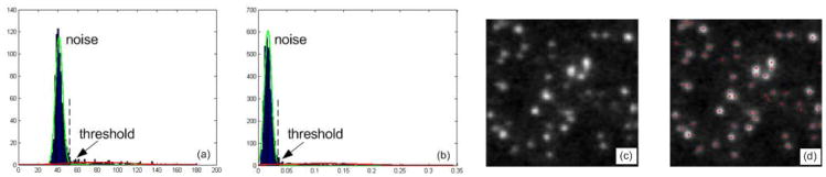
TIRFM is used and clathrin is fluorescently labeled. (a) Histogram of an original image with fitted distributions. (b) Histogram of the local maxima on the filtered image with fitted distributions. (c) A cropped region. (d) The positions of detected CCPs in the region.
Acknowledgments
This work is supported by Keck Foundation.
References
- 1.Slepnev VI, Camilli PD. Accessory factors in clathrin-dependent synaptic vesicle endocytosis. Nature Reviews Neuroscience. 2000;1:161–172. doi: 10.1038/35044540. [DOI] [PubMed] [Google Scholar]
- 2.Brandenburg B, Zhuang X. Virus trafficking - learning from single-virus tracking. Nature Reviews Microbiology. 2007;5:197–208. doi: 10.1038/nrmicro1615. [DOI] [PMC free article] [PubMed] [Google Scholar]
- 3.Yilmaz A, Javed O, Shah M. Object tracking: A survey. ACM Journal of Computing Surveys. 2006;38(4) [Google Scholar]
- 4.Veenman CJ, Reinders MJT, Backer E. Resolving motion correspondence for densely moving points. IEEE Trans on Pattern Analysis and Machine Intelligence. 2001;23(1):54–72. [Google Scholar]
- 5.Carter BC, Shubeita GT, Gross SP. Tracking single-particles: a user-friendly quantitative evaluation. Physical Biology. 2005;2:60–72. doi: 10.1088/1478-3967/2/1/008. [DOI] [PubMed] [Google Scholar]
- 6.Thomann D, Rines DR, Sorger PK, Danuser G. Automatic fluorescent tag detection in 3D with super-resolution: application to the analysis of chromosome movement. J of Microscopy. 2002;208(1):49–64. doi: 10.1046/j.1365-2818.2002.01066.x. [DOI] [PubMed] [Google Scholar]
- 7.Sbalzarini IF, Koumoutsakos P. Feature point tracking and trajectory analysis for video imaging in cell biology. J of Structural Biology. 2005;151:182–195. doi: 10.1016/j.jsb.2005.06.002. [DOI] [PubMed] [Google Scholar]
- 8.Yang G, Matov A, Danuser G. Reliable tracking of large-scale dense particle motion for fluorescent live cell imaging. Proc of IEEE Int Conf Computer Vision and Pattern Recognition. 2005 [Google Scholar]
- 9.Smal I, Niessen WJ, Meijering E. Advanced particle filtering for multiple object tracking in dynamic fluorescence microscopy images. IEEE Int Symposium on Biomedical Imaging: From Nano to Macro. 2007:1048–1051. [Google Scholar]
- 10.Jaqaman K, Loerke D, Mettlen M, Kuwata H, Grinstein S, Schmid SLL, Danuser G. Robust single-particle tracking in live-cell time-lapse sequences. Nature methods. 2008;5:695–702. doi: 10.1038/nmeth.1237. [DOI] [PMC free article] [PubMed] [Google Scholar]
- 11.Zhang B, Zerubia J, Olivo-Marin JC. Gaussian approximations of fluorescence microscope point-spread function models. Applied Optics. 2007;46(10):1819–1829. doi: 10.1364/ao.46.001819. [DOI] [PubMed] [Google Scholar]
- 12.Poore AB, Gadaleta S. Some assignment problems arising from multiple target tracking. Mathematical and Computer Modelling. 2006;43:1074–1091. [Google Scholar]
- 13.Reid DB. An algorithm for tracking multiple targets. IEEE Trans on Automatic Control. 1979;24:843–854. [Google Scholar]
- 14.Rangarajan A, Chui H, Bookstein FL. The softassign procrustes matching algorithm. In: Duncan JS, Gindi G, editors. IPMI 1997 LNCS. Vol. 1230. Springer; Heidelberg: 1997. pp. 29–42. [Google Scholar]
- 15.Kasturi R, et al. Framework for performance evaluation of face, text, and vehicle detection and tracking in video: data, metrics, and protocol. IEEE Trans on Pattern Analysis and Machine Intelligence. 2009;31(2):319–336. doi: 10.1109/TPAMI.2008.57. [DOI] [PubMed] [Google Scholar]