Phase Rotation Methods in Filtering Correlation Coefficients for Ultrasound Speckle Tracking

Abstract

In speckle-tracking-based myocardial strain imaging, large interframe/volume peak-systolic strains cause peak hopping artifacts separating the highest correlation coefficient peak from the true peak. A correlation coefficient filter was previously designed to minimize peak hopping artifacts. For large strains, however, the correlation coefficient filter must follow the strain distribution to remove peak hopping effectively. This processing usually means interpolation and high computational load. To reduce the computational burden, a narrow band approximation using phase rotation is developed in this paper to facilitate correlation coefficient filtering. Correlation coefficients are first phase rotated to increase coherence, then filtered. Rotated phase angles are determined by the local strain and spatial position. This form of correlation coefficient filtering enhances true correlation coefficient peaks in large strain applications if decorrelation due to deformation does not completely destroy the coherence among neighboring correlation coefficients. The assumed strain used in the filter can also deviate from the true strain and still be effective. Further improvement in displacement estimation can be expected by combining correlation coefficient filtering with a new Viterbi-based displacement estimator.

I. Introduction

Tissue velocity imaging (TVI) [1]–[7] and strain rate imaging (SRI) [8]–[22] based on tissue Doppler measurements are 2 primary echocardiographic techniques to detect abnormalities in myocardial contractility. Both exhibit limited sensitivity and spatial resolution, however, because very small deformations must be used to avoid aliasing artifacts. To overcome this problem, multidimensional speckle tracking using RF data has been proposed [23]–[39]. Multidimensional displacements are first estimated from 2 consecutive RF image frames. In this procedure, real RF signals are transformed into complex analytic signals, and then a multidimensional kernel in the first image is correlated to speckle over a search region in the second image to estimate the displacement vector between images at the position of the kernel in the first image. Accurate subpixel axial displacement estimates are obtained using the phase-zero crossing of the complex correlation coefficient in the region of peak correlation.

Multidimensional speckle tracking can overcome many of the limitations of Doppler-based techniques [22]–[26], [30]–[32], [35], [37]. Much larger interframe strains can be processed, resulting in more accurate and precise strain estimates. At conventional frame rates, however, interframe strains at peak systole can still be large enough to induce significant interframe speckle decorrelation. For real-time 3-D data acquisition (i.e., 4-D echocardiography), in which displacement decorrelation due to out-of-plane motion is eliminated, interframe strain magnitudes at peak systole can still produce significant decorrelation at frame rates less than 100 frames per second, as typically used by the current generation of clinical scanners such as the Philips IE33/IU22 (Philips Medical Systems, Bothell, WA). Indeed, intervolume strains as high as 10% can be encountered at peak systole, producing significant peak-hopping artifacts.

Peak hopping refers to the phenomenon in which the nominal correlation coefficient peak is separated from the true peak by an interval representing an integer multiple of the RF carrier period. When used with high interframe strains, multidimensional speckle-tracking algorithms must be adjusted to suppress peak hopping. In [40], correlation coefficient filtering at the same lag was introduced to minimize peak-hopping artifacts at the slight expense of spatial resolution. This processing greatly improves displacement maps at low strain values. At high strain values, however, filtering at constant lag (i.e., vertical filter in correlation space) cannot remove most peak hopping artifacts because the local similarity of the correlation coefficients at the same lag is broken.

In previous papers [41], [42], we analyzed displacement estimation error and presented a 1-D slant filter (i.e., correlation coefficient filter applied along a line tilted in correlation space) to minimize peak hopping artifacts significantly in regions of high strain magnitude. Although the slant filter is highly effective, interpolation during correlation coefficient filtering significantly increases computational burden. Moreover, when the slant correlation coefficient filter is extended to multidimensional speckle tracking, filtering on multiple lag dimensions greatly increases complexity. Therefore, a narrow band approximation, phase rotation, is introduced and applied to speckle tracking in this paper. We present the algorithm in Section II and describe simulations used to test it in Section III. Results are presented in Section IV, and we conclude with a discussion of the results in Section V.

$${\rho }_{mn}(l,k)=\frac{{\displaystyle \sum _{j=-K/2}^{K/2}}{\displaystyle \sum _{i=-L/2}^{L/2}}{W}_{ij}[x(m+i,n+j)y\ast (m+l+i,n+k+j)]}{{\left[{\displaystyle \sum _{j=-K/2}^{K/2}}{\displaystyle \sum _{i=-L/2}^{L/2}}{W}_{ij}{\mid x(m+i,n+j)\mid }^2\right]}^{1/2}{\left[{\displaystyle \sum _{j=-K/2}^{K/2}}{\displaystyle \sum _{i=-L/2}^{L/2}}{W}_{ij}{\mid y(m+l+i,n+k+j)\mid }^2\right]}^{1/2}}$$ (1)

II. Methods

To calculate the correlation coefficient at every pixel, a correlation kernel with extent approximately equal to one speckle around the selected pixel in the predeformed image is defined and then correlated with the postdeformed complex image. The cross correlation coefficient ρ_mn(l,k) pixel (m,n) with lag (l,k) is calculated by (1) (see above) as described in [36], where K and L are the kernel extents in 2 dimensions, respectively; W_ij is the weight within the correlation kernel; x(m,n) is the complex predeformed analytic signal at pixel (m,n); and y(m,n) is the complex postdeformed analytic signal at pixel (m,n).

To improve signal-to-noise ratio and reduce peak-hopping artifacts during cross-correlation coefficient computation, 2-D cross-correlation coefficients are filtered as

$${\widehat{\rho }}_{mn}(l,k)=\sum _{i=-I/2}^{I/2}\sum _{j=-J/2}^{J/2}{F}_{ij}\left[{\rho }_{m+i,n+j}(l,k)\right]$$ (2)

where {F_ij} is the unity gain coefficient of the correlation filter, and I and J are the filter extents in 2 dimensions.

Calculation and filtering of 2-D correlation coefficients can be extended to 3-D as shown in [36]. However, for simplicity, in this paper we first discuss 1-D applications to develop the algorithm and then extend it to 2-D. Future extension to 3-D should be straightforward.

The 1-D displacement of a pixel as a function of time under constant strain can be formulated as:

$${\tau }_d=\epsilon t+{\tau }_0$$ (3)

where τ_d is the displacement at time t (depth d = ct/2, where c is the speed of sound), t is the propagation time (depth), τ₀ is the common displacement (translation), and ε is the strain.

For discrete signals, the 1-D correlation coefficient ρ_n(l) at time n with lag l is written as:

$${\rho }_n(l)=\frac{{\displaystyle \sum _{i=-L/2}^{L/2}}{W}_{i}x(n+i)y^{\ast }(n+i+l)}{{\left[{\displaystyle \sum _{i=-L/2}^{L/2}}{W}_i{\mid x(n+i)\mid }^2\right]}^{1/2}{\left[{\displaystyle \sum _{i=-L/2}^{L/2}}{W}_i{\mid y(n+i+l)\mid }^2\right]}^{1/2}}.$$ (4)

The original correlation coefficient filter in [40] is presented as

$${\widehat{\rho }}_n(l)=\sum _{m=-M/2}^{M/2}h(m){\rho }_{n+m}(l)$$ (5)

where n is the nth pixel of the correlation coefficient, W_i is the weight within the correlation kernel, M is the extent of the cross correlation coefficient filter, h is the cross correlation coefficient filter, ρ is the unfiltered correlation coefficient, and ρ̂ is the filtered correlation coefficient.

The filter is along the space/time direction but with constant lag. However, to maintain coherence for correlation-coefficient filtering, the filter should not be applied along a vertical line, but rather along a line matching the local strain. To illustrate this point, we present the magnitude and phase of the complex correlation coefficients for the 1-D simulation described in the next section, as a function of depth (vertical) and lag/displacement (horizontal) in Fig. 1. A vertical filter is depicted by the blue (vertical) line and a slant filter by the red (slanted) line. Clearly, a slant filter better maintains coherence across the filter dimension.

Fig. 1.

The (a) amplitude and (b) phase angle of the estimated correlation coefficient in 1-D simulation. The blue vertical line is the direction of the vertical correlation coefficient filter and the red diagonal line is the direction of the slant correlation coefficient filter. References to color refer to the online version of this figure.

That is, the correlation-coefficient filtering now takes the form

$${\widehat{\rho }}_n=(l)\sum _{m=-M/2}^{M/2}h(m){\rho }_{n+m}(\epsilon m+l)$$ (6)

where M is the extent of the correlation filter. Because correlation-coefficient filtering is along the distribution of strain, it is called the slant filter.

Interpolation is needed because εm is usually not an integer number. This increases the computational burden. A possible simplification can be obtained if the analytical signal can be represented as a narrow band approximation.

$${\rho }_n(l)=A_n(l\mathrm{\Delta }t)e^{-j\omega l\mathrm{\Delta }t}$$ (7)

where ω is the central frequency of the ultrasound signal, Δt is the sampling time interval, and A_n(lΔt) is the envelope of the cross-correlation function at the nth pixel.

Introducing (7) into (6), (6) is modified as

$$\begin{array}{l}{\widehat{\rho }}_n(l)=\sum _{m=-M/2}^{M/2}h(m){\rho }_{n+m}(\epsilon m+l)\\ =\sum _{m=-M/2}^{M/2}h(m)A_{n+m}(\epsilon m+l)e^{-j\omega (\epsilon m+l)\mathrm{\Delta }t}.\end{array}$$ (8)

As shown Fig. 1(a), A_n+m(εm + l) is the amplitude of the cross-correlation coefficient. In regions around real peaks of the cross-correlation coefficient, A_n+m(εm + l) can be approximated as A_n+m(l); thus, the equation can be furthered simplified as

$$\begin{array}{l}{\widehat{\rho }}_n(l)=\sum _{m=-M/2}^{M/2}h(m)A_{n+m}(l)e^{-j\omega l\mathrm{\Delta }t}{e}^{-j\omega \epsilon m\mathrm{\Delta }t}\\ =\sum _{m=-M/2}^{M/2}h(m){\rho }_{n+m}(l)e^{-j\omega \epsilon m\mathrm{\Delta }t}.\end{array}$$ (9)

As shown in (9), the slant correlation coefficient filter is approximated as a vertical correlation coefficient filter, in which the lag of the correlation coefficients is constant, after multiplying correlation coefficients at the same displacement with a phasor determined by the applied strain and the location of the correlation kernel. This procedure is similar to phase rotation in beamforming [43], and rotated signals are phase coherent. It is called “tilt filter” in this paper to differentiate it from slant filter in [41], and the original correlation-coefficient filtering process in [40] is called “filter” or “vertical filter” for simplicity.

The tilt filter technique can be extended to both 2 and 3 dimensions. In 2-D applications, vertical cross correlation coefficient filtering is

$${\widehat{\rho }}_{m_0{n}_0}(l,k)=\sum _{n=-N/2}^{N/2}\sum _{m=-M/2}^{M/2}h(m,n){\rho }_{(m_0+m)(n_0+n)}(l,k)$$ (10)

where m₀ is in the lateral direction of the ultrasound beam, n₀ is in the axial direction of the ultrasound beam, M is the lateral extent of correlation-coefficient filtering, N is the axial extent of correlation-coefficient filtering, m is the axial shift of correlation-coefficient filtering, and n is the lateral shift of correlation-coefficient filtering.

A general deformation in either 2 or 3 dimensions has both normal and shear components. Because spatial frequencies in the axial direction are so much higher than those in either lateral or elevational directions [44], decorrelation is dominated by the partial derivatives of the axial displacement with respect to all directions, where the displacement vector v = (u,v,w) and the propagation direction is along the y (v) axis. In 2-D, this means the partial derivative of the axial displacement v with respect to the lateral direction x (ε₁ = ∂v/∂x) and the partial derivative of the axial displacement v with respect to the axial direction y (ε₂ = ∂v/∂y) are the primary sources of decorrelation. In 3-D, the partial derivative of the axial displacement with respect to the elevational displacement must also be considered. Note that only the axial term in the symmetric shear strain [ε_xy = 1/2(∂u/∂y + ∂v/∂x)] contributes significantly to decorrelation. This means that rotations as well as deformations can produce decorrelation through the same mechanism. Using these definitions and the approximation that decorrelation is produced only by spatial variations in the axial displacement, tilt filtering in 2-D becomes:

$${\widehat{\rho }}_{m_0{n}_0}(l,k)=\sum _{m=-M/2}^{M/2}\sum _{n=-N/2}^{N/2}h(m,n){\rho }_{m_0+m{n}_0+n}(l,k)e^{-j{\omega }_c({\epsilon }_{1}m\mathrm{\Delta }{t}_x+{\epsilon }_{2}n\mathrm{\Delta }{t}_y)}$$ (11)

where Δt_x and Δt_y are the lateral and axial sampling distances, respectively; ε₁ = ∂v/∂x and ε₂ = ∂v/∂y are the partial derivatives of the axial displacement with respect to lateral and axial directions, respectively; and ω_c is the central frequency of the ultrasound signal in the axial direction.

Note that Δt_x is usually much greater than Δt_y, and the spatial extent of the correlation kernel and filter are significantly larger in the lateral direction. This means that an equal displacement gradient across the beam direction produces significantly more decorrelation than that along the beam direction, and tilt filtering in the lateral direction becomes more important than tilt filtering in the axial direction.

III. Simulations

A. 1-D Simulation

1-D simulations were first designed to verify the algorithm. Point scatterers were randomly distributed along a 4 cm distance. A pulse with 5 MHz central frequency and 50% fractional bandwidth was convolved with the scatterers to generate a predeformed RF signal. Scatterers were then compressed and a postdeformed RF signal was generated. White noise was added to both RF signals with an SNR of 40 dB. Four different constant strains, −7, −8, −9, and −10%, were used for compression. RF signals were sampled at a 20 MHz rate. In the correlation calculation, the kernel was selected as one speckle size of the RF signal, or approximately 0.41 mm, and the correlation filter length was chosen as 3 times the speckle size, or approximately 1.21 mm.

Complex correlation coefficients at the same depth are all multiplied with the phasor defined in (9), where a strain value must be assumed before phase rotation. In this application, we first applied the simulated strain value and then varied the assumed strain to test the robustness of tilt filtering.

To show the performance of the tilt filter, for each strain value, the simulation was repeated for 200 iterations, in which both vertical filtering and tilt filtering were applied. The estimated displacement at a sample volume was compared with the actual displacement. A peak-hopping artifact was identified if the difference in time between estimated and actual displacements is larger than 2 counts of the sampling period.

B. 2-D simulation

A simplified 2-D model simulating a hard inclusion in a soft medium presented in [45] was used to predict lateral and axial displacement according to the following equations.

$$\begin{array}{l}u=\frac{x}{r}\left(\frac{x^2}{r^2}Q(r)+\frac{y^2}{r}\frac{\partial Q(r)}{\partial r}\right)\\ v=-\frac{y}{r}\left(\frac{y^2}{r^2}Q(r)+\frac{x^2}{r}\frac{\partial Q(r)}{\partial r}\right)\end{array}$$ (12)

and Q(r) is defined as

$$\begin{array}{ll}Q(r)=P\frac{2}{1+K}r,\hfill & r\le R\hfill \\ Q(r)=P\left[1+\frac{1-K}{1+K}\left(2\frac{R^2}{r^2}-\frac{R^4}{r^4}\right)\right]r,\hfill & r>R\hfill \end{array}$$ (13)

where r is the distance between a sample volume and the center of the coordinate system, and $r=\sqrt{x^2+y^2}$; P is a deformation scalar related to the magnitude of the applied force; R is the radius of the hard inclusion centered in the medium; K is the ratio of the Young’s modulus of the hard inclusion to that of the background soft medium; and u and v are the lateral and axial displacements, respectively, for r ≤ R, u = [2/(1 + K)]Px and v = [2/(1 + K)]Py.

The medium is 40 mm × 40 mm, where a 10 mm diameter inclusion 6 times harder than the background medium (K = 6) was located at the center. Scatterers were distributed uniformly (with density of 0.75 scatterers per sample interval), and their amplitudes obey a Rayleigh distribution to generate a fully developed speckle pattern [46]. A point spread function with a 5 MHz central frequency, 0.25 mm axial full-width-half-maximum (FWHM), and 0.5 mm lateral FWHM was convolved with the scatterer distribution to generate predeformation and postdeformation ultrasound RF fields corresponding to scatterer locations before and after deformation. Simulated lateral and axial displacements are shown in Fig. 2, and corresponding ε₁ and ε₂ strain distributions are shown in Fig. 3 for an average strain of −8%. A correlation kernel 0.42 mm axially by 1.5 mm laterally, slightly larger than one speckle spot, was used to calculate correlation coefficients. The correlation coefficient filter was 0.84 mm axially by 2.1 mm laterally, representing about 2 speckle spots.

Fig. 2.

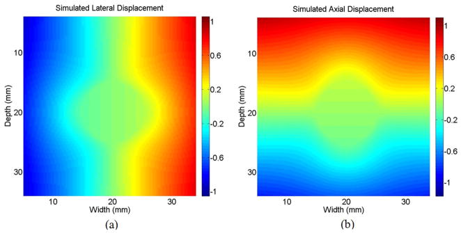
(a) Lateral and (b) axial displacement used in 2-D simulation (K = 6).

Fig. 3.

Simulated strain distribution of (a) ε₁ = (dv/dx) and (b) ε₂ = (dv/dy), where dv means the axial displacement difference between the adjacent sample volumes, dx means the lateral distance between the adjacent sample volumes, and dy means the axial distance between the adjacent sample volumes. This is the initial input to the tilt filter.

Correlation coefficients were multiplied with the phasor defined in (11) according to the local derivatives of axial displacement with respect to axial and lateral dimensions. Integer displacements were estimated based on the locations of peak values of filtered/tilt filtered correlation coefficients. These coarse measures were further refined using a lateral synthetic phase algorithm on both filtered and tilt-filtered correlation coefficients to estimate axial and lateral displacements concurrently [45]. Similarly, strain components with respect to axial displacement were calculated based on estimated displacements from vertical and tilt filtering.

IV. Results

The amplitude and phase of correlation coefficients for the 1-D simulation are presented in Fig. 1 for an applied strain of −7%. Again, the blue line is the direction of the vertical correlation coefficient filter and the red line is the direction of the slant-correlation-coefficient filter. These same data are presented in Fig. 4, but with phase rotation applied according to (8) assuming −7% strain. Clearly, the phase of the correlation coefficient is locally aligned so that a vertical filter will highlight regions of strong correlation.

Fig. 4.

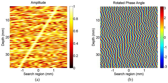
The (a) amplitude and (b) rotated phase angle of the correlation coefficient in 1-D simulation.

The correlation coefficients in Figs. 1 and 4 were filtered using a vertical correlation filter. Fig. 5 presents results without phase rotation of Fig. 1, and Fig. 6 presents equivalent results with phase rotation. As expected, tilt filtering greatly enhances regions of high correlation in this high strain case.

Fig. 5.

The (a) amplitude and (b) phase angle of the filtered correlation coefficient in 1-D simulation.

Fig. 6.

The (a) amplitude and (b) phase angle of the tilt-filtered correlation coefficient in 1-D simulation.

Estimated displacements for the 1-D simulation at −7% strain using tilt filtering, shown in Fig. 7(a), are compared with those using vertical filtering, shown in Fig. 7(b). Peak hopping is eliminated for tilt filtering with the correct strain value. However, vertical filtering produces significant peak hopping artifacts because the small strain assumption of [40] is violated.

Fig. 7.

Estimated displacement using the (a) tilt filter and (b) filter for −7% strain.

In Fig. 8, we present examples of estimated results at different large strain values ranging from −7% to −10% using the correct strain value for tilt filtering. The ratio of peak-hopping artifacts to total results is summarized for all 1-D simulations in Table I. Note that at −9% strains, significant peak-hopping artifacts appear even for tilt filtering. Nevertheless, peak hopping is greatly reduced at all strain levels for tilt filtering compared with vertical filtering.

Fig. 8.

Comparison of estimated displacements for (a) −7%, (b) −8%, (c) −9%, and (d) −10% strains.

TABLE I.

Percentage of Peak Hopping Errors Using Tilt and Vertical Filtering.

Strain value	Tilt filtering with right assumed strain value	Vertical filtering
−7%	0.07%	88.20%
−8%	0.11%	96.74%
−9%	2.01%	99.13%
−10%	4.73%	99.70%

Estimated displacements for the 2-D simulation using only vertical filtering are shown in Figs. 9(a) and (b). Relating the results to the simulated strain distribution, peak-hopping errors dominate in regions with high ε₁ (∂v/∂x) and ε₂ (∂v/∂y), which are localized at ±45 degree, ±135 degree corners of the inclusion. Estimated displacements using tilt filtering are shown in Figs. 9(c) and (d). Assumed strains for filtering were the actual strains at each pixel. Peak-hopping errors are almost completely eliminated for tilt filtering, except for a few points in the high-strain corner positions. Here, the absolute value of the correlation coefficient is very low due to the high strains. Consequently, filtering, even tilt filtering, is still subject to peak hopping because the absolute value of the correlation coefficient remains low after filtering.

Fig. 9.

The estimated (a) lateral displacement and (b) axial displacement using filtered speckle tracking, and the estimated (c) lateral displacement and (d) axial displacement using tilt-filtered speckle tracking.

Following displacement estimation, strains were obtained from derivatives of the displacements using a least squares fitting method [47]. The strain components estimated from the results of vertical filtering are shown in Figs. 10(a) and (b), and strain values estimated from the results of tilt filtering are shown in Figs. 10(c) and (d). Clearly, significant peak-hopping artifacts dominate vertical filtered results. In contrast, tilt filtering produces much more stable results except in small regions with low absolute correlation coefficients located at the ±45 degree and ±135 degree corners of the inclusion.

Fig. 10.

Estimated strain distribution of (a) ε₁ = (dv/dx), and (b) ε₂ = (dv/dy) using nontilt filter, where dv means axial displacement between adjacent sample volumes, dx means lateral distance between adjacent sample volumes, and dy means axial distance between adjacent sample volumes. Estimated (c) strain distribution of ε₁ = (dv/dx) and (d) ε₂ = (dv/dy) using tilt filter.

Although the primary objective of the tilt-correlation-coefficient filter is to eliminate peak hopping at extremely high strains, we also observed that the SNR of lateral displacement estimates improved over a wide range of applied strains. For example, in low strain regions of Fig. 9 without peak-hopping artifacts, the SNR of estimated lateral displacements clearly improved with tilt filtering. To further demonstrate this effect, 3 simulations with average applied strains of −0.5, −1, and −2% were performed using the same model as Section II. Estimated lateral displacements results using vertical filtering and tilt filtering are contrasted in Fig. 11. The SNR improvement (Table II) is calculated as the ratio of the average estimated variance over the entire image field for vertical filtering to the estimated variance for tilt filtering. Tilt filtering improves lateral displacement estimation primarily because coherence is better preserved across the filter dimension. This means the 2nd moment of the filtered-correlation-coefficient function is smaller in the lateral direction. The smaller the 2nd moment is, the smaller the variance because lateral displacement is usually estimated by parabolic fitting on the correlation coefficient function.

Fig. 11.

Estimated lateral displacements using (a) correlation coefficient filter and (b) tilt correlation coefficient filter for average −0.5% strain; estimated lateral displacements using (c) correlation coefficient filter and (d) tilt correlation coefficient filter for average −1% strain; estimated lateral displacements using (e) correlation coefficient filter and (f) tilt correlation coefficient filter for average −2% strain.

TABLE II.

SNR Improvement of Lateral Displacement at Different Strains (10 log₁₀ (variance ratio)).

	−0.5%	−1%	−2%
SNR improvement	0.57 dB	3.11 dB	3.93 dB

V. Discussion and Conclusion

Vertical filtering in correlation space can increase contrast near the peak correlation coefficient at low strains. At high strains, however, contrast is actually lost because phase coherence is not maintained across the filter. In contrast, tilt filtering rotates the phase of the correlation coefficient function before filtering to maintain coherence over the filter dimension. Tilt filtering approximates the coherent sum over correlation coefficients assuming that correlation coefficients corresponding to peak-hopping artifacts do not have neighboring coherent correlation coefficients.

Peak values of tilt-filtered correlation coefficients are usually lower than those of unfiltered ones, but the contrast in tilt-filtered correlation coefficients at real displacements is usually enhanced compared with that at peak hops. For large strain applications, vertical-filtered correlation coefficients are distorted, producing significant peak-hopping artifacts. As the results presented in Figs. 5 and 6 clearly show, tilt filtering can greatly increase contrast in the correlation-coefficient function at strains where vertical filtering actually reduces contrast compared with unfiltered results.

Speckle can decorrelate due to electronic noise, displacements out of the image line/plane (not significant for 3-D tracking), deformations, and rotations. In the present study, we have only considered decorrelation due to deformations. We note, however, that variations in the axial displacement across the beam direction due to deformations in 2-D simulations are equivalent to variations in the axial displacement across the beam direction due to rotations of the same magnitude. In deformation-limited speckle tracking, the main source of decorrelation is the redistribution of ultrasonic scatterers within the resolution cell due to the deformation.

To explore the strain limits of tilt filtering, we have developed a simple decorrelation model. If a large deformation produces significant decorrelation within the resolution cell itself, than no amount of filtering will restore full coherence to the correlation coefficient function. For the 1-D case, the model assumes pure deformation without bulk translation. To simplify the problem, the incident pulse is formulated in continuous time as p(t) = e^jω₀t, t ∈ [−T/2, T/2], with uniform amplitude, linear phase, and limited pulse length T representing one speckle length. The incident pulse is convolved with a reflector function σ(t) to generate the received signal s(t). The direction of deformation is parallel to wave propagation so the only strain component is the normal strain with respect to axial displacement. Assuming the strain is ε, the predeformed received signal is

$$s_1(t)=p(t)\ast \sigma (t)=a(t)e^{j{\omega }_{0}t}$$ (14)

and the postdeformed signal is

$$s_2(t)=p(t)\ast \sigma (t(1+\epsilon ))=a(t(1+\epsilon ))e^{j{\omega }_0(1+\epsilon )t}.$$ (15)

The cross-correlation coefficient is calculated in continuous time as

$$\rho (\tau )=\frac{E\left({\int }_{-T/2}^{T/2}{s}_1^{\ast }(t^{\prime }+\tau )s_2(t^{\prime }){dt}^{\prime }\right)}{\sqrt{E\left({\int }_{-T/2}^{T/2}{|s_1(t^{\prime })|}^2{dt}^{\prime }\right)E\left({\int }_{-T/2}^{T/2}{|s_2(t^{\prime })|}^2{dt}^{\prime }\right)}}$$ (16)

and the peak cross-correlation coefficient appears at τ = 0. Therefore,

$$\rho (0)\approx \frac{E\left({\int }_{-T/2}^{T/2}(a(t^{\prime })a(t^{\prime }(1+\epsilon )))e^{j{\omega }_0\epsilon t^{\prime }}{dt}^{\prime }\right)}{\sqrt{E\left({\int }_{-T/2}^{T/2}a{(t^{\prime })}^2{dt}^{\prime }\right)E\left({\int }_{-T/2}^{T/2}a{((1+\epsilon )t^{\prime })}^2{dt}^{\prime }\right)}}.$$ (17)

We simplify further assuming the envelope a(t) is constant in [−T/2, T/2] and the integration can be approximated as

$$\begin{array}{l}\rho (0)=\frac{\underset{-T/2}{\overset{T/2}{\int }}{e}^{j\epsilon {\omega }_0{t}^{\prime }}{dt}^{\prime }}{T}=\frac{e^{j\epsilon {\omega }_{0}T/2}-e^{-j\epsilon {\omega }_{0}T/2}}{j{\omega }_{0}T}\\ =\frac{sin\left(\epsilon {\omega }_{0}T/2\right)}{\epsilon {\omega }_{0}T/2}=\text{sinc}\left(\epsilon {\omega }_{0}T/2\right).\end{array}$$ (18)

The peak value of the cross-correlation coefficient versus normal strain can be estimated using this equation. If the fractional bandwidth of the emitted ultrasound signal is 50%, one speckle would extend 2 cycles of the carrier frequency. The peak value of the cross-correlation coefficient is estimated as sinc(2πε) according to (18), and it is presented as a function of normal strain and shown as the blue solid line in Fig. 12. Similar decorrelation models were published in [48] and [49]. A sinc decorrelation function is also shown in [48] and compares reasonably well with experimental and simulated results.

Fig. 12.

The peak cross-correlation coefficient amplitude for normal strain (blue solid line) and shear strain (red dash line). References to color refer to the online version of this figure.

Similarly, decorrelation in 2-D can be analyzed by looking at changes in speckle patterns due both to axial normal strain (i.e., ε₂), and gradients in the axial displacement perpendicular to the propagation direction (i.e., ε₁ or axial shear strain). Along the beam direction, (18) still applies. Across the beam direction, considering plane wave propagation in the far field, the wavefront travels an interval t in time on one side and 2ε₁t more on the other side because of the 2-way roundtrip of ultrasound wave propagation. A simple approximation leads to the same form laterally as (17) considering the beam to be of constant amplitude over a width determined by the product of the wavelength and the f/number of the imaging aperture. The integration extent in the lateral equivalent of (16) is determined by the beam width and the phase term of the integrand is replaced as e^{j₂ω₀ε₁t′}. For a system with an f/number of 2, the peak value in (18) is ρ(0) = sinc(2ε × 2 × 2π)/2 = sinc(4πε₁). The peak cross-correlation coefficient versus ε₁ is shown as the red dash line in Fig. 12. Note that this function decorrelates faster, even for a high-quality f/2 imaging system. In clinical applications, especially in echocardiography, much higher f/numbers are usually used resulting in significantly higher decorrelation due to ε₁ (and rotations producing equivalent ε₁) rather than ε₂.

In real 2-D applications, decorrelation is worse than both curves in Figs. 12(a) and (b) because the cross correlation is calculated throughout the whole speckle spot instead of just in axial or lateral directions. Decorrelation is closely related to peak hopping. For example, in the 2-D simulation presented here, both ε₁ and ε₂ were large at the ±45 degree, ±135 degree corners of the inclusion, resulting in significant decorrelation and peak-hopping artifacts.

Fig. 13 presents results of the 1-D simulation at strains of −12% and −15% before any filtering. Note that the magnitudes of the correlation coefficient are greatly distorted at these high strain values—the tilted constant strain curve is hard to identify in the amplitude plots. No form of filtering will uniformly eliminate potential peak-hopping artifacts in this case. It is interesting to note, however, that the tilted constant strain curve is still apparent in the phase plots. Rotation by the correct phase tilt still produces vertical phase curves in the region of true displacements. Consequently, if the approximate position of the correlation peak can be estimated by other means, then the displacement can still be accurately estimated using the phase zero-crossing method. This possibility is explored in a subsequent publication.

Fig. 13.

The (a) amplitude, (b) phase angle, and (c) rotated phase angle of the calculated correlation coefficient in simulation of −12% strain. The (d) amplitude, (e) phase angle, and (f) rotated phase angle of the correlation coefficient in 1-D simulation of −15% strain. The blue dash line shows the actual displacement versus depth in panels (a) and (d). References to color refer to the online version of this figure.

A strain value must be assumed before tilt filtering; however, the strain value is unknown unless some other information can be used to estimate local displacements. As a simple test of tilt filtering robustness to errors in the strain estimate, we repeated the 1-D simulation for values of the assumed strain not equal to the actual strain. Four plots in Fig. 14 show estimated displacements when the real strain is −7% but the assumptions are −4, −6, −8, and −10%, respectively, in Fig. 14(a)–(d). Even if the assumed strain does not equal the real strain, displacement estimation is still better than assuming no strain (i.e., vertical filtering; compare with Fig. 7). Also, note that overassumption is better than underassumption in our simulation of compression. The reason is that in tilt filtering, the phase is rotated but the amplitude is not. For compression, the correlation coefficient with overassumed strain (i.e., assumed strain magnitude greater than the actual strain magnitude) is more coherent than that with underassumed strain. Furthermore, it is reasonable that underassumed strain (i.e., assumed strain magnitude less than the actual strain magnitude) works better in the simulation of expansion. For precise estimation, an iterative process is needed to refine the assumed strain at each step of tilt filtering using the estimated displacement of the previous step.

Fig. 14.

Estimated displacement with strain assumptions of (a) −4%, (b) −6%, (c) −8%, and (d) −10%, where the actual strain is −7% in all 4 simulations. Assumed strains were input to tilt filters to produce these results.

A practical concern for this iterative process is estimating the initial strain value. Presumably, initial strain guesses must be obtained from displacement estimates using either unfiltered or vertically filtered correlation coefficients. Our group has developed a displacement estimator based on Viterbi processing of unfiltered correlation coefficients to estimate local displacements [50] to have reasonable initial guesses needed to seed an iterative tilt-filtering algorithm properly.

In summary, to eliminate peak-hopping errors during large strain estimation, a correlation-coefficient filter matching the strain distribution was presented. It uses the phase coherence between neighboring correlation coefficients and thereby improves the accuracy and precision of displacement estimation. This algorithm is restricted by decorrelation due to deformation. The assumed initial strain does not need to equal the real strain, and an iterative approach can be used to improve calculated strains where the displacements from one iteration are used to compute the assumed strains for the next iteration.

Biographies

Lingyun Huang received a B.S. degree in biomedical engineering from Zhejiang University in 1997, an M.S. degree in pattern recognition and artificial intelligence from the Institute of Automation, Chinese Academy of Science in 2000, and a Ph.D. degree in bioengineering from the Department of Bioengineering, University of Washington, Seattle.

He is currently a postdoctoral research fellow in the Department of Bioengineering at the University of Washington. His research interests include ultrasound elasticity imaging, signal processing, and image processing.

Yael Petrank was born in Haifa, Israel. She received a B.Sc. degree in physics from the Technion—Israel Institute of Technology, Haifa, Israel, and an M.Sc. degree and a Ph.D. degree from the Biomedical Engineering Department at the Technion. She then worked as a physicist for Insightec, as an algorithmic developer in Mediguide, and as a senior fellow in the Department of Bioengineering at the University of Washington in Seattle. Yael is currently working as a senior research associate at the Biomedical Engineering Faculty in the Technion, focusing on segmentation of cardiac ultrasound images

Sheng-Wen Huang was born in 1971 in Changhua, Taiwan, R.O.C. He received the B.S. and Ph.D. degrees from National Taiwan University, Taipei, Taiwan, R.O.C., in 1993 and 2004, respectively, both in electrical engineering. He worked as a postdoctoral researcher at National Taiwan University from 2004 to 2005 and is currently a postdoctoral researcher with the Department of Biomedical Engineering at the University of Michigan, Ann Arbor. His current research interests include optoacoustic transduction and imaging, ultrasound elasticity imaging, and thermal strain imaging.

Congxian Jia received the B.S. degree and an M.S. degree in mechanical engineering from Beijing University, Beijing, P. R. C., in 1999 and 2002, respectively. She also received an M.S. degree in biomechanics of aerospace and mechanical engineering in 2004 from Boston University, Boston, MA.

She is currently a Ph.D. candidate at the University of Michigan, Ann Arbor, working as a research assistant in the Biomedical Ultrasonics Laboratory. She is a student member of the IEEE. Her research interests include ultrasound elasticity imaging and its applications to cardiac diagnosis.

Matthew O’Donnell (M’79–SM’84–F’93) received a B.S. degree and a Ph.D. degree in physics from the University of Notre Dame, Notre Dame, IN, in 1972 and 1976, respectively.

Following his graduate work, Dr. O’Donnell moved to Washington University in St. Louis, MO, as a postdoctoral fellow in the Physics Department working on applications of ultrasonics to medicine and nondestructive testing. He subsequently held a joint appointment as a senior research associate in the Physics Department and a research instructor of medicine in the Department of Medicine at Washington University. In 1980, he moved to the General Electric Corporate Research and Development Center in Schenectady, NY, where he continued to work on medical electronics, including MRI and ultrasound imaging systems. During the 1984–1985 academic year, he was a visiting fellow in the Department of Electrical Engineering at Yale University in New Haven, CT, investigating automated image analysis systems. In 1990, Dr. O’Donnell became a professor of electrical engineering and computer science at the University of Michigan in Ann Arbor, MI. Starting in 1997, he held a joint appointment as professor of biomedical engineering. In 1998, he was named the Jerry W. and Carol L. Levin Professor of Engineering. From 1999 to 2006, he also served as chair of the Biomedical Engineering Department. During 2006, he moved to the University of Washington in Seattle, WA, where he is now the Frank and Julie Jungers Dean of Engineering and also a professor of bioengineering. His most recent research has explored new imaging modalities in biomedicine, including elasticity imaging, in vivo microscopy, optoacoustic arrays, optoacoustic contrast agents for molecular imaging and therapy, thermal strain imaging, and catheter-based devices.

References

- 1.McDicken WN, Sutherland GR, Moran CM, Gordon LN. Colour Doppler velocity imaging of the myocardium. Ultrasound Med Biol. 1992;18(6):651–654. doi: 10.1016/0301-5629(92)90080-t. [DOI] [PubMed] [Google Scholar]
- 2.Sutherland GR, Stewart MJ, Groundstroem KWE. Color Doppler myocardial imaging: A new technique for assessment of myocardial function. J Am Soc Echocardiogr. 1994 Sep-Oct;7:441–458. doi: 10.1016/s0894-7317(14)80001-1. [DOI] [PubMed] [Google Scholar]
- 3.Kanai H, Koiwa Y, Zhang JP. Real-time measurements of local myocardium motion and arterial wall thickening. IEEE Trans Ultrason Ferroelectr Freq Control. 1999 Sep;46(5):1229–1241. doi: 10.1109/58.796128. [DOI] [PubMed] [Google Scholar]
- 4.Fleming AD, Xia X, McDicken WN, Sutherland GR, Fenn L. Myocardial velocity gradients detected by Doppler imaging. Br J Radiol. 1994 Jul;67:679–688. doi: 10.1259/0007-1285-67-799-679. [DOI] [PubMed] [Google Scholar]
- 5.Uematsu M, Miyatake K, Tanaka N, Matsuda H, Sano A, Yamazaki N, Hirama M, Yamagishi M. Myocardial velocity gradient as a new indicator of regional left ventricular contraction: Detection by a two-dimensional tissue Doppler imaging technique. J Am Coll Cardiol. 1995 Jul;26(1):217–223. doi: 10.1016/0735-1097(95)00158-v. [DOI] [PubMed] [Google Scholar]
- 6.Palka P, Lange A, Fleming AD, Donnelly JE, Dutka DP, Starkey IR, Shaw TRD, Sutherland GR, Fox KAA. Differences in myocardial velocity gradient measured throughout the cardiac cycle in patients with hypertrophic cardiomyopathy, athletes and patients with left ventricular hypertrophy due to hypertension. J Am Coll Cardiol. 1997 Sep;30:760–768. doi: 10.1016/s0735-1097(97)00231-3. [DOI] [PubMed] [Google Scholar]
- 7.Tsutsui H, Uematsu M, Shimizu H, Yamagishi M, Tanaka N, Matsuda H, Miyatake K. Comparative usefulness of myocardial velocity gradient in detecting ischemic myocardium by a dobutamine challenge. J Am Coll Cardiol. 1998 Jan;31:89–93. doi: 10.1016/s0735-1097(97)00430-0. [DOI] [PubMed] [Google Scholar]
- 8.Heimdal A, Stoylen A, Torp H, Skjaerpe T. Real-time strain rate imaging of the left ventricle by ultrasound. J Am Soc Echocardiogr. 1998 Nov;11:1013–1019. doi: 10.1016/s0894-7317(98)70151-8. [DOI] [PubMed] [Google Scholar]
- 9.Stoylen A, Heimdal A, Bjornstad K, Torp H, Skjaerpe T. Strain imaging by ultrasound in the diagnosis of regional dysfunction of the left ventricle. Echocardiography. 1999;16(4):323–329. doi: 10.1111/j.1540-8175.1999.tb00821.x. [DOI] [PubMed] [Google Scholar]
- 10.Voigt JU, Arnold MF, Karlsson M, Hubbert L, Kukulski T, Hatle L, Sutherland GR. Assessment of regional longitudinal myocardial strain rate derived from Doppler myocardial imaging indices in normal and infarcted myocardium. J Am Soc Echocardiogr. 2000 Jun;13:588–598. doi: 10.1067/mje.2000.105631. [DOI] [PubMed] [Google Scholar]
- 11.O’Donnell M, Skovoroda AR, Shapo BM. Measurement of wall motion using Fourier based speckle tracking algorithms. Proc. IEEE 1991 Ultrasonics Symp; Dec. 8–11, 1991; pp. 1101–1104. [Google Scholar]
- 12.Konofagou EE, D’hooge J, Ophir J. Myocardial elastography—A feasibility study in vivo. Ultrasound Med Biol. 2002 Apr;28(4):475–482. doi: 10.1016/s0301-5629(02)00488-x. [DOI] [PubMed] [Google Scholar]
- 13.D’hooge J, Heimdal A, Jamal F, Kukulski T, Bijnens B, Rademakers F, Hatle L, Suetens P, Sutherland GR. Regional strain and strain rate measurements by cardiac ultrasound: Principles, implementation and limitations. Eur J Echocardiogr. 2000 Dec;1:295–299. doi: 10.1053/euje.2000.0031. [DOI] [PubMed] [Google Scholar]
- 14.D’hooge J, Bijnens B, Thoen J, Van de Werf F, Sutherland GR, Suetens P. Echocardiographic strain and strain-rate imaging: A new tool to study regional myocardial function. IEEE Trans Med Imaging. 2002 Sep;21(9):1022–1030. doi: 10.1109/TMI.2002.804440. [DOI] [PubMed] [Google Scholar]
- 15.Sutherland GR, Di Salvo G, Claus P, D’hooge J, Bijnens B. Strain and strain rate imaging: A new clinical approach to quantifying regional myocardial function. J Am Soc Echocardiogr. 2004 Jul;17(7):788–802. doi: 10.1016/j.echo.2004.03.027. [DOI] [PubMed] [Google Scholar]
- 16.Migrino RQ, Zhu XG, Pajewski N, Brahmbhatt T, Hoffmann R, Zhao M. Assessment of segmental myocardial viability using regional 2-dimensional strain echocardiography. J Am Soc Echocardiogr. 2007 Apr;20(4):342–351. doi: 10.1016/j.echo.2006.09.011. [DOI] [PubMed] [Google Scholar]
- 17.D’hooge J, Konofagou E, Jamal F, Heimdal A, Barrios L, Bijnens B, Thoen J, Van de Werf F, Sutherland GR, Suetens P. Two-dimensional ultrasonic strain rate measurement of the human heart in vivo. IEEE Trans Ultrason Ferroelectr Freq Control. 2002 Feb;49(2):281–286. doi: 10.1109/58.985712. [DOI] [PubMed] [Google Scholar]
- 18.Li Y, Garson CD, Xu Y, Beyers RJ, Epstein FH, French BA, Hossack JA. Quantification and MRI validation of regional contractile dysfunction in mice post myocardial infarction using high resolution ultrasound. Ultrasound Med Biol. 2007 Jun;33(6):894–904. doi: 10.1016/j.ultrasmedbio.2006.12.008. [DOI] [PMC free article] [PubMed] [Google Scholar]
- 19.Støylen A, Ingul CB, Torp H. Strain and strain rate parametric imaging. A new method for post processing to 3-/4-dimensional images from three standard apical planes. Preliminary data on feasibility, artefact and regional dyssynergy visualization. Cardiovasc Ultrasound. 2003 Aug;1 doi: 10.1186/1476-7120-1-11. [DOI] [PMC free article] [PubMed] [Google Scholar]
- 20.Pellerin D, Sharma R, Elliott P, Veyrat C. Tissue Doppler, strain, and strain rate echocardiography for the assessment of left and right systolic ventricular function. Heart. 2003;89(suppl III):9–17. doi: 10.1136/heart.89.suppl_3.iii9. [DOI] [PMC free article] [PubMed] [Google Scholar]
- 21.Matre K, Ahmed AB, Gregersen H, Heimdal A, Hausken T, Ødegaard S, Gilja OH. In vitro evaluation of ultrasound Doppler strain rate imaging: Modification for measurement in a slowly moving tissue phantom. Ultrasound Med Biol. 2003 Dec;29:1725–1734. doi: 10.1016/j.ultrasmedbio.2003.08.006. [DOI] [PubMed] [Google Scholar]
- 22.Kaluzynski K, Chen XC, Emelianov SY, Skovoroda AR, O’Donnell M. Strain rate imaging using two-dimensional speckle tracking. IEEE Trans Ultrason Ferroelectr Freq Control. 2001 Jul;48:1111–1123. doi: 10.1109/58.935730. [DOI] [PubMed] [Google Scholar]
- 23.Hanekom L, Cho GY, Leano R, Jeffriess L, Marwick TH. Comparison of two-dimensional speckle and tissue Doppler strain measurement during dobutamine stress echocardiography: An angiographic correlation. Eur Heart J. 2007 Jul;28(14):1765–1772. doi: 10.1093/eurheartj/ehm188. [DOI] [PubMed] [Google Scholar]
- 24.Zervantonakis IK, Fung-Kee-Fung SD, Lee W-N, Konofagou EE. A novel, view-independent method for strain mapping in myocardial elastography: Eliminating angle- and centroid-dependence. Phys Med Biol. 2007 Jul;52:4063–4080. doi: 10.1088/0031-9155/52/14/004. [DOI] [PubMed] [Google Scholar]
- 25.Rappaport D, Konyukhov E, Adam D, Landesberg A, Lysyansky P. In vivo validation of a novel method for regional myocardial wall motion analysis based on echocardiographic tissue tracking. Med Biol Eng Comput. 2008 Feb;46(2):131–137. doi: 10.1007/s11517-007-0281-z. [DOI] [PubMed] [Google Scholar]
- 26.Hein IA, Suorsa V, Zachary J, Fish R, Chen J, Jenkins WK, O’Brien WD., Jr Accurate and precise measurement of blood flow using ultrasound time domain correlation. Proc. IEEE 1989 Ultrasonics Symp; Oct. 3–6, 1989; pp. 881–886. [Google Scholar]
- 27.Hein IA, Zachary J, Fish R, O’Brien WD., Jr In vivo measurement of blood flow using ultrasound time-domain correlation. Acoust Imaging. 1992;19:311–315. [Google Scholar]
- 28.Hein IA, O’Brien WJ. Current time-domain methods for assessing tissue motion by analysis from reflected ultrasound echoes: A review. IEEE Trans Ultrason Ferroelectr Freq Control. 1993 Mar;40:84–102. doi: 10.1109/58.212556. [DOI] [PubMed] [Google Scholar]
- 29.Walker WF, Friemel BH, Bohs LN, Trahey GE. Real-time imaging of tissue vibration using a two-dimensional speckle tracking system. Proc. IEEE 1993 Ultrasonics Symp; Oct. 31–Nov. 3, 1993; pp. 873–877. [Google Scholar]
- 30.Bohs LN, Friemel BH, McDermott BA, Trahey GE. Real-time system for angle-independent US of blood flow in two dimensions: Initial results. Radiology. 1993 Jan;186(1):259–261. doi: 10.1148/radiology.186.1.8416575. [DOI] [PubMed] [Google Scholar]
- 31.Trahey GE, Allison JW, Von Ramm OT. Angle independent ultrasonic detection of blood flow. IEEE Trans Biomed Eng. 1987;34(12):965–967. doi: 10.1109/tbme.1987.325938. [DOI] [PubMed] [Google Scholar]
- 32.Trahey GE, Hubbard SM, von Ramm OT. Angle independent ultrasonic blood flow detection by frame-to-frame correlation of B-mode images. Ultrasonics. 1986 May;26(5):271–276. doi: 10.1016/0041-624x(88)90016-9. [DOI] [PubMed] [Google Scholar]
- 33.Lerner RM, Huang SR, Parker KJ. Sonoelasticity images derived from ultrasound signals in mechanically vibrated tissues. Ultrasound Med Biol. 1990 Mar;16(3):231–239. doi: 10.1016/0301-5629(90)90002-t. [DOI] [PubMed] [Google Scholar]
- 34.Bonnefous O, Pesque P, Bernard X. A new velocity estimator for color flow mapping. Proc. IEEE 1986 Ultrasonics Symp; Nov. 16–19, 1986; pp. 885–860. [Google Scholar]
- 35.Bonnefous O. Time domain color flow imaging: Methods and benefits compared to Doppler. Acoust Imag. 1992;19:301–309. [Google Scholar]
- 36.Chen X, Xie H, Erkamp R, Kim K, Jia C, Rubin JM, O’Donnell M. 3-D correlation-based speckle tracking. Ultrason Imaging. 2005 Jan;27:21–36. doi: 10.1177/016173460502700102. [DOI] [PubMed] [Google Scholar]
- 37.Jensen JA. Estimation of Blood Velocities Using Ultrasound: A Signal Processing Approach. Cambridge: Cambridge University Press; 1996. [Google Scholar]
- 38.Hanekom L, Cho GY, Leano R, Jeffriess L, Marwick TH. Comparison of two-dimensional speckle and tissue Doppler strain measurement during dobutamine stress echocardiography: An angiographic correlation. Eur Heart J. 2007 Jul;28(14):1765–1772. doi: 10.1093/eurheartj/ehm188. [DOI] [PubMed] [Google Scholar]
- 39.Jia C, Olafsson R, Kim K, Witte RS, Huang S-W, Kolias TJ, Rubin JM, Weitzel WF, Deng C, O’Donnell M. Controlled 2D cardiac elasticity imaging on an isolated perfused rabbit heart. Proc. IEEE Int. Ultrasonics Symp; Oct. 28–31, 2007; pp. 745–748. [Google Scholar]
- 40.Lubinski MA, Emelianov SY, O’Donnell M. Speckle tracking methods for ultrasonic elasticity imaging using short time correlation. IEEE Trans Ultrason Ferroelectr Freq Control. 1999 Jan;46:82–96. doi: 10.1109/58.741427. [DOI] [PubMed] [Google Scholar]
- 41.Huang L, O’Donnell M. Displacement estimation using a slant correlation coefficient filter for large strains. Proc. IEEE Int. Ultrasonics Symp; Oct. 28–31, 2007; pp. 1957–1960. [Google Scholar]
- 42.Huang SW, Rubin JM, Xie H, Witte RS, Jia C, Olafsson R, O’Donnell M. Analysis of correlation coefficient filter in elasticity imaging. IEEE Trans Ultrason Ferroelectr Freq Control. 2008 Nov;55:2426–2441. doi: 10.1109/TUFFC.950. [DOI] [PubMed] [Google Scholar]
- 43.O’Donnell M, Engeler WE, Bloomer JJ, Pedicone JT. U. S. Patent No. 4 983 970. Method and apparatus for digital phase array imaging. 1991 Jan 8;
- 44.Lubinski MA, Emelianov SY, Raghavan KR, Yagle AE, Skovoroda AR, O’Donnell M. Lateral displacement estimation using tissue incompressibility. IEEE Trans Ultrason Ferroelectr Freq Control. 1996 Mar;43:247–255. doi: 10.1109/58.660158. [DOI] [PubMed] [Google Scholar]
- 45.Chen X, Zohdy MJ, Emelianov SY, O’Donnell M. Lateral speckle tracking using synthetic lateral phase. IEEE Trans Ultrason Ferroelectr Freq Control. 2004 May;51:540–550. [PubMed] [Google Scholar]
- 46.Chen X. PhD dissertation. Dept. Biomedical Engineering, University of Michigan; Ann Arbor, MI: 2004. Cardiac strain rate imaging using 2-D speckle tracking. [Google Scholar]
- 47.Kallel F, Ophir J. A least squares estimator for elastography. Ultrason Imaging. 1997 Jul;19(3):195–208. doi: 10.1177/016173469701900303. [DOI] [PubMed] [Google Scholar]
- 48.Cespedes EI, de Korte CL, van der Steen AW. Echo decorrelation from displacement gradients in elasticity and velocity estimation. IEEE Trans Ultrason Ferroelectr Freq Control. 2000 Jul;46(4):791–801. doi: 10.1109/58.775642. [DOI] [PubMed] [Google Scholar]
- 49.Friemel BH, Bohs LN, Nightingale KR, Trahey GE. Speckle decorrelation due to two-dimensional flow gradients. IEEE Trans Ultrason Ferroelectr Freq Control. 1998 Mar;45(2):317–327. doi: 10.1109/58.660142. [DOI] [PubMed] [Google Scholar]
- 50.Petrank Y, Huang L, O’Donnell M. Reduced peak hopping artifacts in ultrasonic strain estimation using Viterbi algorithm. IEEE Trans Ultrason Ferroelectr Freq Control. 2009;56(7):1359–1367. doi: 10.1109/TUFFC.2009.1192. [DOI] [PubMed] [Google Scholar]