Abstract
Molecular dynamics (MD) simulations now play a key role in many areas of theoretical chemistry, biology, physics, and materials science. In many cases, such calculations are significantly limited by the massive amount of computer time needed to perform calculations of interest. Herein, we present Long Timestep Molecular Dynamics (LTMD), a method to significantly speed MD simulations. In particular, we discuss new methods to calculate the needed terms in LTMD as well as issues germane to a GPU implementation. The resulting code, implemented in the OpenMM MD library, can achieve a significant 6-fold speed increase, leading to MD simulations on the order of 5 μs/day using implicit solvent models.
1 Introduction
Molecular dynamics (MD) involves solving Newton’s equations of motion for a system of atoms and propagating the system over a small time step. MD finds uses in studies of protein folding, virtual drug screening, design of polymers, and sampling of molecular configurations.
Traditional MD simulations are limited in length by timestep limits. Studies by our group and others have shown that traditional MD is limited to timesteps of about 2 fs due to high-frequency resonance frequencies.1–3 Many biologically relevant motions occur on the microsecond to millisecond range, which is 9 to 12 orders of magnitude greater than the timesteps possible with traditional MD. Further, each step requires a costly force calculation (O(N) to O(N2)). As such, simulating medium-size proteins often requires months of computer time on a large distributed cluster such as Folding@home4,5 to simulate milliseconds of dynamics, while simulating a large protein (e.g. the β-2 Adrenergic Receptor) on biologically-relevant time scales (milliseconds through hours) using a standard desktop computer would take years. Thus, it is not feasible to simulate timescales of biological interest without substantial advances in MD methods.
Approaches for reducing the computational cost of MD have generally followed two tracks: improved algorithms and hardware acceleration. Langevin dynamics, which solves a stochastic differential equation under dissipation-fluctuation constraints and provides an attractive thermostat, can be used to overcome instabilities due to resonances of constant energy integrators3 and achieve larger timesteps.6 However, even Langevin dynamics integrators require relatively small time steps for stability due to fast frequency motions within the bonded forces. As a result, algorithms such as Normal Mode Langevin (NML,7,8) which can achieve timesteps 25 – 50× larger have been developed. NML, referred to here as Long Timestep Molecular Dynamics (LTMD), runs Langevin dynamics but splits the motions into fast and slow frequency, then overdamps the fast frequency motions by applying Brownian dynamics.9 Thus acceleration is only assumed to occur among the slow frequency motions which allows for the increase in time step. This method has been shown to achieve adequate sampling over long timescales of microseconds to milliseconds and to scale well with system size. For instance, it yields 11-fold speedups over conventional Langevin dynamics for 882-atom Bovine Pancreatic Trypsin Inhibitor (BPTI) and WW domain folding simulations.
Hardware acceleration allows each timestep to be computed more quickly. D. E. Shaw’s group has developed Anton, a specialized supercomputer where MD algorithms are implemented in hardware using application-specific instruction chips (ASICs).10–13 For explicitly solvated systems, it has been shown that Anton can provide speed ups of up to 2 orders of magnitude over simulations run in HPC environments.
It has been shown that the computation of MD simulations can be sped up considerably by taking advantage of GPUs.14 NAMD15,16 adapted GPU support for running on large clusters. GPUs are used accelerate the computation of electrostatics and Generalized Born17 implicit solvent model while the remaining computations and communications are handled by CPUs. Overlapping GPU non-bonded force calculation (parallelized in a similar way using blocks) with CPU communication protocols yielded a five to seven fold improvement in efficiency on NAMD18 when running simulations of the Apolipoprotein A1 (ApoA1, 92000 atoms) and Satellite Tobacco Mosaic Virus (STMV, 1.06 million atoms). This allowed long-range electrostatic algorithms such as Particle-Mesh Ewald (PME,19) to proceed on the CPU while bonded and short range non-bonded forces took advantage of the GPU power.
Other MD packages have focused on running entire MD simulations on one or more GPUs on a single workstation.20,21 In doing so, GPU-enabled workstations are capable of running simulations on the same timescales as large clusters at a fraction of the cost, which significantly increases access and availability for the average researcher. Friedrichs, et al. have shown that OpenMM,22,23 a library for performing MD on GPUs, is capable of speeding up simulations of implicitly-solvated systems more than 500 times over an 8-core CPU. Any MD software package that links against OpenMM can take advantage of the speed ups offered by GPUs. OpenMM implements all MD algorithms needed to run constant energy and constant temperature simulations, implicit and explicit solvent, and different AMBER force fields. OpenMM has been benchmarked at 127 ns/day for implicit solvent simulations of DHFR with roughly 2,500 atoms on an NVIDIA GTX 580. OpenMM has a strong emphasis on hardware acceleration, providing not only ease of development but very high performance as well.
We present a graphical processing unit (GPU) implementation of LTMD in OpenMM, thus combining the capabilities of LTMD to integrate timesteps 25× – 50× larger than conventional MD with the hardware acceleration of OpenMM. We use the force calculators in OpenMM to construct numerical Hessians, and have implemented CUDA kernels that provide minimization, projection, and propagation routines for LTMD. We demonstrate correctness of the implementation and speedups of up to 50-fold over GROMACS with 6 CPU cores and 6-fold over conventional Langevin Leapfrog in OpenMM. This results in nearly 5 μs per day for implicit solvent simulations of the Villin NLE headpiece.
In the remainder of the paper we discuss LTMD (Section 2), our GPU Implementation (Section 3), numerical results that show superior performance (Section 4) and correctness (Section 4.2), and conclusions and future work (Section 5).
2 LTMD
The central concept of LTMD is to increase the timescale of an MD simulation by computing coarse-grained normal modes (CNMA) and dividing the system’s degrees of freedom (DOF) into fast and slow frequency motions. Then the fast frequency motions, which limit the step size, are approximated using Brownian Dynamics (or minimization). True dynamics are only used for the slow frequency motions, which represent a smoother energy landscape and where the timestep sufficient for stability is much larger. This introduces two additional costs to the LTMD method: calculating the mass weighted Hessian matrix , where ℋ is the system Hessian, and diagonalizing it. This process must be done repeatedly throughout a simulation such that an accurate frequency division is always available. The time between diagonalizations is in the range of 10 ps to 100 ps for typical biomolecules. Since naive diagonalization is prohibitively expensive, O(N3), we have devised an approximate diagonalization method that has complexity O(N9/5). We will show that this is sufficient to produce real speedups over conventional MD.
We consider first the propagation of the biomolecule in the fast and slow domains, and then the method of partitioning the dynamical space into fast and slow domains.
2.1 Propagator
The LTMD propagator uses the same basic technique as the Langevin method.
The canonical Langevin equation is given as
| (1) |
where f = −∇U(X), t is time, W(t) is a collection of Wiener processes, kB is the Boltzmann constant, T is the system temperature, v are the velocities and Γ is the diagonalizable damping matrix. The system diffusion tensor D gives rise to Γ = kBTD−1M−1. D is chosen to model the dynamics of an implicit solvent.
In LTMD, the forces and random perturbations (heat bath) are partitioned, using a projection matrix Pf (and its complement ), so that the normal Langevin equation is approximated in the slow space but is over-damped in the fast space. Here,
| (2) |
where Q is the set of low frequency eigenvectors as columns and M is the diagonal system mass matrix. Thus, in LTMD, the projected Langevin equation that models the coarse-grained dynamics of implicitly-solvated proteins is given as:
| (3) |
For the high frequency dynamics Brownian motion (over-damped) is often solved with the Euler-Maruyama method. This is similar in form to a “steepest descent” minimizer, which we use for efficient damping. Then,
| (4) |
where η is determined by a “line search” algorithm, Xn is the current position and Xn+1 is the new position. This algorithm is iterated until the difference in system energy for successive steps is less than some threshold value.
After minimization is performed, the rest of the Euler-Maryuma approximation is computed by adding noise (random terms) to the fast space according to
| (5) |
where z is a random variable vector sampled from a Gaussian distribution, Γ̄ is the damping matrix for the fast space, and Δt is the timestep.
2.2 Partitioning of the Dynamical Space of Biomolecules
To partition the dynamical space of the biomolecule we need to calculate the system’s mass weighted Hessian and then diagonalize it to find a quadratic approximation to the system. This then identifies collective motions, or normal modes, and their associated frequency. A choice of cutoff frequency defines a set of normal modes, ordered according to their eigenvalues, that span the “slow” modes of interest.
The sparsity of the Hessian matrix is dependent on how we calculate the long range forces in the force field. For methods such as Ewald Summation24 the Hessian is full. Studies7 of biomolecules have shown that the important low frequency motions are dominated by motions of the backbone alpha carbon atoms rather than long range forces. In this case switches are generally used to reduce the forces to zero beyond a given distance so that the Hessian is sparse and the calculation cost is O(N) (for system size N) for analytical Hessian calculation. In MD codes such as OpenMM, where analytical Hessians are not available, the Hessian must be calculated numerically at a cost of O(N2) assuming force calculation cost of O(N).
Diagonalization of a matrix (“brute force”) is generally O(N3) which would become prohibitive for large systems, although there are other methods that may offer reduced cost. The Rotation Translation Block (RTB) method groups sequential residues into blocks, which are then treated as rigid bodies, and the movement of the entire protein is expressed as the rotations and translations of these blocks. Thus the dimensionality of the diagonalization problem is reduced and a diagonalization cost proportional to O(N9/5) is achieved.25,26 Variants of this method exist that perform different approximations.27–30
LTMD uses a coarse grained diagonalization method called Flexible Block Method (FBM)8 that reduces the expected cubic run-time to O(N9/5). FBM is similar to RTB, including the sequential partitioning method, but also includes the internal flexibility of the blocks, greatly increasing accuracy of the resulting eigenvectors with the same complexity. FBM avoids the calculation of the full Hessian and diagonalizes smaller matrices based on a knowledge of the structure of the biomolecule. Coarse-graining involves computing instead a block mass weighted Hessian:
where each Hii is a mass weighted Hessian matrix of the potential energy accounting for interactions only within some group of one or more residues i, and each block is assumed to be independent of other blocks.
Computing the Hessian of the potential energy U requires calculating the second-order derivatives of U(X) where X is the vector of atomic positions. We obtain the force F(X) = −∇U(X), the gradient of U w.r.t. X, and thus can approximate the Hessian using the first-order derivatives of F(X). This can be accomplished for the jth column of H using the central difference method where we perturb the atomic positions by δxj, a small value added to the jth degree of freedom, and compute both F(X + δxj) and F(X − δxj), then calculate the column vector as,
| (6) |
We can then diagonalize each individual block to obtain a set of eigenvalues and eigenvectors. If the blocks are not at a minimum, then the Hessian will not contain the true rotational degrees of freedom.31,32 Therefore, the translation and rotational degrees of freedom are computed explicitly for each block using Eq. (7) – (9), (11). A new set of eigenvectors is formed by combining the sets of eigenvectors and translation and rotational degrees of freedom and using a modified Gram-Schmidt process to orthogonalize the set. Should any vector’s norm become less than 1/20th of its original norm after orthogonalization, it is assumed that the vector is a duplicate of the explicitly-calculated translation or rotation vectors and removed from the set.
| (7) |
| (8) |
| (9) |
where
| (10) |
| (11) |
where
| (12) |
for vector d, with xyz coordinates, representing the difference between the atom position and the center.
A 3N × k matrix E is assembled from the block eigenvectors corresponding to the k lowest eigenvalues. An appropriate value of k which still spans the low frequency space will vary based on the particular composition of the protein’s residues, but we have determined a typical value of k is around 12 per residue.8
The reduced set of eigenvectors is used to compute the quadratic product S = ET HE. The matrix S will be of smaller dimension (k × k) than H (3N × 3N) but will still account for the appropriate degrees of freedom. S is then diagonalized to obtain a set of eigenvectors Q which by definition satisfy the equation QT SQ = D where D is a diagonal matrix. Combining our two equations, we get: (EQ)THEQ = D, and so can finally represent V = EQ as an orthogonal set of vectors that span the low frequency space and with the property that VTHV = D. If we sort the eigenvectors of Q by corresponding eigenvalue, V will be ordered as well. We can then select the m slowest frequency modes by simply choosing the first m vectors of V.
We note that rather than forming the quadratic product S = ET HE in the usual way, which would require the calculation of the Hessian H, we can calculate an approximation to the matrix HE directly using a first order numerical differentiation scheme. This is accomplished by perturbing the positions by for some small scalar value ε and the ith column of E (denoted Ei), we then find the force difference scaled by 1/ε and multiply by . Pre multiplication by ET will then yield S. For example, using Taylor series expansion for each Ei perturbation,
| (13) |
for potential energy U(X) and positions X. We note that the system force at positions X is given by f (X) = −∇U(X). Then, multiplying Eq. (13) by and re-arranging, we have,
| (14) |
which represents the ith column vector of HE. By repeating this n times, for each i, we can assemble the complete matrix HE.
A second order centered difference method is also possible at twice the cost:
| (15) |
3 Implementation
OpenMM provides an API that performs GPU molecular dynamics calculations while masking the underlying details of GPU programming. The software employs the Plugin33 design pattern which allows package extensions to be externally compiled into libraries which are loadable at runtime by (for example) setting a flag. We designed our implementation of LTMD as an OpenMM plugin that runs in parallel on either or both the GPU and CPU. MD force calculations are the slowest portions of our algorithm when running on the CPU, and we thus reserve those for the GPU while running some sparse matrix calculations using parallel libraries such as Intel’s Math Kernel Library (MKL,34). We further divide our implementation into two libraries, one for our API which is responsible for user interaction and the second is the plugin itself which is invoked dynamically when a GPU calculation takes place.
3.1 Propagator
The implementation of the LTMD propagator GPU kernel follows the same format as the OpenMM implementation of Langevin. In addition to the propagator kernel mapping sets of atoms to CUDA threads we also need to project the forces using a local product with reduction across all nodes. In addition we also implement the minimizer in the kernel to relax the fast sub-space of the biomolecule after propagation in the slow sub-space. Listing 1 in the Appendix includes the source code for the projection and propagation step from the kernel.
3.2 Diagonalization with Flexible Block Method
A major aspect of the GPU implementation of LTMD is the frequency partition, which involves three main areas of the algorithm:
3.2.1 Computation of Block Hessian
To compute the block Hessian, we create a separate OpenMM context in which all interactions between atoms in different blocks are removed. New force objects are instantiated for the block context where bonds, angles, dihedrals, and RB dihedrals that span atoms in multiple blocks are removed. Custom forces which allow the removal of interactions between atoms in multiple blocks are used for the non-bonded forces. Implicit solvent (Generalized Born) is not used in the calculation of the blocks.
As the blocks have no interactions, perturbations to a DOF in one block i have no effect on the forces of the atoms in the other blocks. This is equivalent to saying that Hi, j = 0 where j ≠ i for blocks i and j. We exploit this behavior to reduce the number of required force calculations. With each step of the numerical differentiation, we perturb the kth DOF in each block and then compute the forces once for the context. The components from the resulting column vector v are then copied into their respective block Hessians such that element Hi,li+k = vli;+k, where i is a block and li is the first DOF in block i. With this approach, we only need one or two force calculations (depending on whether first-order or second-order numerical differentiation is used) for each DOF in the largest block instead of for every DOF in the system.
Since OpenMM does not allow two CUDA contexts to be instantiated at the same time, the forces for the blocks are computed using an OpenCL35 context.
3.2.2 Block Diagonalization
Since individual blocks Hii of the block Hessian are independent of one another, we can diagonalize them in parallel using OpenMP.36 The procedure for finding the eigenvectors for each block Hessian is as follows: The block Hessian is diagonalized using the dysevr routine in LAPACK or Intel MKL. The eigenvectors are sorted by the magnitude of their eigenvalues. The block’s rotation and translation vectors are computed geometrically. A new set of eigenvectors is formed from the rotation and translation vectors and original eigenvectors with care taken to ensure that the vectors are inserted so as to preserve their relative ordering. Lastly, the new set of eigenvectors is orthogonalized vector-by-vector using a modified Gram-Schmidt process. If a vector’s norm is less than 1/20th after orthogonalization, the vector is removed from the set. Otherwise, the vector is normalized. The process is repeated for each block Hessian, using OpenMP to parallelize the process such that each block is handled into its own a separate thread.
3.2.3 Computation of S
As described in Section 2.2, we can calculate the matrix S = ETHE by first calculating the columns of the matrix ETH and then post multiplying by E. The columns of the matrix ETH can be found using Eq. (15). The original OpenMM context, which is also used for propagation, is used to compute the forces for the numerical differentiation.
4 Results
In the following sections we present results for benchmarking, validation and choice of parameters. In Section 4.1 we compare relative performance of OpenMM LTMD, OpenMM Langevin and GROMACS when simulating a range of proteins consisting of 512 to 1251 atoms. In Section 4.2 we validate the LTMD method using Ala5, a small helical peptide, and Villin NLE a fast folding protein. Finally, in Section 4.3 we consider the effects of the parameters required for LTMD on accuracy.
4.1 Benchmarks
OpenMM LTMD was benchmarked against OpenMM with Langevin dynamics and GROMACS for four different protein systems (see below). We evaluated differences in absolute performance given as ns/day as well as relative speed ups. OpenMM Langevin was run with the CUDA platform, while OpenMM LTMD used the CUDA platform for propagation and the OpenCL platform for computing the block forces for the Flexible Block Method (FBM). GROMACS was configured to run with 6 threads. A single machine with an Intel Xeon E5645 2.6GHz processor, 24GB of RAM and two NVIDIA GeForce 580GTX graphics cards, running a 64-bit version of Red Hat Linux 6, was used for all of the tests. The protein system models were prepared with Amber96-SB and the Generalized Born OBC implicit-solvent model. All models were run at 370 ° K.
Villin NLE (512 atoms, 35 residues)
BBL (707 atoms, 47 residues)
N-Terminal Domain of L9 (881 atoms, 55 residues)
Lambda Repressor (1251 atoms, 80 residues)
4.1.1 Parameter Choices for Optimal Performance
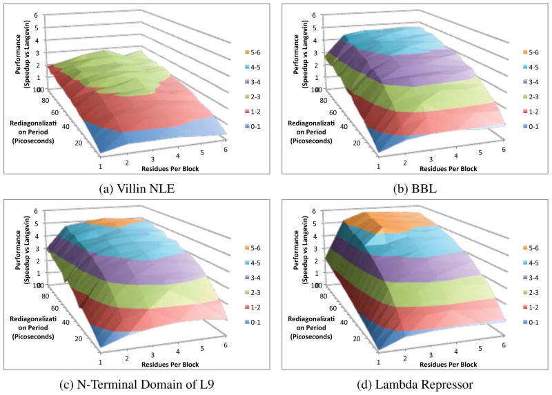
The performance of LTMD is dependent on a number of parameters. The main determinant is how often new eigenvectors are calculated (re-diagonalization of the Hessian). The cost of the eigenvector calculation is, in turn, influenced by the size of the block Hessians (number of residues per block). It was shown that the cost of calculating the eigenvectors was using the Flexible Block Method8 (FBM) with sparse and analytical Hessians. OpenMM LTMD uses numerical differentiation for calculating the block Hessians and quadratic-product matrix S. To quantify the effect of both the period of eigenvector calculation and the number of residues per block, we calculated the speed up (ns per day for LTMD divided by ns per day for OpenMM Langevin) for eigenvector calculation periods in the range of 10 ps to 100 ps and residues per block in the range of 1–6.
OpenMM LTMD’s performance for the four test systems is presented as a function of the number of residues and rediagonalization period in Figure 1. The parameter space has a relatively convex shape which makes the method’s performance easy to optimize and relatively robust to different choices of parameters. Although OpenMM LTMD performance was optimal with 3 residues per block and a rediagonalization period of 100 ps, similar choices of parameters (e.g., 2 or 4 residues per block and rediagonalization periods of 60 ps to 100 ps) provide similar performance.
Figure 1.
A comparison of the performance speed up on four proteins versus OpenMM Langevin for different values of the number of residues per block and the rediagonalization period.
When compared with OpenMM Langevin, speed ups for the smallest model, Villin NLE, were limited to just over two times, while speed ups in excess of 5 times were seen for the larger models (Table 1). LTMD’s absolute performance reached 4.6 μs/day for Villin NLE.
Table 1.
Comparison of relative performance of OpenMM LTMD vs GROMACS on a 6-core CPU and OpenMM Langevin for four protein systems of different sizes.
| Proteins | Speed Up of OpenMM LTMD vs | ||
|---|---|---|---|
|
| |||
| Name | Number of Atoms | OpenMM Langevin | GROMACS |
|
| |||
| Villin NLE | 582 | 2.9× | 38.5× |
| BBL | 707 | 4.8× | 33.6× |
| NTL9 | 881 | 5.2× | 37.9× |
| Lambda Repressor | 1251 | 5.8× | 49.7× |
4.1.2 Comparisons of Relative and Absolute Performance
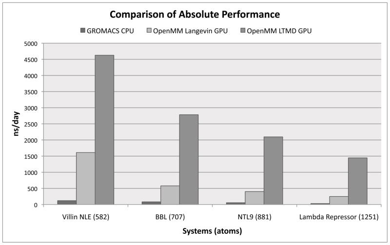
Using the optimal choices for parameters from Section 4.1.1, OpenMM LTMD’s performance was compared to that of OpenMM Langevin and GROMACS with 6 cores. Benchmark simulations were run for each of the four protein systems (Villin NLE, BBL, NTL9, and Lambda Repressor). Absolute performance numbers (given in ns / day) are shown in Figure 2, while relative speed ups were computed and presented in Table 1.
Figure 2.
Comparison of absolute performance (ns/day) between GROMACS with 6 CPU cores, OpenMM Langevin, and OpenMM LTMD.
OpenMM LTMD showed significant increases on absolute performance in comparison with GROMACS and OpenMM Langevin. OpenMM LTMD’s absolute performance peaked at 4.6 μs/day for Villin NLE compared to 0.1 μs/day for GROMACS and 1.6 μs/day for OpenMM Langevin. On larger systems, OpenMM LTMD achieved 2.8 μs/day for BBL, 2.1 μs/day for NTL9, and 1.4 μs/day for Lambda Repressor compared with 0.08 (BBL), 0.06 (NTL9), and 0.03 (Lambda Repressor) μs/day with GROMACS and 0.6 (BBL), 0.4 (NTL9), and 0.2 (Lambda Repressor) μs/day with OpenMM Langevin.
Comparing relative performance (speed up) of OpenMM LTMD over GROMACS and OpenMM Langevin shows that OpenMM LTMD scales better for larger systems versus the other methods. Table 1 details the speed up of OpenMM LTMD over OpenMM Langevin and GROMACS. OpenMM LTMD provides speed ups of up to 5.8× over OpenMM Langevin and 49.7× over GRO-MACS. Of particular interest is that the speed up provided by OpenMM LTMD increases for larger protein systems, implying, along with absolute performance displayed in Figure 2, that OpenMM LTMD scales better than either OpenMM Langevin or GROMACS with system size.
4.1.3 Run-time Breakdown
To provide insight as to where time is being spent, we detailed the steps of the method and profiled the run-time of each step individually. Simulations were run using the optimal parameters choices detailed in Section 4.1.1. The steps are as follows:
Computation of the block Hessians using numerical differentiation of the forces
Diagonalization of the block Hessians
Creation of E by sorting the calculated eigenvalues from the hessian and culling those below a threshold
Computation of HE using numerical differentiation of the forces
Multiplication HE and ET to find S.
Diagonalization of S to find Q
Finding the approximate normal modes U by multiplying E and Q.
The propagation of the system.
Table 2 gives the absolute time for each step in milliseconds for each of the four protein systems, while Figure 3 gives the percent time spent on each step for Villin NLE (our smallest system) and Lambda Repressor (our biggest system). For smaller systems, such as Villin NLE, the run time is dominated by the numerical differentiation of the block Hessians and their diagonalization. Whereas, for larger systems such as Lambda Repressor, run time is dominated by the numerical calculation of S and its diagonalization. The large amount of time spent on diagonalization versus propagation explains why longer rediagonalization periods provide better performance as found in Section 4.1.1.
Table 2.
Run time breakdown for a step of simulation. Time in milliseconds.
| System | Atoms | Comp. Blocks | Diag. Blocks | Calc. E | Calc. HE | Calc. S | Diag. S | Calc. U | Propagate |
|---|---|---|---|---|---|---|---|---|---|
| Villin NLE | 582 | 103.4 | 189.5 | 4.0 | 67.8 | 3.9 | 12.9 | 3.4 | 37.1 |
| BBL | 707 | 135.1 | 325.5 | 6.1 | 121.2 | 6.7 | 22.0 | 7.5 | 62.5 |
| NTL9 | 881 | 122.8 | 224.4 | 11.6 | 200.4 | 10.5 | 51.6 | 13.3 | 85.9 |
| Lambda Repressor | 1251 | 125.0 | 226.7 | 40.6 | 458.3 | 25.7 | 258.6 | 27.3 | 119.7 |
Figure 3.
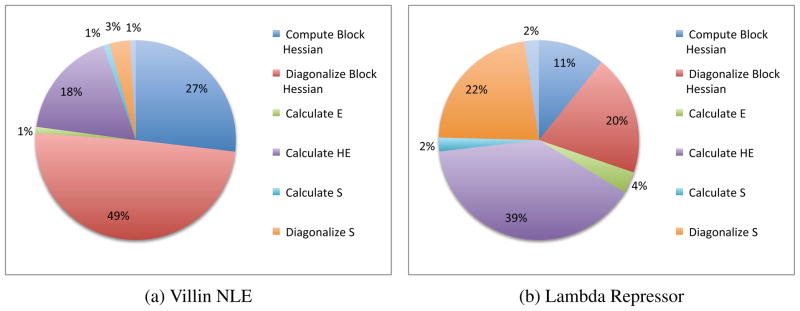
A breakdown of the time spent in each section of the analysis portion of the code for the smallest (Villin NLE) and largest (Lambda Repressor) systems tested.
4.2 Validation
OpenMM LTMD was validated against OpenMM Langevin through simulations of Ala5,37 a small peptide of five alanines, and Villin NLE, a variant of the Villin headpiece that folds in 0.5 μs.
4.2.1 Dynamics and Sampling of the Small, Helical Peptide Ala5
Ala5 was simulated with OpenMM LTMD and Langevin to validate that LTMD properly reproduces dynamics and sampling. The Ala5 model was prepared with the Amber96 forcefield and the Generalized Born OBC implicit-solvent model. Eighteen simulations for both Langevin and LTMD, with total aggregate times of 5.4 μs and 4.8 μs each, were run from an extended confirmation at 300 °K. The LTMD simulations used the following choice of parameters: 16 modes, 5 fs timestep, 625 fs rediagonalization period, 1 residue per block, 18 vectors per block, a block epsilon of 1 × 10⁻⁵ Å, and an s epsilon of 1 × 10⁻⁴ Å. The folded “helical” state for each alanine residue was defined by having φ and ψ angles such that −180° ≤ φ ≤ 0° and −120° ≤ ψ ≤ 15°.37
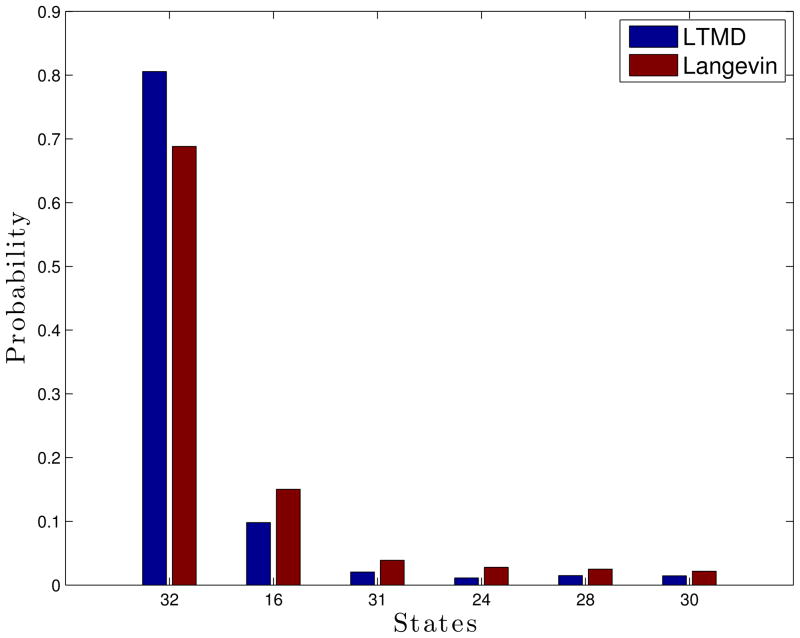
To compare sampling accuracy we measured the state distributions, where the states of the individual residues are deemed folded or unfolded by the criterion defined above. Ala5 has 32 states defined by the permutation of folded and unfolded states for each of its five residues. A comparison of the state distributions from the LTMD and Langevin simulations shows that LTMD samples the states with similar probability as Langevin, indicated by a correlation of 0.99 (Figure 4). Both methods show Ala5 spending most of its time in state 32 (all of the residues are folded), with the majority of the remaining time in state 16 (one of the end residues is unfolded). LTMD has a lower probability of being in state 16 and a higher probability of being in state 32.
Figure 4.
Populations of the 6 most-populated of the 32 defined states of Ala5 from Ala5 Amber96, GB-OBC implicit-solvent simulations run with LTMD (blue) and Langevin (red). All simulations started from an extended structure.
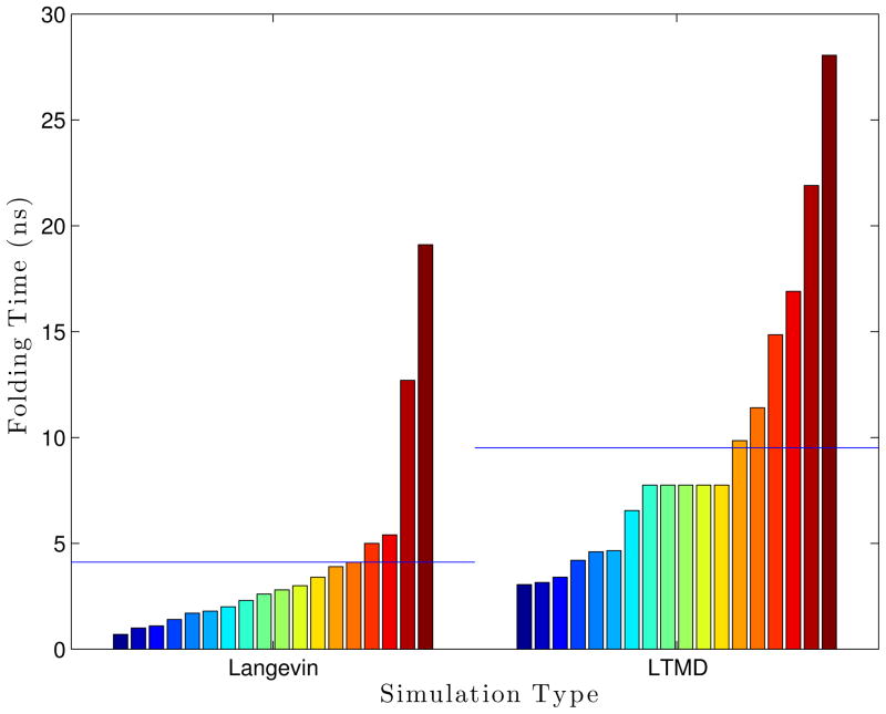
To compare the dynamics we define the folded state of the peptide by all three inner alanine residues being folded, as defined above. We observed the time for each of the simulations to reach this folded state, from its initial extended state. The mean first passage folding time for the Langevin simulations was 4.1 ns with a standard deviation of 4.6 ns. The LTMD Ala5 simulations produced mean folding times of 9.5 ns with a standard deviation of 6.9 ns, which within the error is comparable to the Langevin simulations.
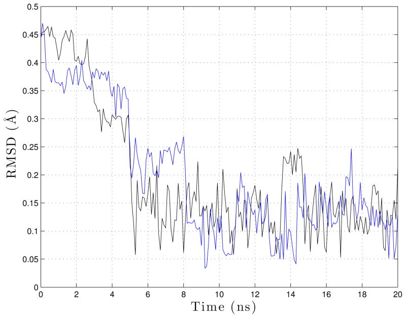
To measure the dynamics qualitatively we consider the RMSD, relative to the folded helical structure, during the folding process RMSD was computed for one representative Langevin simulation (black) and one representative LTMD simulation (blue) (Figure 6). Both simulations folded in 5.0 ns. The RMSD plots for both simulations show similar collapses at 5.0 ns as well as subsequent folding and unfolding.
Figure 6.
RMSD against the folded structure was computed for Langevin (black) and LTMD (blue).
4.2.2 Folding of Villin NLE
Villin NLE simulations were run with LTMD and OpenMM Langevin to validate the correctness of the LTMD implementation over longer timescales. The Villin NLE model was prepared with the Amber99-SB forcefield and the Generalized Born OBC implicit-solvent model. The dynamics of the simulations were analyzed with respect to their ability to fold Villin NLE. It should be noted that our emphasis is purely on validating the correctness of the LTMD implementation, not on a large-scale analysis of Villin NLE dynamics.
Figure 7 gives the RMSD plots for two representative LTMD simulations run at 370 °K with a 50 fs timestep, 10 modes, and a rediagonalization period of 25 ps. The RMSDs were calculated against the native structure using the Cα atoms, excluding the first and last two residues. The first simulation (Figure 7a) folds Villin NLE to within 3.6Å of the native structure, where it remains for around 1 μs. In the second simulation (Figure 7b), the protein undergoes multiple folding and unfolding events, occurring approximately every 0.5 μs, and is able to fold to within 3.5 Å of the native structure. While Langevin simulations fold Villin NLE to within 3 Å of the native structure, it should be noted that the higher RMSD of the LTMD simulations is an expected result given the coarse-graining used by the method to obtain better performance. As evidenced by these two simulations, LTMD is able to capture the dynamics of the proteins, while enabling a significant speed up over traditional MD.
Figure 7.
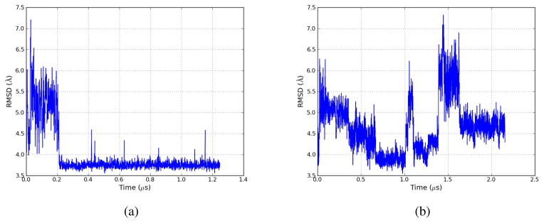
RMSD plots for two Villin NLE Amber99-SB, GB-OBC implicit-solvent simulations run with LTMD. RMSD was calculated using Cα atoms, excluding the first two and last two residues, against the folded structure. The minimum RMSDs of each simulation are 3.6 Å and 3.5 Å, respectively. Figure 7b shows multiple folding and unfolding events, occurring approximately every 0.5 μs.
4.3 Parameter Choices and Diagnostics
OpenMM LTMD uses multiple user supplied parameters in order to propagate and diagonalize the system of interest. In Section 4.3.1 the effect of varying the rate of rediagonalization on the dynamics is measured and in Section 4.3.2 the effects of the number of modes used on the dynamics is measured. We look at the effect of parameters on the accuracy of FBM in Sections 4.3.3 – 4.3.5. Section 4.3.3 compares the FBM implementation in OpenMM against the reference implementation in ProtoMol and the approximate eigenvectors with the full eigenvectors. In Section 4.3.4 the effect of the epsilons, ε, used as the perturbation for the numerical differentiation operations required within FBM. In Section 4.3.5 the effects of different partitioning schemes within FBM are compared. In Section 4.3.6 we consider the effects of the “noise” term in the Euler-Maruyama approximation in the fast space.
4.3.1 Rediagonalization Period
The theory behind LTMD assumes that the modes are always valid which, in theory, would require diagonalization at every step. In practice it has been observed that, since we only use a few low frequency modes, this requirement can be relaxed.
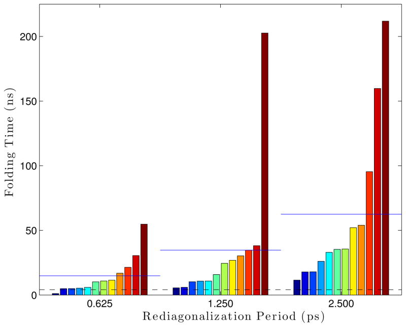
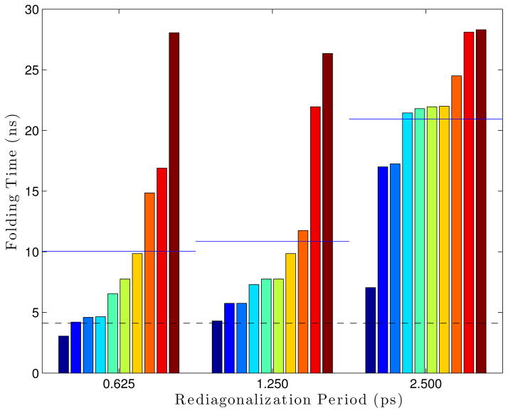
The effect of the rediagonalization period on the folding rate was measured by running Ala5 simulations with different rediagonalization periods (0.625 ps, 1.25 ps, and 2.5 ps) for 300 ns with parameters: 300 °K, 5 fs timestep, 12 modes, 1 residue per block, 14 vectors per block, and epsilons of 1 × 10⁻⁴ Å for the S matrix and 1 × 10⁻⁵ Å for the blocks. Rediagonalization period proved to affect the folding rate significantly. Simulations run with a rediagonalization period of 2.5 ps folded in an average of 62.5 ns, much larger than the average folding time of 3.7 ns found from Langevin simulations. Decreasing the rediagonalization period to 0.625 ps reduced the average folding time to 14.3 ns.
This test was repeated, using 16 modes instead of 12 (which was found to be more accurate in Section 4.3.2). Here, we see that simulations run with a rediagonalization period of 2.5 ps had an average folding time of 20.94 ns. When the period is dropped to 1.25 ps or 0.625 ps, the average folding time drops to around 10 ns. This seems to indicate that picking the best number of modes to run, could allow a larger rediagonalization period before losing accuracy, allowing a trade-off to optimize performance.
4.3.2 Number of Modes
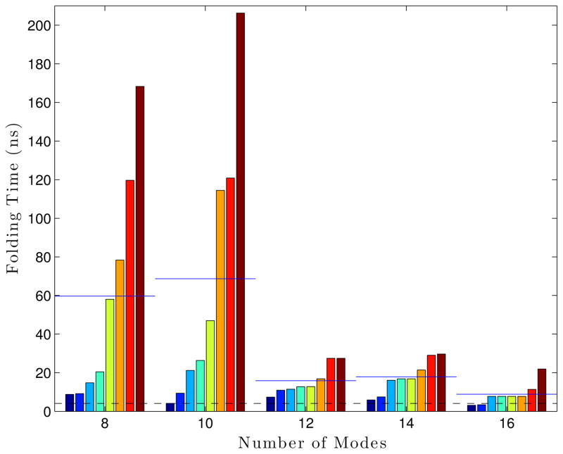
A sweep of the number of modes was performed. Eight Ala5 LTMD simulations were run for each mode setting (8, 10, 12, 14, and 16 modes) for 300 ns at 300 °K, 5 fs timestep, 1 residue per block, and epsilons of 1×10⁻⁵ Å for the blocks and 1×10⁻⁴ Å for the S matrix. The number of vectors per block was set to be number of modes plus two (10, 12, 14, 16, and 18 vectors per block, respectively). With 16 modes, the LTMD Ala5 simulations were able to consistently achieve folding times of 5.5 ns on average with a standard deviation of 2.6 ns, which compares favorably to the values obtained from Langevin simulations (average of 3.7 ns and standard deviation of 3.9 ns).
4.3.3 Approximate Eigenvector Overlap
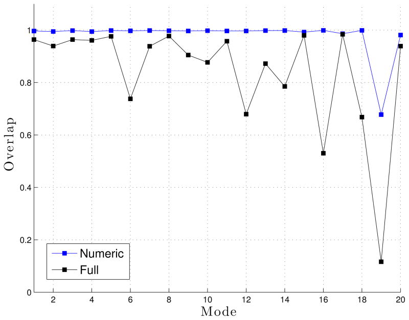
The implementation of the Flexible Block Method (FBM) in LTMD was validated against the implementation in ProtoMol using a metric called “overlap.” Overlap (as described in Tama, et al.26) measures how well a vector is represented by a space spanned by a set of vectors. The overlap Pj for a reference eigenvector uj with the set of approximate eigenvectors (v1, v2, …vm) is given by Eq. (16). An overlap value of 1 indicates that the reference eigenvector is represented completely by the approximate eigenvectors, while a value of 0 means that the reference eigenvectors is not represented at all.
| (16) |
We used overlap to compare the approximate eigenvectors generated from both the reference CPU Flexible Block Method (FBM) implementation in ProtoMol38 and our implementation in LTMD. Figure 11 shows the overlap for the approximate eigenvectors from LTMD with those produced by the FBM implemented in ProtoMol in WW Fip35. The two implementations show very good agreement for the first 20 modes. We also computed the overlap between the approximate eigenvectors from LTMD with the full eigenvectors. The approximate eigenvectors agree with the full eigenvectors for the first 15 modes but are less accurate for modes 16, 18, and 19. Since only ten or twelve modes are used in simulations, FBM is able to approximate the eigenvectors reasonably well for our purposes.
Figure 11.
Overlap between the approximate eigenvectors forWWFip35 for LTMD and ProtoMol implementations of FBM (blue) and the approximate eigenvectors and full eigenvectors (black).
4.3.4 Magnitude of Epsilon for Numerical Differentiation Perturbation
As detailed in the Section 2.2, LTMD uses the Flexible Block Method (FBM) to perform a fast normal mode analysis which utilizes numerical differentiation (ND). The choice of perturbation ε is usually made to be as small as possible so that accuracy is maintained, while being large enough to avoid round-off errors due to the finite precision of floating-point arithmetic. For single precision arithmetic, an optimal value for ε can generally be found as .39 Note that OpenMM LTMD uses units of nm internally; for our configuration files this equates to ε = 3.4 × 10⁻⁵ Å. For FBM there are additional considerations when finding the ε for the formation of the S matrix since it is important that our perturbation lies in the low frequency space of interest. Since, when projected from mode space our perturbation vector, δm, is given by for the ith mode, all of the values in δm must not have significant round-off. Below, we document the tests carried out to determine the optimal values for the ε used in the block and S matrix ND and compare to theory.
From Langevin simulations, it is known that the extended confirmation of WW-Fip35 rapidly collapses. We have found that LTMD simulations of the collapse are particularly sensitive to the choice of εs and thus are an excellent test for validation.
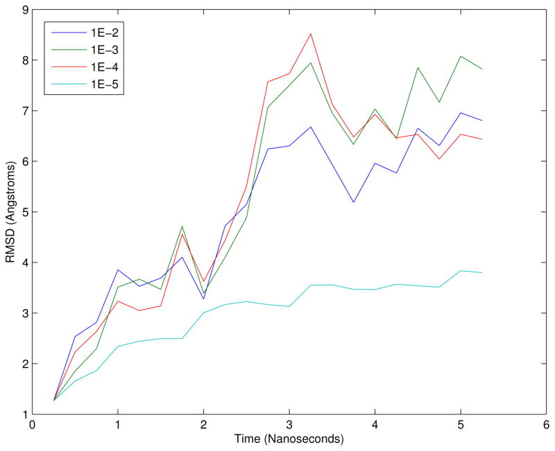
To measure the effect of the choice of ε on the dynamics, WW-Fip35 was simulated from an extended confirmation with a range of values for ε. The WW-Fip35 model was prepared from the extended confirmation using the Amber96 forcefield and Generalized Born OBC implicit-solvent model. LTMD simulations were run with a 50 fs timestep, 10 modes, a 100 ps rediagonalization period, and a range of values for ε. RMSD to the extended structure was calculated between the Cα atoms and plotted as a function of time in Figure 12. Simulations run with values between 1 × 10⁻² Å and 1 × 10⁻⁴ Å show similar rates of collapse, while the simulation with ε = 1 × 10⁻⁵ Å shows that the dynamics are damped and the protein is prevented from collapsing.
Figure 12.
Comparison of the collapse of WW-Fip35 from the extended confirmation with different magnitudes for the numerical differentiation perturbations. RMSD was computed against the extended confirmation. The other simulations were run with LTMD using different values of ε. The same choice of ε was used for both the blocks and quadratic product.
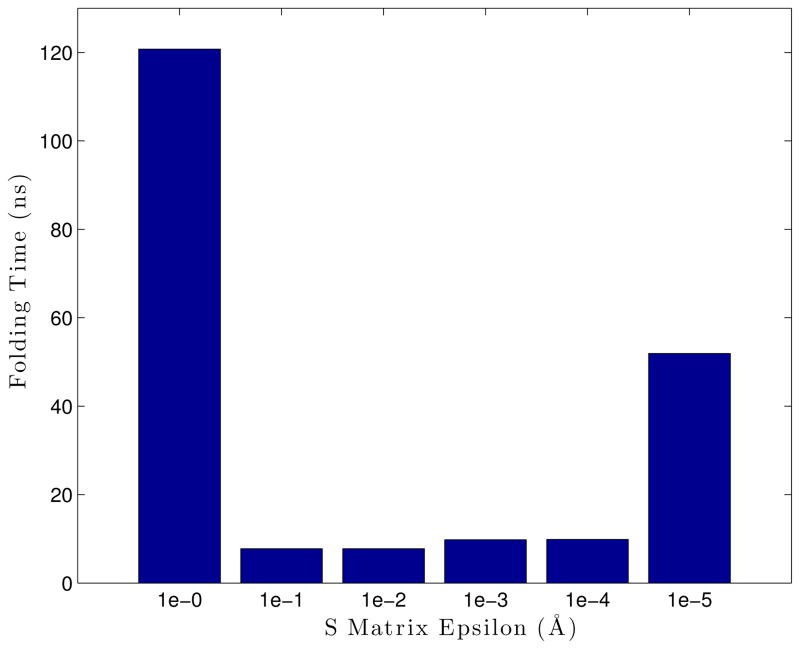
To further explore the effects of the S matrix epsilon on the simulation folding time, a sweep of simulations were run with varying S matrix epsilons using Ala5. In Figure 13, we can see that this epsilon value should not be a critical factor in simulation accuracy (at least for the Ala5 model), beyond being within the right range.
Figure 13.
A sweep of simulations executed with varying S matrix epsilons, with the Ala5 model. Each bar is a single simulation, where all bars within a group all use the same parameters. The groups are sorted within themselves. The blue lines drawn over each set of bars are the average folding time for that set, while the dashed black line gives the “reference” folding time from Langevin simulations.
4.3.5 Effect of Partitioning Method
The Flexible Block Method (FBM) requires choosing a method for partitioning the atoms into blocks.26–30 The simulations in this paper, group entire residues into blocks using a uniform number of residues per block (the last block may contain fewer if the number of residues is not an integer multiple of the number of residues per block). To look at the effect of the partitioning, an alternative scheme was devised where the partitioning occurs after the Cα atoms along the backbone. The atoms in the blocks for both partitioning methods represent a sequential set.
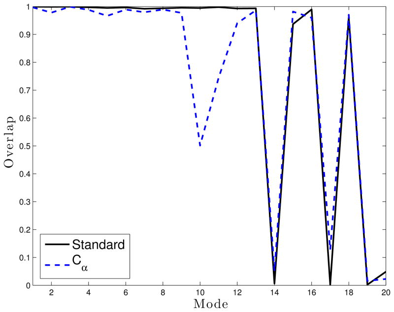
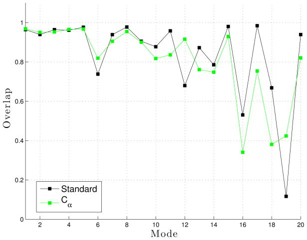
The two schemes were compared with respect to the overlaps of the first 20 approximate eigenvectors against the first 20 real eigenvectors (Figure 14) and folding time of Ala5 LTMD simulations. The eigenvectors were calculated using 1 residue per block, 18 vectors per block, and epsilons of 1×10⁻⁵ Å for the blocks and 1×10⁻⁴ Å for the S matrix. The standard partitioning scheme reproduces the first 11 modes very well but is not able to reproduce modes 14, 17, or 19. The Cα partitioning scheme has similar accuracy for all modes except for modes 10–12, which it is not able to reproduce well. Reflecting the difference in the accuracy of the modes with the two partitioning schemes, a LTMD simulation with the standard partitioning scheme folded Ala5 in 24.8 ns, more quickly than a simulation with the Cα partitioning scheme at 33.7 ns.
Figure 14.
Overlap for Residue (standard) and Cα partitioning schemes for Ala5 compared with modes from a “brute force” diagonalization.
The two schemes were also tested onWWFip35 (Figure 15). The accuracy of the two schemes is similar, suggesting that the two schemes do not make a significant differnece in the accuracy of the modes.
Figure 15.
Overlap for Residue (standard) and Cα partitioning schemes for WW Fip35 compared with modes from a “brute force” diagonalization.
4.3.6 Magnitude of Fast Noise
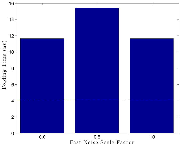
As an approximation to Euler-Murayama method, after performing minimization in the fast space LTMD adds random noise Eq. (5). Ala5, with different amounts of fast noise, was simulated to measure the effect of the noise on dynamics (Figure 16). The simulations were run for 300 ns with the following parameters: 300 °K, 5 fs timestep, 16 modes, a rediagonalization period of 0.625 ps, 1 residue per block, 18 vectors per block, and epsilons of 1×10⁻⁵ Å for the blocks and 1×10⁻⁴ Å for the S matrix. The figure shows that the noise factor, for this model, did not have a great effect. However, from these results, a noise scaling value of 1.0 allows for the closest average folding time compared to the Langevin tests.
Figure 16.
Folding times of LTMD Ala5 simulations run with different values for the amount of noise added in the fast space. Each bar is an average computed from four simulations. The dashed black line gives the “reference” folding time from Langevin simulations.
5 Conclusions and Future Work
We have presented a hybrid CPU/GPU implementation of the LTMD propagator with speed ups of over 5.8× compared with traditional MD integrators on GPUs. This result illustrates great potential for testing larger protein systems over a longer biological period of time. Analysis of the cost of individual sections of the method have yielded insight into how we may improve performance in the future.
Validation with Ala5 and Villin NLE has shown excellent agreement between Langevin and LTMD. With Ala5, we showed that LTMD is able to sample the conformational states with a similar distribution as Langevin, produces comparable folding times, and captures similar dynamics. Similar folding times and dynamics between Langevin and LTMD were also reported for Villin NLE.
Analyses of the effects of the various parameters such as rediagonalization period, the number of modes, epsilons used with the numerical differentiation, partitioning methods, and fast noise were presented. We found that with the proper parameters, especially the rediagonalization period and number of modes, LTMD agrees well with Langevin. Further, by choosing a larger number of modes, rediagonalization can be performed less frequently, leading to increased performance. The choice of block epsilons for FBM were shown to agree with the known values from the theory, while the choice of S epsilons were shown to be robust over a range of values.
We would like to move the entire algorithm to the GPU eventually. CPU portions of the algorithm currently include block diagonalization, diagonalization of S and numerical differentiation. We anticipate that porting this code to the GPU should help reduce data transfers between the two processors and take advantage of the GPU’s ability to parallelize operation, which will improve performance. Given that the diagonalization dominates the run-time of the method, performance improvements can lead to even greater gains in raw simulation performance (e.g., ns/day).
The code for LTMD is part of OpenMM and will be released as a plugin. This implementation of LTMD, and future improvements to the performance and numerics promise an order of magnitude improvement over conventional GPU implementations of MD. We are working on multilevel FBM methods, which should scale as O(N logN) and thus enable even larger system simulations, and on extensions of LTMD to explicit solvent systems. These will be reported in future papers.
Figure 5.
Folding times of Ala5 Amber96, GB-OBC implicit-solvent simulations run with Langevin and LTMD. The blue lines give the average folding times for each simulation method. Eighteen simulations of each type were run, and all simulations started from an extended structure.
Figure 8.
Rediagonalization period’s effect on the folding time using 12 modes. Each bar is a single simulation, where all bars within a group all use the same parameters. The groups are sorted within themselves. The blue lines drawn over each set of bars are the average folding time for that set, while the dashed black line gives the “reference” folding time from Langevin simulations.
Figure 9.
Rediagonalization period’s effect on the folding time using 16 modes. Each bar is a single simulation, where all bars within a group all use the same parameters. The groups are sorted within themselves. The blue lines drawn over each set of bars are the average folding time for that set, while the dashed black line gives the “reference” folding time from Langevin simulations.
Figure 10.
The effect on the folding time, caused by changing the number of modes. Each bar is a single simulation, where all bars within a group all use the same parameters. The groups are sorted within themselves. The blue lines drawn over each set of bars are the average folding time for that set, while the dashed black line gives the “reference” folding time from Langevin simulations.
Acknowledgments
JAI, CRS and VSP acknowledge funding from NIH 1R01GM101935-01. JAI and CRS also acknowledge funding from NSF CCF 1018570. RJN was supported by an OpenMM Visiting Scholar Fellowship in the summer of 2012. TMC acknowledges funding from a Faculty Development Grant from Eckerd College. We acknowledge the use of a GPU cluster at the Center for Research Computing at University of Notre Dame for development and validation. We acknowledge the use of a GPU cluster at the Institute for Computational and Mathematical Engineering (ICME) at Stanford University for validation. We would like to thank Dr. Peter Eastman for helpful discussions and advice. JAI gratefully acknowledges Jeff Peng’s introduction to the NMR dynamics of the WW domain.
A Source Code
Listing 1. Projection Kernel.
void Projection Kernel (int atoms , int modes , float4 * vel , float4 *mode , float *mode_weight) {
  extern _ _shared _ _float buffer [ ] ;
  for ( int mode = blockIdx . x ; mode < modes ; mode += gridDim . x ) {
   Real dot = 0.0f;
   for (int atom = threadIdx . x; atom < atoms; atom += blockDim . x ) {
     const int modePos = mode * atoms + atom ;
     const Real scale = 1. 0 f / sqrt ( vel [atom] . w ) ;
     float4 v = vel [atom] ;
     float4 m = mode [modePos] ;
     dot += scale * ( v . x * m . x + v . y * m . y + v . z * m . z ) ;
   }
   buffer[ threadIdx . x] = dot ;
   _ _ syncthreads ( ) ;
   if ( threadIdx . x == 0 ) {
     Real sum = 0 ;
     for ( int i = 0 ; i < blockDim . x ; i++ ) {
       sum += buffer [ i ] ;
     }
     mode_weight [mode ] = sum;
   }
  }
}
A.1 Diagonalization with Flexible Block Method
A.1.1 Computation of Block Hessian
Listing 2. Computation of Hessian.
/ / Create copies of the current state
. . .
/ / Set positions to initial state
. . .
/ / Calculate perturbation of the ith degree of freedom in EACH block
TNT : : Array2D<double > h ( n, n, 0.0 ) ;
for ( int i = 0 ; i < LargestBlockSize ; i ++) {
  / / Calculate perturbed positions
  for ( int j = 0 ; j < blocks . size ( ) ; j ++) {
   const int DOF = 3 * blocks [ j ] + i ;
   const int atom = DOF / 3 ;
   / / Cases to not perturb, in this case just skip the block
   if ( j == blocks . size ( ) – 1 && atom >= ParticleCount) continue ;
   if ( j != blocks . size ( ) – 1 && atom >= blocks [ j + 1 ] ) continue ;
   Backward [ atom ] [DOF%3] = Initial [ atom ] [DOF%3] – Delta ;
   Forward [ atom ] [DOF%3] = Initial [ atom ] [DOF%3] + Delta ;
  }
  / / Using the GPU Calculate backwards perturbation
  . . .
  / / Using the GPU Calculate forwards perturbation
  . . .
  / / Revert forward and backward block positions to initial state
  . . .
  / / Fill Matrix
  for (int j = 0 ; j < blocks . size ( ) ; j ++) {
   const int DOF = 3 * blocks [ j ] + i ;
   const int atom = DOF / 3 ;
   / / Cases to not perturb, in this case just skip the block
   if ( j == blocks . size ( ) – 1 && atom >= ParticleCount ) continue ;
   if ( j != blocks . size ( ) – 1 && atom >= blocks [ j +1 ] ) continue ;
   const int col = DOF;
   const int start_dof = 3 * blocks [ j ] ;
   const int end_dof = ( j == blocks . size ( ) – 1) ? 3 * ParticleCount : 3 *
      blocks [ j + 1 ] ;
   for ( int k = start_dof ; k < end_dof ; k++) {
     double blockscale = 1.0 / (2 * Delta * sqrt ( ParticleMass [ atom ] *
        ParticleMass [ k / 3 ] ) ) ;
     h [ k ] [ col ] = ( forces 1 [ k / 3 ] [ k % 3] – forces 2 [ k / 3 ] [ k%3]) * blockscale ;}
   }
  }
}
We show our steps for computing the block Hessian matrices in Listing 2. Matrix h is an n × n matrix initialized to zeroes which will hold the block Hessian matrices on the diagonal. Each block will be a square matrix which accounts for a certain number of degrees of freedom, the largest of which is stored in LargestBlockSize. We initialized blocks[j] to have the starting index of the jth block, thus the ith degree of freedom of block j becomes 3*blocks[j]+i. We perturb this degree of freedom in both the forward and backward direction by some small Delta value, then use the GPU to calculate forces in both directions which we store in forces1 and forces2, respectively. Note that we must check to make sure that blocks[j]+i falls within block j, otherwise we must discard this degree of freedom. This is necessary because not all blocks will have a size of LargestBlockSize.
We then populate the appropriate entries of the block Hessian matrices by using the second j loop. Once again, the degree of freedom (DOF) becomes equal to 3*blocks[j]+i, which is the same as the column in the h matrix. The k loop counts over the starting and ending degrees of freedom for block j, and we approximate the second derivative of the positions using second-order finite difference with the forward and backward perturbed forces. Note the entries are mass-reweighted.
A.1.2 Computation of S
Listing 3. Computation of S and HE.
/ / Create matrix structures
. . .
/ / Store a temporary copy of the positions
. . .
/ / Loop over all columns of the matrix
for ( int k = 0 ; k < m; k++) {
  / / Calculate forward perterbation
  for ( int i = 0 ; i < ParticleCount ; i ++) {
   for ( int j = 0 ; j < 3 ; j ++) {
     const double RootMass = sqrt ( ParticleMass [ i ] ) ;
     Temporary [ i ] [ j ] = Positions [ i ] [ j ]+ eps *E[3* i + j ] [ k ] / RootMass ;
   }
  }
  / / Using the GPU calculate forward force
  . . .
  / / Calculate backward perturbations
  . . .
  / / Using the GPU calculate backward force
  . . .
  / / Create HE from the perterbed forces
  for ( int i = 0 ; i < n ; i ++) {
   const double ScaleFactor = sqrt ( ParticleMass [ i / 3 ] ) *2. 0* eps ;
   HE[ i ] [ k ] = ( Forward [ i / 3 ] [ i%3]–Backward [ i / 3 ] [ i %3]) / ScaleFactor ;
  }
  / / Restore positions
  . . .
}
We show our computation of S in Listing 3. After saving our current atomic position vector, we perturb atom i’s position by a value of ε times E multiplied by the square root of the atomic mass of particle i. We then calculate the force vector using the perturbed positions on the GPU by invoking the OpenMM API which is responsible for distributing molecular force calculations across GPUs by calling routines from CUDA. Upon completion, the GPU code sends the force vector back which we store in an array Forward.
We follow our forward perturbed force calculation with an analogous backward perturbation of positions, this time by −εEiM−1/2. We then calculate the force vector using the backward perturbed positions on the GPU and store the result in an array Backward, similar to before. Upon dividing the difference between Forward and Backward by 2ε, we complete our calculation of , the ith column of ETH. Once we have done this for all DOF we multiply by to get S.
Footnotes
6 Availability
The implementation reported in this manuscript will be made available on Github (https://github.com/LCLS/LTMDOpenMM) as a plugin for OpenMM.
References
- 1.Izaguirre JA, Skeel RD. Computational Molecular Dynamics: Challenges, Methods, Ideas, Vol. 4 of Lecture Notes in Computational Science & Engineering. Springer-Verlag; Berlin: 1998. pp. 303–318. [Google Scholar]
- 2.Ma Q, Izaguirre JA, Skeel RD. SIAM J Sci Comput. 2003;24:1951–1973. [Google Scholar]
- 3.Schlick T. Molecular Modeling and Simulation. Springer-Verlag; New York: 2002. [Google Scholar]
- 4.Shirts M, Pande VS. Science. 2000;290:1903–1904. doi: 10.1126/science.290.5498.1903. [DOI] [PubMed] [Google Scholar]
- 5.Beberg AL, Ensign DL, Jayachandran G, Khaliq S, Pande VS. 2009 IEEE International Symposium on Parallel & Distributed Processing; 2009. pp. 1–8. [Google Scholar]
- 6.Izaguirre JA, Catarello DP, Wozniak JM, Skeel RD. J Chem Phys. 2001:114. [Google Scholar]
- 7.Sweet CR, Petrone P, Pande VS, Izaguirre JA. J Chem Phys. 2008;128:145101. doi: 10.1063/1.2883966. [DOI] [PMC free article] [PubMed] [Google Scholar]
- 8.Izaguirre JA, Sweet CR, Pande VS. Multiscale Dynamics of Macromolecules Using Normal Mode Langevin. 2010 doi: 10.1142/9789814295291_0026. http://dblp.uni-trier.de/db/conf/psb/psb2010.html#IzaguirreSP10. [DOI] [PMC free article] [PubMed]
- 9.Deutch JM, Oppenheim I. J Chem Phys. 1971;54:3547. [Google Scholar]
- 10.Shaw DE, Chao JC, Eastwood MP, Gagliardo J, Grossman JP, Ho CR, Ierardi DJ, Kolossváry I, Klepeis JL, Layman T, McLeavey C, Deneroff MM, Moraes Ma, Mueller R, Priest EC, Shan Y, Spengler J, Theobald M, Towles B, Wang SC, Dror RO, Kuskin JS, Larson RH, Salmon JK, Young C, Batson B, Bowers KJ. ACM SIGARCH Computer Architecture News. 2007;35:1. [Google Scholar]
- 11.Shaw D, Deneroff M, Dror R, Kuskin J, Larson R, Salmon J, Young C, Batson B, Bowers K, Chao J, et al. Communications of the ACM. 2008;35:91–97. [Google Scholar]
- 12.Shaw D, Dror R, Salmon J, Grossman J, Mackenzie K, Bank J, Young C, Deneroff M, Batson B, Bowers K, et al. Millisecond-scale molecular dynamics simulations on Anton. 2009 http://portal.acm.org/citation.cfm?id=1654126.
- 13.Shaw DE, Maragakis P, Lindorff-Larsen K, Piana S, Dror RO, Eastwood MP, Bank Ja, Jumper JM, Salmon JK, Shan Y, Wriggers W. Science. 2010;330:341–346. doi: 10.1126/science.1187409. [DOI] [PubMed] [Google Scholar]
- 14.Stone JE, Hardy DJ, Ufimtsev IS, Schulten K. J Mol Graphics. 2010;29:116–125. doi: 10.1016/j.jmgm.2010.06.010. [DOI] [PMC free article] [PubMed] [Google Scholar]
- 15.Stone JE, Phillips JC, Freddolino PL, Hardy DJ, Trabuco LG, Schulten K. J Comp Chem. 2007;18:2618–40. doi: 10.1002/jcc.20829. [DOI] [PubMed] [Google Scholar]
- 16.Phillips JC, Stone JE, Schulten K. Adapting a Message-Driven Parallel Application to GPU-Accelerated Clusters. 2008. [Google Scholar]
- 17.Onufriey A, Bashford D, Case DA. J Comp Chem. 2002;23:1297–1304. doi: 10.1002/jcc.10126. [DOI] [PubMed] [Google Scholar]
- 18.Phillips C, Stone JE, Schulten K. Adapting a message driven parallel application to GPU-accelerated clusters. 2008. [Google Scholar]
- 19.Darden T, York D, Pederson L. J Chem Phys. 1993;98:10089–10092. [Google Scholar]
- 20.Gotz AW, Williamson MJ, Xu D, Poole D, LeGrand S, Walker RC. J Chem Theory Comput. 2012;8:1542–1555. doi: 10.1021/ct200909j. [DOI] [PMC free article] [PubMed] [Google Scholar]
- 21.Harvey MJ, Giupponi G, Fabritiis GD. J Chem Theory Comput. 2009;5:1632–1639. doi: 10.1021/ct9000685. [DOI] [PubMed] [Google Scholar]
- 22.Friedrichs M, Eastman P, Vaidyanathan V, Houston M, Legrand S, Beberg A, Ensign D, Bruns C, Pande V. J Comp Chem. 2009;30:864–872. doi: 10.1002/jcc.21209. [DOI] [PMC free article] [PubMed] [Google Scholar]
- 23.Eastman P, Pande VS. Comput Sci Eng. 2010;12:34–39. doi: 10.1109/MCSE.2010.27. [DOI] [PMC free article] [PubMed] [Google Scholar]
- 24.Ewald PP. Ann Phys. 1921;369:253–287. [Google Scholar]
- 25.Durand P, Trinquier G, Sanejouand Y. Biopolymers. 1994;34:759–771. [Google Scholar]
- 26.Tama F, Gadea FX, Marques O, Sanejouand YH. PROTEINS: Struc, Func, and Genetics. 2000;41:1–7. doi: 10.1002/1097-0134(20001001)41:1<1::aid-prot10>3.0.co;2-p. [DOI] [PubMed] [Google Scholar]
- 27.Ghysels A, Van Neck D, Van Speybroeck V, Verstraelen T, Waroquier M. J Chem Phys. 2007:126. doi: 10.1063/1.2737444. [DOI] [PubMed] [Google Scholar]
- 28.Ghysels A, Van Neck D, Waroquier M. J Chem Phys. 2007:127. doi: 10.1063/1.2789429. [DOI] [PubMed] [Google Scholar]
- 29.Ghysels A, Van Neck D, Brooks BR, Van Speybroeck V, Waroquier M. J Chem Phys. 2009:130. doi: 10.1063/1.3071261. [DOI] [PMC free article] [PubMed] [Google Scholar]
- 30.Ghysels A, Van Speybroeck V, Pauwels E, Van Neck D, Brooks BR, Waroquier M. J Chem Theory Comput. 2009;5:1203–1215. doi: 10.1021/ct800489r. [DOI] [PubMed] [Google Scholar]
- 31.Kolossváry I, McMartin C. J Math Chem. 1992;9:359–367. [Google Scholar]
- 32.Goldstone J, Salam A, Weinberg S. Phys Rev. 1962;127:965–970. [Google Scholar]
- 33.Folwer M. Patterns of Enterprise Application Architecture. Addison-Wesley; Boston: 2002. [Google Scholar]
- 34.Intel. The Math Kernel Library; 2012. http://software.intel.com/en-us/articles/intel-mkl/ [Google Scholar]
- 35.OpenCL. The Open Standard For Parallel Programming of Heterogeneous Systems. 2012 http://www.kronos.org/opencl/
- 36.Dagum L, Menon R. IEEE Computational Science & Eng. 1998;5:46–55. [Google Scholar]
- 37.Buchete NV, Hummer G. The Journal of Physical Chemistry B. 2008;112:6057–69. doi: 10.1021/jp0761665. [DOI] [PubMed] [Google Scholar]
- 38.Matthey T, Cickovski T, Hampton S, Ko A, Ma Q, Nyerges M, Raeder T, Slabach T, Izaguirre JA. ACM Trans Math Soft. 2004;30:237–265. [Google Scholar]
- 39.Press WH, Teukolsky SA, Vetteringly WT, Flannery BP. Numerical Recipes in C++ Cambridge; New York: 2002. [Google Scholar]


