

Summary
The ability to focus on and understand one talker in a noisy social environment is a critical social-cognitive capacity, whose underlying neuronal mechanisms are unclear. We investigated the manner in which speech streams are represented in brain activity and the way that selective attention governs the brain’s representation of speech using a ‘Cocktail Party’ Paradigm, coupled with direct recordings from the cortical surface in surgical epilepsy patients. We find that brain activity dynamically tracks speech streams using both low frequency phase and high frequency amplitude fluctuations, and that optimal encoding likely combines the two. In and near low level auditory cortices, attention ‘modulates’ the representation by enhancing cortical tracking of attended speech streams, but ignored speech remains represented. In higher order regions, the representation appears to become more ‘selective,’ in that there is no detectable tracking of ignored speech. This selectivity itself seems to sharpen as a sentence unfolds.
Introduction
The Cocktail Party effect (Cherry, 1953) elegantly illustrates humans’ ability to ‘tune in’ to one conversation in a noisy scene. Selective attention must play a role in this essential cognitive capacity; nonetheless the precise neuronal mechanisms are unclear. Recent studies indicate that brain activity preferentially tracks attended relative to ignored speech streams, using both the phase of low frequency neural activity (1-7 Hz) (Ding and Simon, 2012a, b; Kerlin et al., 2010) and the power of high gamma power activity (70-150 Hz) (Mesgarani and Chang, 2012). Low-frequency activity is of interest because it corresponds to the time scale of fluctuations in the speech envelope (Greenberg and Ainsworth, 2006; Rosen, 1992), which is crucial for intelligibility (Shannon et al., 1995). High gamma power is of interest because it is thought to index the mass firing of neuronal ensembles (i.e., multiunit activity, MUA; Kayser et al., 2007; Nir et al., 2007), thus linking speech tracking more directly to neuronal processing (Mesgarani and Chang, 2012; Pasley et al., 2012). Because the low frequency field potentials measured by electrocorticography (ECoG) reflect the synaptic activity that underpins neuronal firing (Buzsaki, 2006), there is likely to be a mechanistic relationship between these two speech tracking indices (Ghitza, 2011; Giraud and Poeppel, 2012; Nourski et al., 2009), however, the details are not well understood.
Prior studies reporting preferential neural tracking of an attended talker have also reported a lesser, albeit still significant, tracking of the ignored speech. These findings fit with the classic ‘gain models’ which suggest that all stimuli evoke sensory responses and that top-down attention modulates the magnitude of these responses – i.e. amplifies or attenuates them - according to task demands (Hillyard et al., 1973; Woldorff et al., 1993), yet maintains a representation for both stimuli (Wood and Cowan, 1995). These findings beg the question of when and where in the brain (if ever) the neuronal representation of the attended stream becomes ‘selective’, in order to generate the selected perceptual representation we experience. Indeed, recent findings imply that simple gain-based models of attention are insufficient for explaining performance in selective attention tasks and suggest that, in addition, attention enforces top-down selectivity on the neural activity in order to form a representation only of the attended stream (Ahveninen et al., 2011; Elhilali et al., 2009; Fritz et al., 2007).
Our main goal was to examine how attention influences the neural representation for attended and ignored speech in a ‘Cocktail Party’ setting. Specifically, we evaluated the hypothesis (Giraud and Poeppel, 2012; Lakatos et al., 2008; Schroeder and Lakatos, 2009b; Zion Golumbic et al., 2012) that, along with modulating the amplitudes of early sensory responses, attention causes endogenous low-frequency neuronal oscillations to entrain to the temporal structure of the attended speech stream, ultimately forming a singular internal representation of this stream, and excluding the ignored stream. This ‘Selective Entrainment Hypothesis’ is attractive for several reasons. First, naturalistic speech streams are quasi-rhythmic at both the prosodic and syllabic levels (Rosen, 1992), and rhythm yields temporal regularities that allow the brain to entrain and thus to make temporal predictions and allocate attentional resources accordingly (Large and Jones, 1999). Second, from a physiological, mechanistic, perspective, entrainment aligns the high excitability phases of oscillations with the timing of salient events in the attended stream, thus providing a way to parse the continuous input and enhance neuronal firing to coincide with these events, at the expense of other, irrelevant, events (Besle et al., 2011; Lakatos et al., 2009; Stefanics et al., 2010). Consequently, the combination of selective entrainment of low-frequency oscillations coupled to high-gamma power/MUA (Canolty and Knight, 2010), is an ideal mechanism for segregating and boosting the neural responses to an attended stream, leading ultimately to its preferential – and perhaps even exclusive – perceptual representation.
The current study exploited the high signal-to-noise ratio and spatial resolution of ECoG recordings in humans to comprehensively investigate the neural mechanisms of speech tracking and how they are influenced by selective attention. We pursued two specific goals. First, we characterized and compared speech tracking effects in low-frequency phase and high-gamma power, which to date, have been studied separately (Ding and Simon, 2012b; Luo and Poeppel, 2007; Mesgarani and Chang, 2012; Pasley et al., 2012), in order to better understand the underlying neural mechanisms. Second, we determined whether attentional effects are restricted to amplitude modulation of the speech tracking response, as previously reported, or whether there is evidence in some brain areas for more selective speech tracking, in line with the ‘Selective Entrainment Hypothesis.’
Results
We recorded ECoG from subdural grids implanted in 6 surgical epilepsy patients (Supplementary Fig 1). Subjects viewed movie clips of two talkers reciting short narratives (9-12 s) presented simultaneously, simulating a ‘Cocktail Party’. In each trial, participants attended to one talker (visually and auditorily), while ignoring the other one. Single Talker trials in which only one talker was presented served as a control (Supplementary Fig 2). As described in detail below, we used three complementary approaches to quantify speech tracking responses and their control by attention.
Both low and high frequency signals reliably track speech
At each electrode, we determined which frequency bands in the neural signal best represent the temporal structure of speech in their phase and power fluctuations. We evaluated the consistency of the neural response over trials where the same stimulus was presented/attended using inter-trial coherence (ITC). For the Single Talker condition, we determined whether there was higher ITC between trials where the same stimulus was presented compared to trials with different stimuli. For the Cocktail Party condition, we compared the ITC across trials where the same talker was attended with ITC across trials where the same two talkers were presented but different talkers were attended. Fig 1A shows representative examples of raw data used for these comparisons; note that the consistency of the waveform time courses when attending to the same talker versus another in both the Single Talker (upper), and the Cocktail Party condition (lower) is visible in single trials. ITC was calculated as a function of frequency using either phase (phase-ITC) or power (power-ITC) in six classic frequency bands (delta 1-3 Hz, theta 4-7 Hz, alpha 8-12 Hz, beta 12-20 Hz, gamma 30-50 Hz, high-gamma 70-150 Hz ;Fig 1B). Phase-ITC was significant only in the low-frequency range [1-7 Hz, encompassing both the delta and theta bands; Single Talker: N=136 (28% of total electrodes); Cocktail Party: N=161 (33% of total electrodes), p<0.0001 unpaired t-test within electrode for within-stimulus correlation vs. across-stimuli correlation; Fig 1B]. Phase-ITC in this range was found in distributed brain regions, including the superior temporal gyrus (STG), anterior temporal cortex, inferior temporal cortex, inferior parietal lobule and inferior frontal cortex (Fig 1C left and Fig S3A). Importantly, power fluctuations in this frequency range were not significantly correlated over trials (as evident from non-significant delta and theta power-ITC), supporting previous suggestions that the low-frequency speech tracking is primarily due to stimulus-related phase locking (Luo and Poeppel, 2007). Throughout the paper we focus on the entire 1-7Hz band, which we refer to generically as the low-frequency response (‘LF’), although delta phase-ITC was slightly more widespread than theta phase-ITC (See Fig S3B). Significant power-ITC was found only in the high-gamma range [75-150Hz ‘HGp’; Single Talker N=49 (10% of total electrodes); Cocktail Party N=43 (8% of total electrodes), p<0.0001 unpaired t-test within electrode between within-stimulus correlation vs. the across-stimuli correlation; Fig 1B], and was clustered mainly around STG with sparse distribution in inferior frontal cortex (Fig 1C right and Fig S3A). Extending previous studies demonstrating speech tracking either in low-frequency phase (Ding and Simon, 2012b; Kerlin et al., 2010; Luo and Poeppel, 2007) or in high-gamma power (Mesgarani and Chang, 2012; Nourski et al., 2009; Pasley et al., 2012), we show that while LF and HGp speech-tracking coexist around STG, LF tracking is rather more widespread, encompassing higher-level regions involved in language processing, multisensory processing and attentional control. We found no differences between proportions of electrodes with LF and HGp ITC in the left- and right-sided implants (Supplemental Table 1).
Fig 1.

Inter-trial correlation analysis (ITC) A. Traces of single trials from one sample electrode, filtered between 1-10 Hz. The top panel shows the similarity in the time course of the neural response in two single trials (blue and red traces) where the same stimulus was presented versus two trials in which different stimuli were presented in the Single Talker condition. The bottom panel demonstrates that a similar effect is achieved by shifting attention in the Cocktail Party condition. Two trials in which attention was focused on the same talker elicit similar neural responses, whereas trials in which different talkers were attended generate different temporal patterns in the neural response, despite the identical acoustic input. B. Top: Phase coherence spectrum across all channels for Single Talker trials where the same stimulus was presented (red) vs trials where different stimuli were presented (chance level; gray). Phase-coherence for repetitions of the same stimulus was significant only at frequencies <7 Hz. Bottom: Percentage of electrodes with significant phase-ITC (red) and power-ITC (blue) in the Single Talker (empty bars) and Cocktail Party (full bars) conditions, in each frequency band. Significant phase-ITC was found dominantly in the low-frequency range (delta and theta), whereas significant power-ITC was mostly limited to the high-gamma range. C. Location of sites with significant LF phase-ITC (left) and HG power-ITC (right) in both conditions. The colors of the dots represent the ITC value at each site. D. Top: Average ITC in the Single Talker condition across trials in which the same stimulus was presented (black) vs. trials in which different stimuli were presented (gray). Bottom: Average ITC in the Cocktail Party condition across trials in which the same talker was attended (black), trials in which the same pair of talkers was presented but different talkers were attended (blue) and trials in which different pairs of talkers were presented. Here and elsewhere errorbars reflect SEM.
Importantly, in the Cocktail Party condition, ITC was significantly higher across trials in which the same talker was attended compared to trials in which the same pair of talkers were presented but different talkers were attended (paired t-test across sites; LF: t(160)=16, p<10−10; HGp: t(42)=6.3, p<10−8 ;Fig 1D). This is in line with previous findings that both LF and HGp speech tracking responses are modulated by attention and are not simply a reflection of global acoustical input (Ding and Simon, 2012a, b; Kerlin et al., 2010; Mesgarani and Chang, 2012).
Correlation of the speech envelope with brain activity
To directly assess the degree to which activity in each frequency band represents the speech envelope, as well as the relative representation of attended and ignored speech, we reconstructed the envelopes of the presented speech stimuli from the pattern of neuronal activity in each band. Neural activity from all electrodes showing significant LF phase-ITC or HG power-ITC was included in this analysis, and we reconstructed the envelope using either the LF or HGp time courses (see Experimental Procedures). The correlation between the reconstructed envelope and the real envelope was used to evaluate the accuracy of each reconstruction. Fig 2A shows an example of the reconstructed envelope compared to the real envelope for the Single Talker condition (top) as well as the attended and ignored talkers in the Cocktail Party condition (bottom). Fig 2B summarizes the reconstruction accuracies based separately on LF and HGp activity. The envelope of the Single Talker was reconstructed reliably using activity in either band (LF: r=0.27, p<10−5; HGp r=0.23, p<10−5, permutation tests). In the Cocktail Party condition, the envelope of the attended talker was reliably reconstructed, but not that of the ignored talker (attended: LF r=0.15, p<10−5; HGp r=0.09, p<0.005. ignored: LF r=0.05; HGp r=-0.03 both n.s., permutation tests), indicating preferential tracking of the attended envelope at the expense of the ignored one in both bands (p<0.0002 for both bands, bootstrapping test). Importantly, the decoders constructed individually for each band (LF or HGp) performed poorly when applied to data from the other band (empty bars in Fig 2). This suggests that although both frequencies reliably track the speech envelope, they have non-redundant tracking properties and thus represent systematically different mechanisms for speech tracking, as has been suggested for these measures in other contexts (Belitski et al., 2010; Kayser et al., 2009).
Fig 2.

Reconstruction of the speech envelope from the cortical activity. A. A segment of the original speech envelope (black) compared with the reconstruction achieved using the LF signal from one participant (gray) and from all participants (red). Reconstruction examples are shown for the Single Talker condition (top) as well as for the Attended (middle) and Ignored stimuli (bottom) in the Cocktail Party condition. B. Full bars: Grand averaged of the reconstruction accuracy (i.e. the correlation r-values between the actual and reconstructed time courses) across all participants using LF (red) or HGp (blue). The Single Talker and the Attended Talker in the Cocktail Party condition could be reliably reconstructed using either measure, and in both cases significantly better than the Ignored speaker. Empty bars: Envelope reconstruction accuracy obtained by applying each of the single-band decoders to data in the other band. As shown here, decoders constructed using either band performed poorly when applied to data in the other band. This implies that the two single-band decoders have systematically different features.
The reconstruction approach in itself is insufficient for determining precisely in what way LF and HGp speech tracking differ from each other. Thus, in order to better characterize the tracking responses we next modeled the time course of the speech-tracking response at individual sites, by estimating a Temporal Response Function (TRF) (Theunissen et al., 2001). The predictive power of each TRF, reflecting a conservative measure of fidelity, is assessed by the correlation between the actual neural response and that predicted by the TRF. Fig 3 illustrates the TRF estimation procedure for the Single talker and Cocktail party conditions.
Fig 3.

Illustration of the TRF estimation procedure. In the Single Talker condition (top) the TRF is estimated as a linear kernel which, when convolved with the speech envelope, produces the observed neural response. In the Cocktail Party condition (bottom), TRFs are estimated for both the attended (A) and ignored (I) stimuli, and the neural response is modeled as a combination of the responses to both stimuli. This joint model enables quantification of the relative contribution of each stimulus to the observed neural response.
We performed TRF estimation separately for LF and HGp time courses. As shown in Fig 4, LF and HGp TRF differed in their time course, which represents the temporal lag between the stimulus and the neural response. HGp response was concentrated in the first 100ms, which is consistent with timing of onset responses in auditory cortex (Lakatos et al., 2005a) and with the latency of MUA tracking of complex sounds (Elhilali et al., 2004), supporting the association of HGp with MUA activity. In contrast, in the LF response two peaks of opposite polarity are found at most electrodes, at approximately 50 and 150ms.
Fig 4.

TRF time course. A. TRF time courses from two example sites (locations indicated on participants MRIs on the left). TRFs were derived separately from the LF and HGp neural responses in the Single Talker (solid) and Cocktail Party (dashed) conditions. B. TRF time courses across all sites where TRF predictive power was significant (group-wise p<0.01), and the average TRF time course across these sites for each frequency band and condition. The LF TRF typically consists of two peaks, of opposite polarity, around ~50ms and ~150ms whereas the HGp TRF has an early peak at <50ms and subsides by 100ms. In this plot TRF polarity has been corrected so that the TRF peak is positive, to allow comparison and averaging across sites.
LF and HGp speech tracking also differ in their spatial distribution. The two left columns of Fig 5 show the sites with significant TRF predictive power in each condition and band [‘tracking electrodes’; Single Talker LF: N=78 (16% of electrodes), HGp: N=46 (10% of electrodes). Cocktail Party LF: N=44 (10% of electrodes), HGp: N=47 (10% of electrodes), group-wise p<0.01, permutation test]. In both conditions HGp tracking electrodes were highly concentrated around STG whereas LF tracking was found also in inferior frontal and precentral regions. The spatial difference between the bands is similar to that implied by the ITC results above, however the TRF links the regularities in the neural response directly to tracking the speech envelope whereas ITC can reflect many additional aspects of speech processing which elicit a reproducible neural response. We also note that in some areas LF tracking is somewhat sparser in the Cocktail Party condition compared to the Single Talker, (particularly STG, aSTG, IPL and SPL). This may suggest that under ‘noisy’ conditions a sparser network of regions is engaged in speech tracking. Alternatively, this pattern may be a result of lower signal-to-noise ratio in the ‘Cocktail Party’ condition, due to the concurrent stimuli.
Fig 5.

A. Sites with significant TRF predictive power in the Single Talker and Cocktail Party conditions, estimated separately from the LF and HGp neural responses (group-wise p<0.01). The colors of the dots represent the predictive power at each site. B. Proportion of electrodes in each brain region with significant TRF predictive power in the LF (top) and HGp (bottom) bands, in the Single Talker and Cocktail Party conditions (blue and red bars, respectively). Legends for brain-region abbreviations are given in Fig S1.
Attentional control of speech tracking
Both the ITC and reconstruction results, when pooled over sites, indicate preferential tracking of the attended stimulus in the Cocktail Party condition. However, the TRF analysis allowed us to examine the degree of tracking for each talker at individual sites, since it independently assesses the predictive power for each talker, i.e. the relative contribution of each stimulus to the recorded neural response. As shown qualitatively in Figs 5 and 6 in the Cocktail Party condition some sites showed a robust response to both attended and ignored stimuli (e.g. Fig 6B left), whereas at other sites there was a significant response – manifested both in significant predictive power and TRF amplitude - only for the attended but not for the ignored stimulus. Approximately 35% of the ‘tracking electrodes’ in both bands had significant predictive power for both attended and ignored talkers (LF: N=16, HGp: N=16). These electrodes tended to cluster near STG in both bands (green electrodes, Fig 6A, left). The morphology of the TRF waveforms at these sites was similar for attended and ignored talkers (mean correlation r=0.71), and their peak-amplitude was marginally modulated by attention, with reduced amplitude for the ignored stimuli relative to attended stimuli tending towards significance [Fig 6B, left; LF: t(15)=2.09, p=0.053; HGp: t(15)=1.81, p=0.08]. The attentional amplitude-modulation at these sites is in-line with ‘gain models’ of attention.
Fig 6.

Attentional modulation of speech tracking A. Left: Sites where significant speech tracking was found for both the attended and ignored talkers (‘amplitude-modulated’; green) and sites where speech tracking was significant only for the attended talker (‘selective’; red). Right: Scatter plots of LF and HGp TRF predictive power for attended vs. ignored talkers across all sites with significant speech tracking, color coded according to whether the predictive power was significant for both talkers (green) or only for the attended (red). B. Example waveforms compare TRFs to attended and ignored talkers ‘amplitude-modulated’ and ‘selective’ sites in each band. For the ‘amplitude-modulated’ sites the TRFs for attended and ignored talkers share a similar morphology, but have a reduced peak-amplitude. For the ‘selective’ sites there is a robust response to attended stimuli but the TRF for ignored fluctuates near baseline (and is unreliable, given its non-significant predictive power). The bar graphs depict the TRF peak amplitude for attended and ignored talkers across sites in both categories and both frequency bands.
However, the majority of tracking sites had a robust response for the attended talker but the predictive power for the ignored did not pass the statistical threshold (LF: N=28, HGp: N=33). This more Selective tracking of the attended speech stream was found in widespread brain regions for both LF and HGp tracking (red electrodes, Fig 6A, left). Within this ‘Selective’ group of electrodes, the TRF waveforms showed a robust response for attended stimuli but no detectable response to ignored stimuli (mean correlation between attended and ignored TRF r=0.36; TRF peak amplitude modulation: LF: t(28)=10.3, p<10−10; HGp t(33)=10.1, p<10−10; Fig 6B, right).
The division of electrodes into ‘Amplitude-modulation’ and ‘Selective’ groups based on statistical thresholding is coarse, however, as shown in Fig 6A, the extremes of these two types of responses clearly exist in both frequency bands, even if the precise boundary between the groups is difficult to determine unequivocally. We are inclined to characterize these two types of attentional modulations as endpoints of a continuum of attentional selectivity, with salient representations of both talkers in early sensory regions, but becoming increasingly selective for the attended stimulus in higher regions which track that talker to the exclusion of the other.
Temporal evolution of tracking selectivity
Over the course of a sentence, information is accumulated and spectro-temporal regularities are established, enabling the system to make predictions as to when attended events are expected and dynamically adjust the timing of neuronal excitability and spectral tuning curves as these estimates are refined (Ahissar and Ahissar, 2005; Fritz et al., 2007; Ghitza, 2011). Thus, attentional control of local activity should increase as the sentence unfolds, producing increased attentional selectivity over the course of a sentence. To test this hypothesis, we repeated the TRF estimation in shorter 3-second epochs of each trial (1.5 s overlap, total of 5 epochs). At each electrode we identified the peak of the TRF in each epoch for the attended and ignored talkers assessed how the response to each one, changed over time. Since our previous analysis indicated a qualitative difference between ‘amplitude modulation’ and ‘selective’ sites for both LF and HGp, we looked at changes in attentional selectivity in each group of sites separately. As expected, tracking responses were significantly higher for attended than ignored stimuli throughout the entire sentences, in both types of electrode-groups and in both frequency bands (p<10−7 for all epochs, paired t-tests; Fig 7.). At ‘selective’ sites the amplitude of the response to the attended stimuli increased over the course of the sentence. For the HGp response this increase was observed across all epochs (p<0.005, Mann-Kendall Tau test for monotonic trend), whereas for the LF response a significant monotonic trend was observed starting from 1.5 seconds into the stimulus (epoch 2; p<0.05), whereas the response in the first epoch (0-1.5 sec) is not part of this trend and displays a higher amplitude. We speculate that this reflects contamination from onset responses which occur during the beginning of the sentence (Ding and Simon, 2012b) as a larger response during the 1st epoch is found across both electrode groups and frequency bands. In contrast, at ‘amplitude-modulated’ sites no trends over time were detected for the responses to the attended in either band, even when omitting the first epoch (LF: p>0.2; HGp: p>0.8). Similarly, for the ignored speaker the only significant monotonic change over time was a systematic decrease in the amplitude of HGp tracking at ‘amplitude-modulated’ sites (p<0.02). The peak-latency of the TRF did not change significantly over time in any electrode-group (Mann-Kendall Tau test; p>0.8 for all).
Fig 7.
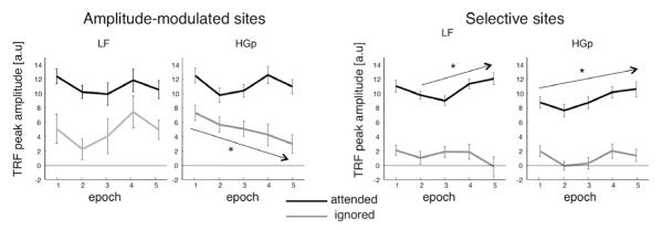
TRF peak amplitude (absolute value) for attended and ignored talkers across five successive epochs (3 seconds long, 1.5 second overlap). Results are shown separately for ‘amplitude-modulated’ and ‘selective’ sites, for both the LF and HGp TRFs. At selective sites, TRF responses for the attended increased significantly towards the end of the sentence, whereas at amplitude-modulated sites, the response remained consistent over the entire epoch. Arrows indicated significant monotonic changes over the course of the sentence.
Discussion
Using converging analytic approaches we confirm that both low-frequency phase (Ding and Simon, 2012b; Kerlin et al., 2010) and high-gamma power (Mesgarani and Chang, 2012) concurrently track the envelope of attended speech. Importantly, our data suggest that speech-tracking in these two bands reflects distinct neuronal mechanisms for auditory speech encoding, since they differed in their spatial distribution and response time course. Sites with significant tracking effects appear to fall into two categories: ‘Modulation’ sites show significant tracking of both talkers, albeit biased toward the attended one. ‘Selection’ sites show significant tracking of the attended talker, without detectable tracking of the ignored talker. Amplitude modulation is focused in and near STG, i.e. low-level auditory cortices, while selection has a wider topographic distribution that includes low-level auditory areas, as well as higher-order language processing and attentional control regions such as inferior frontal cortex, anterior and inferior temporal cortex and inferior parietal lobule. These findings provide new insight into the neural mechanisms for encoding continuous natural stimuli and how attention shapes the internal representation of these stimuli when they are task relevant.
‘Amplitude-Modulated’ vs. ‘Selective’ speech tracking
The spatial differences between ‘amplitude-modulated’ and ‘selective’ sites suggest that as input is transmitted from sensory regions to higher-order regions the representation becomes more selective. We recognize that rather than a dichotomy, these two types of attentional effects might reflect a continuum of attentional modulation, which becomes increasingly selective for the attended stimulus in higher-order regions. Nonetheless separating the recording sites according to these two types of attentional effects was a useful heuristic for characterizing their properties.
The distinction between ‘amplitude-modulated’ and ‘selective’ effects of attention contributes to the debates regarding the stage of attentional selection. The amplitude modulation effects observed in regions closer to auditory cortex are consistent with findings that sensory areas maintain representations for both attended and ignored speech (Ding and Simon, 2012b), as well as with classic findings for modulation of simple sensory responses by attention (Hillyard et al., 1973; Woldorff et al., 1993), which have been taken as evidence for ‘early selection’. However, the current results suggest that this selection is further refined at higher stages of processing, as additional information is accumulated, as indicated by the purely ‘selective’ responses found in higher order regions.
The more selective tracking of the attended talker is in line with the ‘Selective Entrainment Hypothesis’ (Schroeder and Lakatos, 2009b; Zion Golumbic et al., 2012), which posits that although at the level of auditory (sensory) cortex there are evoked responses to all detectable stimuli, selective entrainment of ambient low-frequency oscillations to the attended speech stream ensures that local neurons are in a high excitability state when key events in that stream arrive and thus these events are transmitted onward and generate neuronal responses, whereas most events in the ignored stream arrive at non-optimal excitability phases of the entrained oscillation, and are suppressed. Consistent with this view, low-frequency oscillations are often implicated in inter-areal communication (von Stein and Sarnthein, 2000) and specifically in gating the transfer of spiking activity within and between regions by constraining the temporal windows during which spikes can influence downstream activity (Buzsáki and Chrobak, 1995; Mazzoni et al., 2010; Schroeder and Lakatos, 2009a). Thus, low-frequency entrainment may serve as an ‘adaptive temporal filter’ which would severely attenuate or effectively eliminate sensory evoked responses to the ignored speech stream in downstream regions, while enhancing the representation and processing of the attended stream.
Another important distinction between ‘amplitude-modulated’ and ‘selective’ effects is how they change over the course of the sentence. Speech tracking of the attended talker in the ‘selective’ sites improved over the course of the sentence, indicating that these regions make use of accumulated spectro-temporal regularities (and perhaps prosodic/semantic cues as well) to dynamically refine their representation of the attended stimulus (Ahissar and Ahissar, 2005; Fritz et al., 2007; Ghitza, 2011; Xiang et al., 2010). In contrast, at ‘amplitude-modulated’ sites, the magnitude of the response to the attended stimulus remained constant throughout the epoch (Ding and Simon, 2012b).
Speech tracking using high-gamma power versus low-frequency phase
Our data show that both LF phase and HGp preferentially track the attended talker, and display both ‘amplitude-modulated’ and ‘selective’ effects. Moreover, we show that encoding in these frequency bands is not redundant. Indeed, there is increasing evidence that neural encoding of complex stimuli relies on the combination of local processing, manifest in single-unit and multi-unit activity, and slow fluctuations of synaptic current regulating the phase of populations excitability (Kayser et al., 2009; Mazzoni et al., 2010; Whittingstall and Logothetis, 2009). Not surprisingly, it is typically observed that neuronal firing amplitude, as indexed by MUA or HG power (Kayser et al., 2007; Nir et al., 2007) is coupled to the phase of lower frequency activity (Canolty and Knight, 2010; Lakatos et al., 2005b).
The relatively short latency of HGp speech tracking observed here (<50 ms), which reflects the lag between the stimulus and the neural response, is commensurate with latencies of evoked onset responses and MUA tracking latencies of sounds in auditory cortex (Elhilali et al., 2004; Lakatos et al., 2005a), supporting the association between HGp and local MUA. Conversely, LF speech tracking effects, particularly near auditory cortex, probably reflect a combination of low-frequency evoked responses (typically in the theta range; 4-7Hz, Howard and Poeppel, 2010; Mäkinen et al., 2005) and entrainment of low-frequency oscillations, discussed above. This distinction is important, since evoked responses typically show ‘amplitude-modulation’ attention effects (Woldorff et al., 1993), whereas entrainment is hypothesized as the basis for selective representation (Schroeder and Lakatos, 2009b). Concurrent multi-electrode recordings across the layers of monkey A1 and V1 demonstrate that selective LF entrainment and amplitude modulation of evoked response coexists and can be clearly distinguished, as they operate most strongly in different layers (Lakatos et al., 2008; Lakatos et al., 2009). Although it is methodologically difficult to separate these two processes on the ECoG-level, it is likely that the observed LF speech tracking effects near auditory cortex reflect a combination of these two responses, whereas ‘selective’ LF tracking reflects greater contribution of selective entrainment, commensurate with previous findings from our group (Besle et al., 2011). This claim is further supported by our supplementary data which show that LF tracking near auditory cortex contains a high contribution of theta-band activity, the dominant frequency in evoked responses, whereas the more widespread tracking in the high-order regions was dominated by lower frequencies (1-3Hz; as shown in Fig S3).
A previous ECoG study (Nourski et al., 2009) showed a distinction between HGp and LF speech tracking even within auditory cortex, suggesting that HGp reflects the bottom-up auditory response to the stimuli whereas LF tracking reflects processes more closely related to perception. In that study, HGp tracked the envelope of speech even when it was compressed beyond the point of intelligibility, whereas LF phase-locked to compressed speech only while it was still intelligible (see also Ahissar and Ahissar, 2005). These findings support the claim that LF speech tracking serves a role in gating and constraining the transfer of sensory responses (represented by HGp) to higher order regions according to attentional demands or processing capacity.
Contribution of Visual input
In our paradigm, participants viewed movies that contain both auditory and visual input. It is known that viewing a talking face contributes to speech processing, particularly under noisy auditory conditions (Bishop and Miller, 2008; Sumby and Pollack, 1954). Moreover, articulation movements of the mouth and jaw are correlated with the acoustic envelope of speech (Chandrasekaran et al., 2009; Grant and Seitz, 2000). Thus is it possible that, at least some of the speech-tracking effects reported here and driven or amplified by the visual input of the talking face. Indeed, we have recently shown that viewing a talking face enhances speech tracking in auditory cortex as well as selectivity for an attended speaker (Zion Golumbic et al., in press). The precise manner contribution of visual input to the speech-tracking response in different brain regions is an important question to be investigated in future research. Particularly, it would be important to determine whether the same set of brain regions track speech regardless of whether visual input is provided but the visual input enhances the magnitude of the tracking response, or whether visual input induces speech-tracking in additional brain areas.
Conclusions
Our results provide an empirical basis for the idea that selective attention in a ‘Cocktail Party’ setting relies on an interplay between bottom-up sensory responses and predictive, top-down control over the timing of neuronal excitability (Schroeder and Lakatos, 2009b). The product of this interaction is the formation of a dynamic neural representation of the temporal structure of the attended speech stream that functions as an amplifier and a temporal filter. This model can be applied to sensory responses in auditory cortex, to selectively amplify attended events and enhance their transmission to higher-level brain regions, while at the same time suppressing responses to ignored events. We furthermore show that as the sentence unfolds, the high-order representation for the attended talker is further refined. The combined attentional effects of top-down modulation of evoked responses and selective representation for the attended seen here are a compelling example of ‘Active Sensing’ (Schroeder et al., 2010; Zion Golumbic et al., 2012), a process in which the brain dynamically shapes its internal representation of stimuli, and particularly those of natural and continuous stimuli, according to environmental and contextual demands.
Experimental Procedures
Participants
Recordings were obtained from six patients with medically intractable epilepsy undergoing intracranial electrocorticographic (ECoG) recording to help identify the epileptogenic zone (4 patients at the Columbia University Medical Center/New York-Presbyterian Hospital - CUMC - and 2 patients at North Shore LIJ). These patients are chronically monitored with subdural electrodes for a period of one to four weeks, during which time they are able to participate in functional testing. The study was approved by the Institutional Review Boards of CUMC and North Shore/LIJ Health System. Informed consent was obtained from each patient prior to the experiment. All participants were right handed, with left-hemisphere dominance for language. They ranged in age between 21-45 (median age 26.5), and one participant was male. All participants were fluent in English.
Stimuli and Task
Stimuli consisted of movie clips of two talkers (one male, one female) reciting a short narrative (9-12 seconds long). The movies were edited using QuickTime Pro (Apple) to align the faces in the center of the frame, equate the relative size of the male and female faces, and to adjust the length of the movie. In addition the mean intensity of the audio was equated across all movies using Matlab (Mathworks, Natick, MA). Each female movie was paired with a male movie of similar length, and this pairing remained constant throughout the entire study (Supplementary Fig 2A). For 3 of the participants 6 movies were presented (3 male-female pairs) and for the other 3 participants 8 movies were presented (4 male-female pairs). The envelopes of all stimulus pairs were uncorrelated (Pearson correlation coefficient r <0.065 for all pairs).
The experiment was presented to the participants on a computer that was brought into their hospital room. Sounds were played through free field audio-speakers placed on either side of the computer screen, approximately 50cm from the subject. The volume was adjusted to a comfortable level, approximately 65dB SPL.
The experimental task consisted of a Cocktail Party block followed by a Single Talker block. In each Cocktail Party trial a female-male combination was presented with the two movies playing simultaneously on either side the computer screen. The location of each talker on the screen (left/right) was assigned randomly in each trial. However, the audio of both talkers was always played through both audio-speakers, so there was no spatial distinction between the two auditory streams. This was done in order to ensure that any attentional effects observed are entirely due to top-down selective attention and are not produced by a more general allocation of spatial attention.
Before each trial, instructions appeared in the center of the screen indicating which of the talkers to attend to (e.g. ‘Attend Female’). The participants indicated with a button press when they were ready to begin, and 2 seconds later the two videos started playing simultaneously. To assure the participants remembered which talker to attend to during the entire trial, the video of the attended talker was highlighted by a red frame (appearing with video onset). Each film was cut-off before the talker pronounced the last word, and then a target word appeared in the center of the screen. The participants’ explicit task was to indicate via button press whether the target word was a congruent ending to the attended narrative. An example narrative and target words: “My best friend, Jonathan, has a pet parrot who can speak. He can say his own name and call out ‘Hello, come on it’ whenever he hears someone ringing the… ”, Target words: doorbell (congruent); table (incongruent). Target words were unique on each trial (no repetitions), and 50% were congruent with the attended segment.
The Single Talker trials were identical to the Cocktail Party trials, however instead of presenting both talkers simultaneously, only the attended talker was audible while the sound track of the other talker was muted. The task remained the same in the Single Talker block. Each individual film was presented 8-10 times each block and was designated as the “attended” film in half of the repetitions. The order of the stimuli and target words was randomized within each block, and breaks were given every 10 trials.
Data acquisition
Participants were implanted with clinical subdural electrodes, which are platinum disks 4-5mm (2.5mm exposed) in diameter and arranged in linear or matrix arrays with 1 cm center to center spacing. All participants had between 112-128 electrodes implanted, including an array of 32-64 electrodes over temporo-parietal or temporo-frontal regions as well as several strips of 4-8 electrodes in various additional locations. 4 Participants had a left-sided implant and the locations of electrodes from individual participants are shown in Supplementary Fig 1. Intracranial EEG was acquired at 1000 or 2000 Hz/channel sampling rate with 24-bit precision (0.5 – 500/1000 Hz bandpass filtering) using a clinical video-EEG system (XLTek Inc., Oakville, Ontario, Canada). All ECoG recordings were then resampled to 1 kHz offline. For CUMC patients, the reference was an inverted electrode strip positioned over the electrode grid, with electrical contacts facing the dura. For LIJ patients, both the reference and ground electrodes were attached to the skull, on the frontal bone approximately at midline.
Electrode localization
The location of the electrodes relative to the cortical surface was determined using Bioimagesuite software (http://www.bioimagesuite.org) and custom-made Matlab (Mathworks, Natick, MA) scripts. Post-implantation CT scans were thresholded to identify the electrode locations in the coordinate system of the CT scan. As a first approach to localization relative to the cortex, we co-registered the CT scan volume to the pre-operative MR volume by linear transformation using an automated procedure and transformed the coordinates of the electrodes into the coordinate system of the pre-operative MR. Because of the tissue compression and the small degree of midline shift (usually less than 2 cm) that typically occurs during subdural array implantation, the result of this co-registration is approximate. To minimize this shift, when a post-operative MR volume was available (3 out of 6 participants), the CT scan was first co-registered to the post-operative MR and then to the pre-operative MR using a linear transformation matrix between the pre- and post-operative MRs.
Since we focus on group analysis in this paper, we co-registered the best available MR to the MNI 152 standard brain (http://imaging.mrc-cbu.cam.ac.uk/imaging/MniTalairach), and all electrodes are displayed on a 3D reconstruction of the cortical surface of the MNI brain. Finally, for display purposes, in the main Figs right-sided electrodes (from two patients) are displayed on homotopic brain areas on the left hemisphere.
ECoG Signal processing
All analyses were performed using Matlab. Electrodes with persistent abnormal activity or frequent interictal epileptiform discharges were excluded from the analysis, yielding a total of 479 channels that were included in the analysis (67-89 good channels per participant; see Supplementary Fig 1). Due to the long duration of stimuli (> 9 sec), we did not reject trials that contained non-physiological artifacts or infrequent interictal epileptiform discharges (this policy only lowers predictability results, and is therefore conservative). The raw data was segmented into trials starting 4 sec prior to stimulus onset and lasting for 16 sec post-stimulus, so as to include the entire duration of all stimuli and to avoid contamination of edge effects due to subsequent filtering.
Inter-trial Coherence (ITC)
To determine whether a neural response is consistent across repetitions of the same stimulus, we calculated the phase coherence spectrum and the inter-trial coherence (ITC). For the phase coherence spectrum, we applied the Fourier transform to the neural responses (1 Hz resolution) and extracted the response phase at each frequency. The coherence of the response phase over repetitions of the same stimulus is then calculated using circular statistics. To estimate the chance level, we also calculated the phase coherence over responses to different stimuli.
For the phase-ITC and power-ITC, we filtered the neural response is into six frequency bands (delta 1-3 Hz, theta 4-7 Hz, alpha 8-12 Hz, beta 12-20 Hz, gamma 30-50 Hz, high-gamma 70-150 Hz). We then calculated the correlation coefficient across the responses in different trials, separately for the filtered waveforms (to obtain phase-ITC) and power waveforms (root-mean square of the filtered waveform; to obtain power-ITC). In the Single Talker condition, two types of ITC were calculated: 1) the Same-Stimulus ITC (the correlation between every pair of responses to the same stimulus), and 2) the Different-Stimuli ITC (the correlation between every pair of responses to different stimuli). Significant stimulus-locked responses are determined by comparing the within-stimulus correlation and the across-stimuli correlation using an unpaired t-test. In the Cocktail Party condition, three types of ITC were calculated: 1) the Same-Pair, Attend-Same ITC (the correlation between responses to the same stimulus under the same attentional focus), 2) the Same-Pair, Attend-Different ITC (the correlation between responses to the same stimulus under different attentional foci), and 3) the Different-Stimuli ITC. Significant attentional modulations are determined by comparing the Same-Pair, Attend-Same correlation and the Same-Pair, Attend-Different correlation using a paired t-test.
Speech Envelope Reconstruction
The temporal envelope of each stream of speech was reconstructed by linearly integrating the neural response over electrodes and time:
where rk(t) and ŝ(t) are the ECoG signal in electrode k and the reconstructed envelope, and h(t) is a weighting matrix called the decoder. The time lag τ is limited to the range between 0 and 500 ms. Since reliable neural response were only observed below 10 Hz (Fig 1A), the response and stimulus were downsampled to 50 Hz. Only electrodes showing a significant inter-trial correlation (p < 0.001 uncorrected, either in the Single Talker condition or in the Cocktail Party condition, for ECoG activity below 10 Hz) were included. The ECoG signal rk(t) is either the low-frequency response waveform or the high-gamma power.
The decoder, h(t), was estimated using boosting with 10-fold cross validation (David et al., 2007) to minimize the mean square error between the reconstructed envelope and the actual envelope of a talker. The reconstructions start with a null vector as the initial condition for boosting. All the stimuli and responses were concatenated over stimuli in the analysis. The reconstruction accuracy was evaluated as the correlation coefficient between the reconstructed envelope and the actual envelope of the speech stream. To evaluate the significance level of the reconstruction, the concatenated stimulus was cut into 10 equal-length segments and the 10 segments are shuffled. A pseudo-reconstruction was then done based on the shuffled stimulus and the actual response (not shuffled). This shuffling and pseudo-reconstruction were done 1000 times to estimate the null distribution of the reconstruction accuracy.
Temporal Response Function
To determine the relationship between the neural response and the presented speech stimuli we estimated a linear Temporal Response Function (TRF) between the stimulus and the response. The neural response r(t) is modeled by the temporal envelope of the presented talker s(t):
The TRF(t) is a linear kernel and ε(t) is the residual response not explained by the model (Theunissen et al., 2001). The broadband envelope of speech s(t) was extracted by filtering the speech stimuli in 64-frequency bands spaced logarithmically between 500-2000 Hz, extracting the temporal envelope in each band using a Hilbert transform and then averaging across the narrow-band envelopes.
The temporal response functions TRF(t) were fitted using normalized reverse correlation as implemented in the STRFpak Matlab toolbox (http://strfpak.berkeley.edu/). Normalized reverse correlation involves inverting the autocorrelation matrix of the stimulus, which is usually numerically ill-conditioned. Therefore, a pseudo-inverse is applied instead, which ignores eigenvalues of the autocorrelation matrix that are smaller than a pre-defined tolerance factor. The tolerance factor was scanned and determined by a pre-analysis to optimize the predictive power and then fixed for all electrodes.
We chose to use the broadband speech envelope to model the neural response, rather than a series of narrow band envelopes since our coarse spatial resolution of ECoG (~1cm) would make distinguishing between neuronal populations tracking narrow-band envelopes unlikely. We estimated the TRF separately for each electrode, using either the low-frequency ECoG response or the HGp time course. Single trial responses were averaged over trials (with the same stimuli) and concatenated over stimuli prior to model estimation. In the Cocktail Party condition, we modeled the neural response r(t) by the temporal envelopes of both the attended and ignored talkers (sA(t) and sI(t) respectively), generating a temporal response function for each talker (TRFA and TRFI , respectively).
| (3) |
If the two films presented in the same trial had different lengths, only the portion of the stimulus that overlapped in time was included in the model, and the response r(t) to that stimulus pair was truncated accordingly.
The TRFs were 300 ms long and were estimated using a jackknife cross-validation procedure, to minimize effects of over-fitting (Ding and Simon, 2012b). In this procedure, given a total of N stimuli, a TRF is estimated between s(t) and r(t) derived from N-1 stimuli, and this estimate is used to predict the neural response to the left-out stimulus. Since each stimulus is between 9-12 seconds long, and each subject had 6 or 8 different stimuli, each jackknife estimation of the TRF was made using 50 – 80 seconds of data. The goodness of fit of the model was evaluated by the correlation between the actual neural response and the model prediction, called predictive power (David et al., 2007). The predictive power calculated from each jackknife estimate is averaged.
To evaluate whether the predictive power of a particular TRF estimate is statistically significant, we repeated the cross-validation procedure 1000 times for each electrode, substituting the observed response in the left-out trial with a random portion of the data from that electrode to create a null-distribution of predictive power values. Electrodes whose predictive power fell in the top 1%tile of the null distribution were considered significant (electrode-wise significance p<0.01). Since performing multiple statistical tests can increase the probability of false-positives, we evaluated the group-wise significance value that reflects the chance to get X significant electrodes, given N tests. This was done by a) counting the number of significant electrodes (p<0.01) in each of the 1000 data-permutations, and b) creating a second null-distribution of the number of significant electrodes you might get by chance. The number of significant electrodes in the original data set was compared to this group-wise distribution and group-wise p-values were calculated as the proportion of null-values exceeding the value observed in the original data set. Permutation tests and group-wise p-values were calculated separately for each participant, thus the numerical threshold for significant predictive-power values could differ across participants. This was done since not all participants had the same number of stimuli/trials and thus differed in their signal-to-noise, so applying the same threshold to all participants might be too conservative.
In the Cocktail Party condition we calculated the predictive power separately for the attended and ignored stimuli by calculating the correlation between actual neural response and the prediction made the TRF estimated from stimulus, i.e. and . The permutation tests yielded separate null-distributions for attended and ignored, however in order to avoid using two different statistical thresholds, we chose the higher of the two thresholds (p<0.01) to evaluate the significance of both the attended and ignored TRFs at each site. Evaluation of the group-wise statistic was done in the same way. Using the same data-driven statistical threshold for both attended and ignored enabled us to distinguish between electrodes where the predictive power was significant for both attended and ignored stimuli (‘Amplitude-Modulated’ electrodes) vs electrodes where only the predictive power of the attended passed the statistical threshold (‘Selective’ electrodes; Fig 6).
To evaluate the similarity between TRF morphology for attended and ignored stimuli, we calculated the Pearson correlation at each site and averaged across ‘Selective’ and ‘Amplitude-Modulated’ sites separately. For each electrode and condition we assessed the peak of the TRF as the peak with the highest absolute value. Since the polarity of the TRF peaks is inconsequential (influenced by the location of the recording site relative to the neural generator), we corrected the sign of the peak TRF amplitude in the Cocktail Party condition according to the attended talker, which allowed us to pool the value across sites and to compare response to attended and ignored stimuli and asses attentional effects (Figs 4,6&7).
To evaluate how the TRF changes over the duration of a trial (Fig 7), we estimated the TRF as above but using shorter epochs. We used 3-second long epochs with a 1.5 second overlap yielding a total of 5 epochs between 0 – 9 seconds (since the shortest stimulus was 9 seconds long). In each epoch we identified the peak of the TRF for the attended and ignored (sign corrected as described above). To test whether the response to attended and ignored stimuli changed over the course of the 5 epochs, we first normalized the TRF amplitude values at each site by subtracting the mean TRF amplitude across all epochs. We then used a Mann-Kendall Tau test to determine whether there was a significant monotonic trend of the TRF amplitudes over the course of the sentence. This analysis was performed separately for ‘Selective’ and ‘Amplitude-Modulated’ sites, in each band.
Supplementary Material
Highlights.
Both low-frequency phase and high-gamma power preferentially track attended speech
Near auditory cortex attention modulates response to attended and ignored talkers
Selective tracking of only the attended talker increases in higher order regions
Selective tracking of the attended talker increases over time
Acknowledgments
This work was supported by MH093061, MH60358, MH086385, DC008342, and DC05660. We thank Dr. Joseph Isler and the other members of the Columbia Oscillations Journal Club for critical comments and advice on this work.
Footnotes
Publisher's Disclaimer: This is a PDF file of an unedited manuscript that has been accepted for publication. As a service to our customers we are providing this early version of the manuscript. The manuscript will undergo copyediting, typesetting, and review of the resulting proof before it is published in its final citable form. Please note that during the production process errors may be discovered which could affect the content, and all legal disclaimers that apply to the journal pertain.
References
- Ahissar E, Ahissar M. Processing of the Temporal Envelope of Speech. In: Konig R, Heil P, Budinger E, Scheich H, editors. The Auditory Cortex: A Synthesis of Human and Animal Research. Lawrence Erlbaum Associates, Inc; London: 2005. pp. 295–313. [Google Scholar]
- Ahveninen J, Hämäläinen M, Jääskeläinen IP, Ahlfors SP, Huang S, Lin F-H, Raij T, Sams M, Vasios CE, Belliveau JW. Attention-driven auditory cortex short-term plasticity helps segregate relevant sounds from noise. Proceedings of the National Academy of Sciences. 2011;108:4182–4187. doi: 10.1073/pnas.1016134108. [DOI] [PMC free article] [PubMed] [Google Scholar]
- Belitski A, Panzeri S, Magri C, Logothetis NK, Kayser C. Sensory information in local field potentials and spikes from visual and auditory cortices: time scales and frequency bands. J Comput Neurosci. 2010;29:533–545. doi: 10.1007/s10827-010-0230-y. [DOI] [PMC free article] [PubMed] [Google Scholar]
- Besle J, Schevon CA, Mehta AD, Lakatos P, Goodman RR, McKhann GM, Emerson RG, Schroeder CE. Tuning of the Human Neocortex to the Temporal Dynamics of Attended Events. J Neurosci. 2011;31:3176–3185. doi: 10.1523/JNEUROSCI.4518-10.2011. [DOI] [PMC free article] [PubMed] [Google Scholar]
- Bishop CW, Miller LM. A Multisensory Cortical Network for Understanding Speech in Noise. J Cognit Neurosci. 2008;21:1790–1804. doi: 10.1162/jocn.2009.21118. [DOI] [PMC free article] [PubMed] [Google Scholar]
- Buzsaki G. Rhythms of the Brain. Oxford University Press; Oxford, New York: 2006. [Google Scholar]
- Buzsáki G, Chrobak JJ. Temporal structure in spatially organized neuronal ensembles: a role for interneuronal networks. Curr Opin Neurobiol. 1995;5:504–510. doi: 10.1016/0959-4388(95)80012-3. [DOI] [PubMed] [Google Scholar]
- Canolty RT, Knight RT. The functional role of cross-frequency coupling. Trends Cogn Sci. 2010;14:506–515. doi: 10.1016/j.tics.2010.09.001. [DOI] [PMC free article] [PubMed] [Google Scholar]
- Chandrasekaran C, Trubanova A, Stillittano S.b., Caplier A, Ghazanfar AA. The Natural Statistics of Audiovisual Speech. PLoS Comput Biol. 2009;5:e1000436. doi: 10.1371/journal.pcbi.1000436. [DOI] [PMC free article] [PubMed] [Google Scholar]
- Cherry EC. Some experiments on the recognition of speech, with one and two ears. J Acoust Soc Am. 1953;25:975–979. [Google Scholar]
- David SV, Mesgarani N, Shamma SA. Estimating sparse spectro-temporal receptive fields with natural stimuli. Network: Comput Neural Syst. 2007;18:191–212. doi: 10.1080/09548980701609235. [DOI] [PubMed] [Google Scholar]
- Ding N, Simon JZ. Emergence of neural encoding of auditory objects while listening to competing speakers. Proceedings of the National Academy of Sciences. 2012a;109:11854–11859. doi: 10.1073/pnas.1205381109. [DOI] [PMC free article] [PubMed] [Google Scholar]
- Ding N, Simon JZ. Neural Coding of Continuous Speech in Auditory Cortex during Monaural and Dichotic Listening. J Neurophysiol. 2012b;107:78–89. doi: 10.1152/jn.00297.2011. [DOI] [PMC free article] [PubMed] [Google Scholar]
- Elhilali M, Fritz JB, Klein DJ, Simon JZ, Shamma SA. Dynamics of Precise Spike Timing in Primary Auditory Cortex. J Neurosci. 2004;24:1159–1172. doi: 10.1523/JNEUROSCI.3825-03.2004. [DOI] [PMC free article] [PubMed] [Google Scholar]
- Elhilali M, Xiang J, Shamma SA, Simon JZ. Interaction between Attention and Bottom-Up Saliency Mediates the Representation of Foreground and Background in an Auditory Scene. PLoS Biol. 2009;7:e1000129. doi: 10.1371/journal.pbio.1000129. [DOI] [PMC free article] [PubMed] [Google Scholar]
- Fritz JB, Elhilali M, David SV, Shamma SA. Auditory attention -- focusing the searchlight on sound. Curr Opin Neurobiol. 2007;17:437–455. doi: 10.1016/j.conb.2007.07.011. [DOI] [PubMed] [Google Scholar]
- Ghitza O. Linking speech perception and neurophysiology: speech decoding guided by cascaded oscillators locked to the input rhythm. Frontiers in Psychology: Auditory Cognitive Neuroscience. 2011;2:130. doi: 10.3389/fpsyg.2011.00130. doi: 10.3389/fpsyg.2011.00130. [DOI] [PMC free article] [PubMed] [Google Scholar]
- Giraud A-L, Poeppel D. Cortical oscillations and speech processing: emerging computational principles and operations. Nat Neurosci. 2012;15:511–517. doi: 10.1038/nn.3063. [DOI] [PMC free article] [PubMed] [Google Scholar]
- Grant KW, Seitz P-F. The use of visible speech cues for improving auditory detection of spoken sentences. J Acoust Soc Am. 2000;108:1197–1208. doi: 10.1121/1.1288668. [DOI] [PubMed] [Google Scholar]
- Greenberg S, Ainsworth W. Listening to Speech: an Auditory Perspective. Erlbaum; Mahwah, NJ: 2006. [Google Scholar]
- Hillyard S, Hink R, Schwent V, Picton T. Electrical signs of selective attention in the human brain. Science. 1973;182:177–180. doi: 10.1126/science.182.4108.177. [DOI] [PubMed] [Google Scholar]
- Howard MF, Poeppel D. Discrimination of Speech Stimuli Based on Neuronal Response Phase Patterns Depends on Acoustics But Not Comprehension. J Neurophysiol. 2010;104:2500–2511. doi: 10.1152/jn.00251.2010. [DOI] [PMC free article] [PubMed] [Google Scholar]
- Kayser C, Montemurro MA, Logothetis NK, Panzeri S. Spike-Phase Coding Boosts and Stabilizes Information Carried by Spatial and Temporal Spike Patterns. Neuron. 2009;61:597–608. doi: 10.1016/j.neuron.2009.01.008. [DOI] [PubMed] [Google Scholar]
- Kayser C, Petkov C, Logothetis NK. Tuning to sound frequency in auditory field potentials. J Neurophysiol. 2007;98:1806–1809. doi: 10.1152/jn.00358.2007. [DOI] [PubMed] [Google Scholar]
- Kerlin JR, Shahin AJ, Miller LM. Attentional Gain Control of Ongoing Cortical Speech Representations in a “Cocktail Party”. J Neurosci. 2010;30:620–628. doi: 10.1523/JNEUROSCI.3631-09.2010. [DOI] [PMC free article] [PubMed] [Google Scholar]
- Lakatos P, Karmos G, Mehta AD, Ulbert I, Schroeder CE. Entrainment of Neuronal Oscillations as a Mechanism of Attentional Selection. Science. 2008;320:110–113. doi: 10.1126/science.1154735. [DOI] [PubMed] [Google Scholar]
- Lakatos P, O’Connell MN, Barczak A, Mills A, Javitt DC, Schroeder CE. The Leading Sense: Supramodal Control of Neurophysiological Context by Attention. Neuron. 2009;64:419–430. doi: 10.1016/j.neuron.2009.10.014. [DOI] [PMC free article] [PubMed] [Google Scholar]
- Lakatos P, Pincze Z, Fu K, Javitt DC, Karmos G, Schroeder CE. Timing of pure tone and noise-evoked responses in macaque auditory cortex. Neuroreport. 2005a;16:933–937. doi: 10.1097/00001756-200506210-00011. [DOI] [PubMed] [Google Scholar]
- Lakatos P, Shah AS, Knuth KH, Ulbert I, Karmos G, Schroeder CE. An Oscillatory Hierarchy Controlling Neuronal Excitability and Stimulus Processing in the Auditory Cortex. J Neurophysiol. 2005b;94:1904–1911. doi: 10.1152/jn.00263.2005. [DOI] [PubMed] [Google Scholar]
- Large EW, Jones MR. The dynamics of attending: How people track time-varying events. Psychol Rev. 1999;106:119–159. [Google Scholar]
- Luo H, Poeppel D. Phase Patterns of Neuronal Responses Reliably Discriminate Speech in Human Auditory Cortex. Neuron. 2007;54:1001–1010. doi: 10.1016/j.neuron.2007.06.004. [DOI] [PMC free article] [PubMed] [Google Scholar]
- Mäkinen V, Tiitinen H, May P. Auditory event-related responses are generated independently of ongoing brain activity. NeuroImage. 2005;24:961–968. doi: 10.1016/j.neuroimage.2004.10.020. [DOI] [PubMed] [Google Scholar]
- Mazzoni A, Whittingstall K, Brunel N, Logothetis NK, Panzeri S. Understanding the relationships between spike rate and delta/gamma frequency bands of LFPs and EEGs using a local cortical network model. NeuroImage. 2010;52:956–972. doi: 10.1016/j.neuroimage.2009.12.040. [DOI] [PubMed] [Google Scholar]
- Mesgarani N, Chang EF. Selective cortical representation of attended speaker in multi-talker speech perception. Nature. 2012;485:233–236. doi: 10.1038/nature11020. [DOI] [PMC free article] [PubMed] [Google Scholar]
- Nir Y, Fisch L, Mukamel R, Gelbard-Sagiv H, Arieli A, Fried I, Malach R. Coupling between Neuronal Firing Rate, Gamma LFP, and BOLD fMRI Is Related to Interneuronal Correlations. Curr Biol. 2007;17:1275–1285. doi: 10.1016/j.cub.2007.06.066. [DOI] [PubMed] [Google Scholar]
- Nourski KV, Reale RA, Oya H, Kawasaki H, Kovach CK, Chen H, Howard MA, Brugge JF. Temporal Envelope of Time-Compressed Speech Represented in the Human Auditory Cortex. J Neurosci. 2009;29:15564–15574. doi: 10.1523/JNEUROSCI.3065-09.2009. [DOI] [PMC free article] [PubMed] [Google Scholar]
- Pasley BN, David SV, Mesgarani N, Flinker A, Shamma SA, Crone NE, Knight RT, Chang EF. Reconstructing Speech from Human Auditory Cortex. PLoS Biol. 2012;10:e1001251. doi: 10.1371/journal.pbio.1001251. [DOI] [PMC free article] [PubMed] [Google Scholar]
- Rosen S. Temporal Information in Speech: Acoustic, Auditory and Linguistic Aspects. Phil Trans Biol Sci. 1992;336:367–373. doi: 10.1098/rstb.1992.0070. [DOI] [PubMed] [Google Scholar]
- Schroeder CE, Lakatos P. The Gamma Oscillation: Master or Slave? Brain Topogr. 2009a;22:24–26. doi: 10.1007/s10548-009-0080-y. [DOI] [PMC free article] [PubMed] [Google Scholar]
- Schroeder CE, Lakatos P. Low-frequency neuronal oscillations as instruments of sensory selection. Trends Neurosci. 2009b;32:9–18. doi: 10.1016/j.tins.2008.09.012. [DOI] [PMC free article] [PubMed] [Google Scholar]
- Schroeder CE, Wilson DA, Radman T, Scharfman H, Lakatos P. Dynamics of Active Sensing and perceptual selection. Curr Opin Neurobiol. 2010;20:172–176. doi: 10.1016/j.conb.2010.02.010. [DOI] [PMC free article] [PubMed] [Google Scholar]
- Shannon RV, Zeng F-G, Kamath V, Wygonski J, Ekelid M. Speech Recognition with Primarily Temporal Cues. Science. 1995;270:303–304. doi: 10.1126/science.270.5234.303. [DOI] [PubMed] [Google Scholar]
- Stefanics G, Hangya B, Hernádi I, Winkler I, Lakatos P, Ulbert I. Phase Entrainment of Human Delta Oscillations Can Mediate the Effects of Expectation on Reaction Speed. J Neurosci. 2010;30:13578–13585. doi: 10.1523/JNEUROSCI.0703-10.2010. [DOI] [PMC free article] [PubMed] [Google Scholar]
- Sumby WH, Pollack I. Visual contribution to speech intelligibility in noise. J Acoust Soc Am. 1954;26:212–215. [Google Scholar]
- Theunissen FE, David SV, Singh NC, Hsu A, Vinje WE, Gallant JL. Estimating spatio-temporal receptive fields of auditory and visual neurons from their responses to natural stimuli. Network: Comput Neural Syst. 2001;12:289–316. [PubMed] [Google Scholar]
- von Stein A, Sarnthein J. Different frequencies for different scales of cortical integration: from local gamma to long range alpha/theta synchronization. Int J Psychophysiol. 2000;38:301–313. doi: 10.1016/s0167-8760(00)00172-0. [DOI] [PubMed] [Google Scholar]
- Whittingstall K, Logothetis NK. Frequency-Band Coupling in Surface EEG Reflects Spiking Activity in Monkey Visual Cortex. Neuron. 2009;64:281–289. doi: 10.1016/j.neuron.2009.08.016. [DOI] [PubMed] [Google Scholar]
- Woldorff MG, Gallen CC, Hampson SA, Hillyard SA, Pantev C, Sobel D, Bloom FE. Modulation of early sensory processing in human auditory cortex during auditory selective attention. Proceedings of the National Academy of Sciences. 1993;90:8722–8726. doi: 10.1073/pnas.90.18.8722. [DOI] [PMC free article] [PubMed] [Google Scholar]
- Wood N, Cowan N. The cocktail party phenomenon revisited: How frequent are attention shifts to one’s name in an irrelevant auditory channel? Journal of Experimental Psychology: Learning, Memory, and Cognition. 1995;21:255–260. doi: 10.1037//0278-7393.21.1.255. [DOI] [PubMed] [Google Scholar]
- Xiang J, Simon J, Elhilali M. Competing Streams at the Cocktail Party: Exploring the Mechanisms of Attention and Temporal Integration. J Neurosci. 2010;30:12084–12093. doi: 10.1523/JNEUROSCI.0827-10.2010. [DOI] [PMC free article] [PubMed] [Google Scholar]
- Zion Golumbic EM, Cogan GB, Schroeder CE, Poeppel D. Visual Input Enhances Selective Speech Envelope Tracking in Auditory Cortex at a ‘Cocktail Party’. J Neurosci. doi: 10.1523/JNEUROSCI.3675-12.2013. (in press) [DOI] [PMC free article] [PubMed] [Google Scholar]
- Zion Golumbic EM, Poeppel D, Schroeder CE. Temporal Context in Speech Processing and Attentional Stream Selection: A Behavioral and Neural perspective. Brain Lang. 2012;122:151–161. doi: 10.1016/j.bandl.2011.12.010. [DOI] [PMC free article] [PubMed] [Google Scholar]
Associated Data
This section collects any data citations, data availability statements, or supplementary materials included in this article.