Practical recommendations for population PK studies with sampling time errors

Abstract

Purpose

Population pharmacokinetic (PK) data collected from routine clinical practice offers a rich source of valuable information. However, in observational population PK data, accurate time information for blood samples is often missing, resulting in measurement errors (ME) in the sampling time variable. The goal of this study was to investigate the effects on model parameters when a scheduled time is used instead of the actual blood sampling time, and to propose ME correction methods.

Methods

Simulation studies were conducted based on two major factors: the curvature in PK profiles and the size of ME. As ME correction methods, transform both sides (TBS) models were developed with application of Box-Cox power transformation and Taylor expansion. The TBS models were compared to a conventional population PK model using simulations.

Results

The most important determinant of bias due to time ME was the degree of curvature (nonlinearity) in PK profiles; the smaller the curvature around sampling times, the smaller the associated bias. The second important determinant was the magnitude of ME; the larger the ME, the larger the bias. The proposed TBS models performed better than a conventional population PK modeling when curvature and ME were substantial.

Conclusions

Time ME in sampling time can lead to bias on the parameter estimators. The following practical recommendations are provided: 1) when the curvature of PK profiles is small, conventional population PK modeling is robust to even large ME; and 2) when the curvature is moderate or large, the proposed methodology reduces bias in parameter estimates.

Introduction

Observational population pharmacokinetic (PK) data collected during routine clinical practice is a potentially rich source of valuable information. In contrast to PK data collected from a clinical trial or a well-controlled environment, the analysis of observational population PK data poses several statistical challenges. Our focus lies on the issue of measurement error (ME) in blood sampling times in population PK modeling, which can occur for multiple reasons. For example, blood sampling times could be set to a scheduled or lab test time, which may be quite different from the actual blood draw time. Moreover, blood draw times may be completely missing or inaccurately recorded due to other factors. Since pharmacokinetics studies the time course of drugs, time information about blood sample draws or drug administration is a critical data component. As blood draw time is not accurately recorded in many observational PK studies, there is thus a need for methods that take such errors into account and provide general recommendations to practitioners.

Examples where this problem is apparent include population PK or pharmacogenetic studies for immunosuppressive drugs such as cyclosporin or tacrolimus [1, 2] and for the anticoagulant drug warfarin [3] with data collected via therapeutic drug monitoring. These drugs have a narrow therapeutic index and high inter-individual variation in their PK profiles. Thus, drug concentration is routinely monitored to ensure that it is maintained within the proper therapeutic range. Several tacrolimus PK studies have been performed using trough concentrations that were intended to be assessed at a specified time before the morning dose. Without recording the exact time of the blood draw, the time for concentration in the PK modeling is assumed to be either 1 hour or just before the dose. Hence, the time variable used in PK modeling is actually different from the true sampling time. Although detailed information about how the sampling time collection is frequently missing, many population PK or pharmacogenetic studies, especially those performed using data collected from routine clinical care with sparse sampling, are likely to use a scheduled time as erroneously reported in the data set; that is, the sampling time, which is a predictor variable, is measured with error from a statistical modeling perspective.

There are two major common cases of ME associated with predictor variables in a statistical model, classical and Berkson [4], their differences well- described in Carroll et al. [5]. The ME present in a scheduled time variable in PK modeling belongs to the Berkson error type, in the sense that the variability in the true sampling time is larger than that of the scheduled time [5]. Measurement error in predictor variables in regression analysis has been studied over several decades. The effect of ME in covariates in linear, nonlinear, and mixed effects regression models is now well understood [5–12]. The literature on ME in nonlinear mixed effects models is also developed [13–15].

However, very little work has been done for the case when ME is present in the sampling time in population PK models. A notable exception is Wang and Davidian [16], who calculated the theoretical bias due to ME in the scheduled time. Their simulation studies indicated that the bias is very small for the major PK parameters, partially contradicting their theoretical findings, which predicted a much higher substantial bias. This might be due to the dense sampling design (i.e., 8 time points over 24 h at scheduled times) used in their simulations, as such a design is atypical for population PK data. Thus, this manuscript closes the gap between the theoretical and simulation results via more realistic population PK sampling designs.

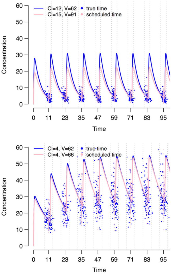
In order to provide additional insight into how ME in scheduled time could affect the estimated PK profiles (i.e., PK parameters), consider the example in Fig. 1. For illustrative purposes, two scenarios were selected based on the magnitude of clearance (CL) with volume of distribution (V) being held fixed at 60 l and the size of ME, specified in terms of its standard deviation, σ_u. Representative simulated data sets of 100 subjects with the true sampling times (blue dots) and the same data with the true sampling times being replaced by the scheduled times (pink dots) were fit, and the estimated population mean PK profiles in the same color are presented along with their estimated values in the upper panel (fast clearance CL =12.6 l h⁻¹; moderate ME σ_u =1 h) and the bottom panel (slow clearance CL =4.2 l h⁻¹; large ME σ_u =1.5 h). The simulation design will be described in detail in the methods section, which mimics a tacrolimus population PK study. The example illustrates that when the clearance is large, bias in PK parameter estimates can be very large, even with a moderate ME of σ_u being equal to 1 h. This is “moderate” in the sense that most true sampling times are within 2 hours of the scheduled times, represented by the dotted gray lines. Accordingly, the estimated PK profile can substantially deviate from the true profile. On the other hand, in the slow clearance case, the bias is far less obvious in spite of the sizeable ME (σ_u =1.5 h).

Fig. 1.

Population mean profiles estimated using the true sampling times and the scheduled times from representative simulated data sets with 100 subjects. For the simulation, two scenarios of true PK parameters were used for illustrative purpose: CL=12.6 l h⁻¹ for fast clearance and CL=4.2 l h⁻¹ for slow clearance (both with V =60 l being held fixed). Also moderate (with fast clearance) or large (with slow clearance) time ME was assumed. The simulated data sets with the true sampling times (blue dots) and the same data with the true sampling times being replaced by the scheduled times (pink dots) were fit, and the estimated population mean PK profiles in the same color are presented along with their estimated numerical values shown within the figure. Upper panel: fast clearance CL=12.6 l h⁻¹ with moderate time ME σ_u =1 h; bottom panel: slow clearance CL =4.2 l h⁻¹ with large time ME σ_u =1.5 h, where σ_u is the standard deviation of time ME. The dotted gray lines represent the scheduled sampling times ±2σ_u, where most true sampling times would lie within these lines

It is commonly recognized that Berkson error does not affect the bias of the point estimators in linear regression, though it does inflate the standard error of the slope estimator. This fact is often misinterpreted as a license to ignore Berkson error in a regression analysis. However, the exact effect of Berkson error in nonlinear models remains largely unknown. Here we focus on PK models—which are inherently highly nonlinear—demonstrating that Berkson error can lead to biased estimators in PK settings, and we propose a method for improvement. Recommendations are provided, along with a guideline for instances when a conventional PK modeling could be performed using the scheduled blood sampling time as if it is true, and when a ME correction method should be used to reduce bias due to time ME. The goal is to provide simple, clear recommendations for population PK study design and analysis.

Methods

A conventional population PK model

We set up the notation for a general population PK model and describe the true model used in simulation studies. Suppose that drug plasma concentration, y_ij, is measured on individual i, i =1, …, N, at the j^th time x_ij, j =1, …, m_i.

At the first stage, we describe drug concentration-time profile for individual i, predicted by a nonlinear function f (θ_i, x_ij) with the i^th individual parameters θ_i. A common assumption for the residual errors can be given below, which is used in our simulation studies:

$$y_{ij}=f({\mathit{\theta }}_{\mathit{i}},x_{ij})+\sigma f({\mathit{\theta }}_{\mathit{i}},x_{ij}){\epsilon }_{ij},$$ (1)

where ε_ij are independently and normally distributed with zero mean and unit variance, ε_ij ~N(0, 1).

At the second stage, distributions for the individual PK parameters are defined, with the most commonly used distributional assumption being a multivariate lognormal distribution. Let θ_i =(θ_1i, θ_2i, …, θ_pi) denote a p–vector of logarithmic transformed parameters specific to the individual i, and Z_i be a design matrix that may include the i^th individual’s covariates. Then, θ_i =Z_iθ+b_i, b_i ~MVN(0, Ω), where θ are a p–vector of fixed parameters and b_i is a p–vector of random effects, and the MVN stands for a multivariate normal with mean vector 0 and covariance matrix Ω. For the simulation studies, Z_i includes only the intercept, while a one-compartmental PK model with first order absorption is assumed with the absorption rate constant k_a being held fixed at 4.5 h⁻¹ as commonly done in the tacrolimus population PK studies. Hence, fixed effects are e^θ=(CL, V), where CL is clearance and V is volume of distribution, and the random effects variance components are

$$\mathbf{\Omega }=\left(\begin{array}{cc}{\omega }_{11}& {\omega }_{12}\\ {\omega }_{12}& {\omega }_{22}\end{array}\right)$$

Transform both side (TBS) models

Suppose that only the scheduled time w_ij is known instead of the true time x_ij in Model (1) for the j^th observation of subject i, that x_ij =w_ij +σ_u u_ij, where E(u_ij|w_ij)=0, Var(u_ij|w_ij)=1, and that σ_u is the Berkson error standard deviation. We now introduce the major components of our ME correction methods; a more detailed explanation of the rationale for and derivation of methods is described in the supplementary material (Online Resource, Supplementary Materials).

First, we use a Box-Cox power transformation estimated from the data to account for skewed distribution of residuals distribution; we have found that when the true time deviates from the scheduled one, the degree of skewness may depend on the size of ME. Second, we perform the same transformation on both the response and the regression function to preserve the original interpretation of the regression equation; this approach is referred to as ‘transform both sides’ (TBS), first proposed by Carroll and Ruppert [17]. ATBS approach would be especially attractive in PK studies, where a nonlinear relationship between response and structural variables such as time should be preserved in order for PK parameters to maintain the original interpretation. A TBS model can be defined as:

$$h\left(y_{ij},\lambda \right)=h\{f({\mathit{\theta }}_{\mathit{i}},w_{ij}),\lambda \}+\sigma {\epsilon }_{ij},$$ (2)

with the observed sampling times w_ij. Third, we use a first-order Taylor expansion of h(y_ij, λ) with w_ij replaced by x_ij with u_ij and ε_ij being assumed to be independent; the idea is to replace the initial model using unobserved true sampling times x_ij with an approximate model using the observed sampling times w_ij. That yields:

$$\begin{array}{l}h\left(y_{ij},\lambda \right)=h\{f({\mathit{\theta }}_{\mathit{i}},x_{ij}),\lambda \}+\sigma {\epsilon }_{ij}\\ \approx h\{f({\mathit{\theta }}_{\mathit{i}},w_{ij}),\lambda \}+h_y\{f({\mathit{\theta }}_{\mathit{i}},w_{ij}),\lambda \}{f}_w({\mathit{\theta }}_{\mathit{i}},w_{ij}){\sigma }_u{u}_{ij}+\sigma {\epsilon }_{ij},\end{array}$$

where h_y = ∂h_y(y_ij, λ)/∂y_ij and f_w = ∂f(θ_i, w_ij)/∂w_ij are the partial derivatives of h(y_ij, λ) and f (θ_i, w_ij), respectively. This leads to the following approximations for the expectation and variance of h(y_ij, λ):E{h(y_ij, λ)}≈h{f(θ_i,w_ij), λ} and

$$\mathit{Var}\left\{h\left(y_{ij},\lambda \right)\right\}\approx {\sigma }^2\left\{{[f{({\mathit{\theta }}_{\mathit{i}},w_{ij})}^{\lambda -1}{f}_w({\mathit{\theta }}_{\mathit{i}},w_{ij})]}^2{{\sigma }_u}^2/{\sigma }^2+1\right\}.$$ (3)

To correct for time ME, we propose two TBS models, one using the Taylor expansion introduced above (labeled Tλdr), and one using a simpler TBS model that does not use the Taylor expansion (labeled Tλ), but allowing more flexible residual error model than (2) for fair comparison with Tλdr. Rudemo et al. [18] were the first who applied this approach to improve a model fit in the presence of Berkson error associated with herbicide dose in a bioassay data analysis. However, to the best of our knowledge, this approach has not been investigated in the context of ME in nonlinear mixed effects models including population PK models.

Simulation studies

Simulation studies were conducted to evaluate the effects of Berkson error in blood sampling time in population PK studies with sparse sampling design. Simulated PK datasets were generated using the population PK model described in the Section, A conventional population PK model. The time ME model was x_ij =w_ij +σ_uu_ij with u_ij ~N(0, 1). Three different sizes of ME were investigated: small, moderate and large, corresponding to σ_u being equal to 0.5, 1 and 1.5 h, respectively. Five cases are presented, which provide insight into understanding the effects of ME. Only the residual error model is specified, since all other aspects remain the same. Note that when referring to the “true data”, the sampling time is known and used in the analysis, while the “wrong data” refers to the instance where the simulated true sampling time is replaced with the scheduled time in the analysis.

1. Case 1 (exact sampling): fit the true data with correct model. The true sampling times x_ij are recorded and used in the modeling, which is exactly the same as the scheduled one (x_ij =w_ij, or σ_u =0). This case is when blood sampling is taken exactly at the scheduled time, which is the same for all subjects.

   $$y_{ij}=f({\mathit{\theta }}_{\mathit{i}},x_{ij})+\sigma f({\mathit{\theta }}_{\mathit{i}},x_{ij}){\epsilon }_{ij}$$
2. Case 2 (x): fit the true data with correct model. The true sampling times x_ij are recorded and used in the modeling, but the sampling times are different across subjects.

   $$y_{ij}=f({\mathit{\theta }}_{\mathit{i}},x_{ij})+\sigma f({\mathit{\theta }}_{\mathit{i}},x_{ij}){\epsilon }_{ij}$$
3. Case 3 (w): fit wrong data (the scheduled time w_ij) with correct model.

   $$y_{ij}=f({\mathit{\theta }}_{\mathit{i}},w_{ij})+\sigma f({\mathit{\theta }}_{\mathit{i}},w_{ij}){\epsilon }_{ij}$$
4. Case 4 (Tλ): fit wrong data (the scheduled time w_ij) using a TBS model with proportional and additive residual errors.

   $$h\left(y_{ij},\lambda \right)=h\{f({\mathit{\theta }}_{\mathit{i}},w_{ij}),\lambda \}+\{{\sigma }_{1}h[f({\mathit{\theta }}_{\mathit{i}},w_{ij}),\lambda ]+{\sigma }_2\}{\epsilon }_{ij},$$

   where h(·) is a Box-Cox power transformation, and σ₁ and σ₂ are proportional and additive residual error parameters, respectively.

5. Case 5 (Tλdr): fit wrong data (the scheduled time w_ij) using a TBS model with a better approximation method.

   $$h\left(y_{ij},\lambda \right)=h\{f({\mathit{\theta }}_i,w_{ij}),\lambda \}+h_y\{f({\mathit{\theta }}_i,w_{ij}),\lambda \}{f}_w({\mathit{\theta }}_{\mathit{i}},w_{ij}){\sigma }_u{u}_{ij}+\sigma {\epsilon }_{ij},$$

   where h (·) is a Box-Cox power transformation with Var{h(y_ij, λ)} in Equation (3).

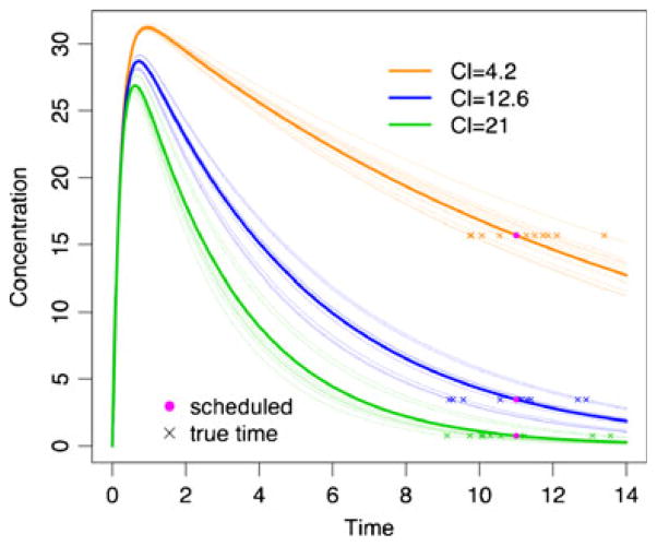
The PK structural component was designed by mimicking a tacrolimus population PK study. Dose 2,000 unit is given every 12 h for 7 days, and the scheduled blood sampling time is just 1 h before each dosing. Our major interest is examining how curvature of PK profile would affect the estimates of PK parameters in the presence of time ME. Different degrees of curvature were investigated, which are governed by CL or elimination rate constant k_e (with V being held at the same value of 60 l). The thick lines in Fig. 5 represent three curvatures with CL =4.2, 12.6 and 21 l h⁻¹ (or k_e =0.07, 0.21 and 0.35 h⁻¹) after a single drug dose, administered orally. Some simulated true time points in the presence of large ME (i.e., σ_u =1.5) along with the corresponding profiles (dotted lines) are also presented around the scheduled time w_ij at 11 h to provide an idea about variability in time ME and curvature. The assumed variance components were σ²=0.02, ω₁₁= ω₂₂=0.04 and ω₁₂=0.02. The data sets were simulated 500 replicates with N =100 subjects for each replicate. All simulations were performed using NONMEM^® [19] and the programming language R version 2.10.0 [20].

Fig. 5.

Profiles as a function of clearance (CL) with V =60 l being held fixed. The thick lines correspond to the data with the scheduled time where CL =4.2, 12.6 and 21 l h⁻¹. Ten simulated true time points in the presence of large time ME (e.g., σ_u =1.5 h) along with the corresponding profiles (dotted lines) are also presented around the scheduled time w_ij at 11 h

Results

Description of figures

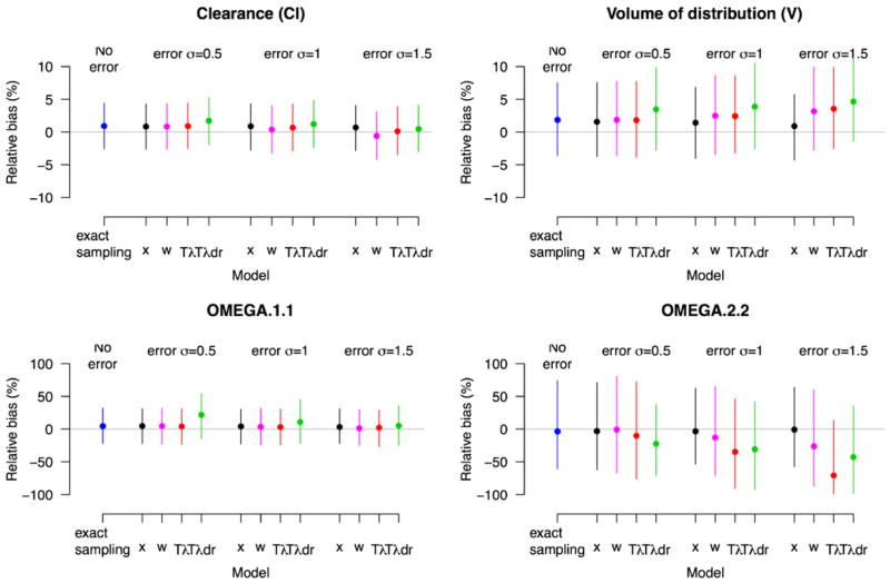
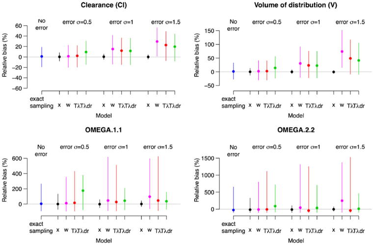
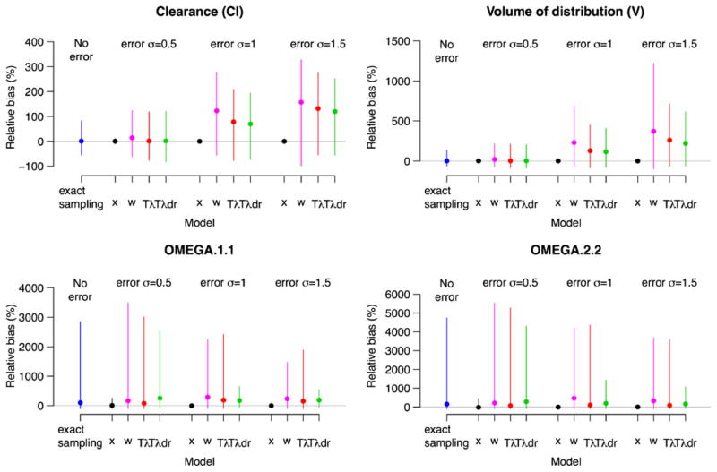
The major simulation results for the cases described in the Section Simulation studies are presented in Figs. 2, 3 and 4. Each figure corresponds to a different true value of CL. The larger the CL with V being fixed, the larger the curvature in the PK profile, demonstrated by the curvature increases from Figs. 2 to 4. The corresponding curvature (thick lines) is shown in Fig. 5 after a single drug dose administered orally. Given our concern relates to bias in parameter estimates due to time ME, the medians of the percent relative biases in parameter estimates along with the 95 percentile intervals are shown in the figures. Also in each figure, the results for population mean estimates of θ = (log CL, log V) are presented in the upper panels with the corresponding variance component in the lower panels. Each panel is divided into four subpanels: “No error” for Case 1 (exact sampling), with the other three labeled “error”, each corresponding to different σ_u. Within the “error” subpanel, Cases 2–5 are presented. Note that other parameters such as λ and σ_u were also estimated by maximum likelihood, but we did not present their estimates, as they are nuisance parameters that are not of interest.

Fig. 2.

The relative bias (%) in PK parameters when clearance is slow (true CL =4.2 l h⁻¹ with V =60 l being held fixed): Case 1 (exact sampling) and Cases 2–5 (x, w, and TBS Tλ and Tλdr) as a function of the size of ME, σ_u =0.5, 1 and 1.5 h. The relative bias (%) is defined by 100 × (θ̂−θ)/θ where θ is the true parameter value and θ̂ is the estimate. The positive values suggest overestimation, while the negative values suggest underestimation. The results for the population means of θ =(log CL, log V) are presented in the upper panels with the corresponding variance component in the lower panels. The solid dots and vertical lines represent the medians and 95 percentiles of the percent relative bias from the simulations. The gray line is drawn to present no bias

Fig. 3.

The relative bias (%) in PK parameters when clearance is slow (true CL =12.6 l h⁻¹ with V =60 l being held fixed): Case 1 (exact sampling) and Cases 2–5 (x, w, and TBS Tλ and Tλdr) as a function of the size of ME, σ_u =0.5, 1 and 1.5 h. The relative bias (%) is defined by 100 × (θ̂−θ)/θ, where θ is the true parameter value and θ̂ is the estimate. The positive values suggest overestimation, while the negative values suggest underestimation. The results for the population means of θ =(log CL, log V) are presented in the upper panels with the corresponding variance component in the lower panels. The solid dots and vertical lines represent the medians and 95 percentiles of the percent relative bias from the simulations. The gray line is drawn to present no bias

Fig. 4.

The relative bias (%) in PK parameters when clearance is slow (true CL=21 l h⁻¹ with V =60 l being held fixed): Case 1 (exact sampling) and Cases 2–5 (x, w, and TBS Tλand Tλdr) as a function of the size of ME, σ_u = 0.5, 1 and 1.5 h. The relative bias (%) is defined by 100 × (θ̂−θ)/θ where θ is the true parameter value and θ̂ is the estimate. The positive values suggest overestimation while the negative values suggest underestimation. The results for the population means of θ =(log CL, log V) are presented in the upper panels with the corresponding variance component in the lower panels. The solid dots and vertical lines represent the medians and 95 percentiles of the percent relative bias from the simulations. The gray line is drawn to present no bias

Major determinants for leading bias

Within each scenario, bias rose dramatically with the increasing order of clearance, which determines the curvature. The most important determinant of bias due to Berkson error in time is the degree of the curvature (nonlinearity) with respect to time in PK profile. The smaller the curvature around sampling times, the smaller the associated bias. Even with large ME, only a small bias results when the curvature is small, as seen in Fig. 2.

Figure 6 displays the second derivatives of the PK mean function with respect to time for: 1) the entire range of one dosing interval (left panel); and 2) a partial range after oral absorption (right panel). If the slope is close to 0 within several hours of the sampling time, such as indicated by the black solid line, the curvature of the corresponding profile can be treated as very small (e.g., CL =4.2 l h⁻¹ for Fig. 2).

Fig. 6.

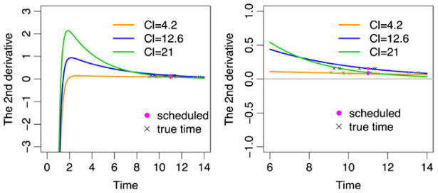
The second derivatives of PK mean functions shown in Fig. 5 (CL =4.2, 12.6, and 21 l h⁻¹) with respect to time after a single dose oral administration. Five simulated true time points in the presence of large time ME (e.g., σ_u =1.5 h) are also presented around the scheduled time w_ij at 11 h. Left panel: the whole time range. Right panel: the time range after oral absorption is approximately finished

Another important determinant is the magnitude of ME. This can be seen by comparing results for each case across different levels of ME within each figure. For fixed effects PK parameter estimates, the larger the ME, the larger the bias, as expected, but the effect of ME is not notable until curvature is substantial. Thus, we conclude that curvature is the most important determinant of bias.

Performance of TBS models (Cases 4 & 5) in comparison with Case 3

Case 4 (Tλ) and Case 5 (Tλdr) correspond to two methods that account for ME in blood sampling time; both performed better than Case 3 (w), especially when curvature and ME were large. There was little difference between Case 4 (Tλ) and Case 5 (Tλdr) in estimating fixed effects PK parameters until ME is substantially large, for which Case 5 (Tλdr) provided a smaller bias compared to Case 4 (Tλ). Regarding estimation of variance components, Case 5 (Tλdr) performed better than Case 4 (Tλ), as well as Case 3 (w), even with small ME.

Design perspective

Comparison of reference Cases 1 and 2 versus Case 3 with small ME

Cases 1 and 2 are reference cases, since both fit the correct model using the true sampling times. The only difference is that the true and scheduled sampling times are the same for Case 1 (exact sampling), while they are different for Case 2 (x). That is, blood samples are drawn exactly at the scheduled times for Case 1, resulting in the same sampling times across all subjects. On the other hand, Case 2 (x) corresponds to the scenario when blood samples are not drawn at the scheduled time, but recorded and used in the analysis; thus, all subjects have different sampling times from design perspective. Case 3 (w) utilizes the scheduled time in its analysis (which is different from the true sampling times). The best results in terms of bias and its variability were obtained with Case 2 (x), while the results for Case 1 (exact sampling) were very comparable with Case 3 (w) when ME is small.

Comparison within Case 2 with varying ME

Under Case 2 (x), the true sampling times increasingly deviate from the scheduled times as ME increases. Results indicate that larger deviations of true sampling time from the scheduled sampling time increased precision, especially for estimating variance components.

Discussion

Berkson ME can lead to substantial bias

Our key finding is that unlike linear regression, Berkson ME in sampling time in PK modeling can indeed lead to bias on the parameter estimators. This bias can be very large depending on curvature of the PK profile and the size of ME.

The curvature is the most important determinant of bias

The major factor leading to bias due to Berkson error in sampling time is the curvature of the PK profiles. This result is intuitive: if the curvature of PK profiles is small, regression on time is roughly linear, which reduces to the Berkson error problem in linear regression. Thus, exactly as Berkson error in linear regression does not affect point estimate bias, regardless of the magnitude of ME, little bias in PK parameter estimates are expected.

For example, the PK profile of tacrolimus has small curvature (CL< 4.2 l h⁻¹), and hence the fixed effects parameters estimates reported in published tacrolimus PK studies are likely not much biased due to time ME, even though a conventional population PK modeling using a scheduled time has been typically performed in those studies. If time ME is anticipated, we strongly recommend— before undertaking a study or PK analysis—making plots such as Figs. 5 or 6, using simulated data sets with a range of PK parameters obtained from the literature or the early stages of clinical trials to assess curvature.

When curvature and time ME are expected to be substantial

When substantial curvature or time ME is expected, conventional population PK modeling using a scheduled time as if true should not be employed, so as to avoid biased estimates. For this case, the methodology of either Case 4 (Tλ) or Case 5 (Tλdr) should be utilized when the focus lies on estimating fixed effects PK parameters. However, the method used in Case 5 (Tλdr) is recommended when precise estimation of random effects is important. Case 5 (Tλdr) provides more power in finding important patient characteristics that alter kinetics, as indicated from narrower 95 percentile intervals of random effects obtained from Case 5 (Tλdr) compared to Case 4 (Tλ).

Design of sampling time: potential gain using exact sampling

The Case 3 (w) method with small ME requires less effort and is convenient. Its design allows taking blood samples at times that deviate slightly from the scheduled ones, while still using the scheduled time in the analysis. The potential gain resulting from taking blood samples exactly at the scheduled time is minimal in the case when ME is small. Conservatively, blood sampling within 30 min of the scheduled time (but without recording this time) would provide reasonable agreement with exact sampling.

Our results indicate that better estimates can be obtained by collecting blood at different time schedules across subjects, confirming the importance of design. Although both Case 1 (exact sampling) and Case 2 (x) used the true times and the correct model in the analysis, Case 2 (x) performed much better than Case 1 (exact sampling), since the Case 2 (x) utilized different time schedules across subjects.

Thus, even when exact sampling at the scheduled time is feasible, it may not be worth the additional effort. Of course, if feasible, exact recording of the sampling times taken at different schedules across all subjects offers the best data.

Dense versus sparse sampling

The focus on studying the effect of time ME on population PK studies with sparse sampling arises from this being the most common form of data generated in routine clinical care. However, it is unclear whether time ME is still problematic in PK studies with dense sampling. To investigate this, simulations with a greater number of sampling time points were conducted. Results indicate that the bias decreased systematically, as the number of samples increased (data not shown).

We conjecture that with frequent sampling, PK profiles would be closer to linear between the sampling time points, which mitigates time ME issues, leading to a general Berkson error problem in linear regression. This also confirms why Wang and Davidian [16] found little bias in their simulation studies that used a dense sampling design. Thus, the increase of sampling frequency reduces bias due to time ME dramatically, and the use of scheduled times is not problematic in PK studies with dense sampling.

Rules of thumb

Based on our results, the following rough guidelines are given for design and analysis in the presence of temporal ME.

1. Little bias expected; conventional PK modeling may be used for:

   • PK data collected with a dense sampling design.

   • Small curvature in PK profile around the scheduled sampling times: when the second derivative of PK curve is plotted as a function of time, the line is approximately linear.

   • Small ME: most true sampling times would lie within approximately 1 hour of the scheduled times.

2. Moderate bias expected; either TBS Tλ or Tλdr should be used:

   • Moderate curvature in PK profile: the line of the second derivative of PK curve no longer appears linear.

   • Moderate ME: most true sampling times would lie within approximately 2 hours of the scheduled times.

3. Large bias expected or precise estimates of random effects needed; TBS Tλdr is preferable:

   • Large curvature in PK profile: the line of the second derivative of PK curve is obviously nonlinear.

   • Large ME: a substantial portion of true sampling times may deviate more than 2 hours from the scheduled times.

   • When precise estimates of random effects are an important aspect of study.

References

- 1.Fukudo M, Yano I, Masuda S, et al. Population pharmacokinetic and pharmacogenomic analysis of tacrolimus in pediatric living-donor liver transplant recipients. Clinical Pharmacology and Therapeutics. 2006;80:331–345. doi: 10.1016/j.clpt.2006.06.008. [DOI] [PubMed] [Google Scholar]
- 2.Han N, Yun H-Y, Hong J-Y, et al. Prediction of the tacrolimus population pharmacokinetic parameters according to CYP3A5 genotype and clinical factors using NONMEM in adult kidney transplant recipients. European Journal of Clinical Pharmacology. 2012:1–11. doi: 10.1007/s00228-012-1296-4. [DOI] [PubMed] [Google Scholar]
- 3.Hamberg A-K, Wadelius M, Lindh JD, et al. A Pharmacometric Model Describing the Relationship Between Warfarin Dose and INR Response With Respect to Variations in CYP2C9, VKORC1, and Age. Clinical Pharmacology and Therapeutics. 2010:727–734. doi: 10.1038/clpt.2010.37. [DOI] [PubMed] [Google Scholar]
- 4.Berkson J. Are There Two Regressions? Journal of the American Statistical Association. 1950;45:164–180. [Google Scholar]
- 5.Carroll RJ, Ruppert D, Stefanski LA, Crainiceanu CM. Measurement Error in Nonlinear Models: A Modern Perspective. 2. Chapman \& Hall/CRC; 2006. [Google Scholar]
- 6.Gustafson P. Measurement Error and Misclassification in Statistics and Epidemiology. Chapman and Hall/CRC; 2003. [Google Scholar]
- 7.Fuller WA. Measurement Error Models. John Wiley \& Sons; New York: 1987. [Google Scholar]
- 8.Wang N, Lin X, Gutierrez RG, Carroll RJ. Bias Analysis and SIMEX Approach in Generalized Linear Mixed Measurement Error Models. Journal of the American Statistical Association. 1998;93:249–261. [Google Scholar]
- 9.Liang H, Wu H, Carroll RJ. The Relationship between Virologic and Immunologic Responses in AIDS Clinical Research Using Mixed-effects Varying-coefficient Models with Measurement Error. Biostatistics (Oxford) 2003;4:297–312. doi: 10.1093/biostatistics/4.2.297. [DOI] [PubMed] [Google Scholar]
- 10.Li E, Zhang D, Davidian M. Conditional Estimation for Generalized Linear Models When Covariates Are Subject-specific Parameters in a Mixed Model for Longitudinal Measurements. Biometrics. 2004;60:1–7. doi: 10.1111/j.0006-341X.2004.00170.x. [DOI] [PMC free article] [PubMed] [Google Scholar]
- 11.Liao JJZ, Schofield TL, Bennett PS. Analyzing Highly Variable Potency Data Using a Linear Mixed-effects Measurement Error Model. Journal of Agricultural, Biological, and Environmental Statistics. 2005;10:148–157. [Google Scholar]
- 12.Liu W, Wu L. Simultaneous Inference for Semiparametric Nonlinear Mixed-Effects Models with Covariate Measurement Errors and Missing Responses. Biometrics. 2007;63:342–350. doi: 10.1111/j.1541-0420.2006.00687.x. [DOI] [PubMed] [Google Scholar]
- 13.Higgins KM, Davidian M, Giltinan DM. ATwo-step Approach to Measurement Error in Time-dependent Covariates in Nonlinear Mixed-effects Models, with Application to IGF-I Pharmacokinetics. Journal of the American Statistical Association. 1997;92:436–448. [Google Scholar]
- 14.Ko H, Davidian M. Correcting for Measurement Error in Individual-level Covariates in Nonlinear Mixed Effects Models. Biometrics. 2000;56:368–375. doi: 10.1111/j.0006-341x.2000.00368.x. [DOI] [PubMed] [Google Scholar]
- 15.Li L, Lin X, Brown MB, et al. A Population Pharmacokinetic Model with Time-dependent Covariates Measured with Errors. Biometrics. 2004;60:451–460. doi: 10.1111/j.0006-341X.2004.00190.x. [DOI] [PubMed] [Google Scholar]
- 16.Wang N, Davidian M. A Note on Covariate Measurement Error in Nonlinear Mixed Effects Models. Biometrika. 1996;83:801–812. [Google Scholar]
- 17.Carroll RJ, Ruppert D. Power Transformations When Fitting Theoretical Models to Data. Journal of the American Statistical Association. 1984;79:321–328. [Google Scholar]
- 18.Rudemo M, Ruppert D, Streibig JC. Random-effect Models in Nonlinear Regression with Applications to Bioassay. Biometrics. 1989;45:349–362. [Google Scholar]
- 19.Beal SL, Sheiner LB, Boeckmann AJ. NONMEM Users Guides. ICON Development Solutions; Ellicott City, MD: 1989. [Google Scholar]
- 20.R Development Core Team. R: a language and environment for statistical computing, Version 2. 5.0. Vienna: R Foundation for Statistical Computing; 2007. [Google Scholar]
Associated Data
This section collects any data citations, data availability statements, or supplementary materials included in this article.