

Abstract
Walking is a commonly available activity to maintain a healthy lifestyle. Accurately tracking and measuring calories expended during walking can improve user feedback and intervention measures. Inertial sensors are a promising measurement tool to achieve this purpose. An important aspect in mapping inertial sensor data to energy expenditure is the question of normalizing across physiological parameters. Common approaches such as weight scaling require validation for each new population. An alternative is to use a hierarchical approach to model subject-specific parameters at one level and cross-subject parameters connected by physiological variables at a higher level. In this paper, we evaluate an inertial sensor-based hierarchical model to measure energy expenditure across a target population. We first determine the optimal movement and physiological features set to represent data. Periodicity based features are more accurate (p<0.1 per subject) when generalizing across populations. Weight is the most accurate parameter (p<0.1 per subject) measured as percentage prediction error. We also compare the hierarchical model with a subject-specific regression model and weight exponent scaled models. Subject-specific models perform significantly better (p<0.1 per subject) than weight exponent scaled models at all exponent scales whereas the hierarchical model performed worse than both. However, using an informed prior from the hierarchical model produces similar errors to using a subject-specific model with large amounts of training data (p<0.1 per subject). The results provide evidence that hierarchical modeling is a promising technique for generalized prediction energy expenditure prediction across a target population in a clinical setting.
Keywords: Accelerometer, Bayesian Linear regression, Gyroscope, Hierarchical Linear Model
1 Introduction
Regular physical activity plays an important role in weight control, reducing risk of cardiovascular disease, type 2 diabetes, some cancers besides improving mental health and bone strength as described by Warburton et al. [2006. Dunn et al. [1999] have shown that an easily available practice for an active lifestyle is to walk regularly. Characterizing energy expenditure from walking would provide a valuable tool in the assessment of activity-based intervention measures.
Over the last decade, commodity-priced kinematic sensors such as accelerometers and gyroscopes have emerged as promising tools for the quantification of calories consumed from human movement. Recent research by Aminian and Najafi [2004], Troiano [2006], Rothney et al. [2007] has focused on combining their small size, low cost, increasingly high precision with pattern recognition techiniques. These techniques rely on learning a data-driven regression map from movement features to a ground truth measure of calorie consumption. Learning regression models from inertial sensors is a well-studied problem as shown by [Vathsangam et al., 2010], [Albinali et al., 2010] and Vathsangam et al. [2011a]. An important issue that arises when learning this map is that the participants of any sample population will exhibit natural variations in weight, height, leg-length, age, sex etc. A successful calorie estimation model must be able to predict calories from movement accurately while accounting for these variations. A natural question to ask is whether it is possible to create a model that allows accurate user-specific modeling while capturing commonalities across users of differing physiological descriptions. If so, what combinations of inertial sensor and physiological features together provide the best descriptors of this model?
In this study, we address the problem of normalizing predictions of energy expenditure across a population when using inertial sensor data to predict calories burnt. We focus on a particular activity: steady-state treadmill walking, because it allows the capture of a repeatable, well-defined and easily quantifiable movement. We use inertial data from a triaxial accelerometer and triaxial gyroscope mounted on the right iliac crest as inputs to describe walking movement and treat the functional mapping of these inputs to energy expenditure as a two-level hierarchical regression problem. Our first goal is to identify the best features to represent movement and physiological parameters as defined by highest prediction accuracy. We then show results comparing the accuracy of the generalized approach with conventional regression models. This study expands on previous work involving hierarchical linear modeling by Vathsangam et al. [2011b]. It differs from the original work in that an in-depth feature study is evaluated for the Hierarchical Linear Model. We also compare our approach to current state of the art speed-based and accelerometer count-based approaches.
2 Related Work
Current techniques for normalizing energy prediction across a population adopt two methodologies. The first family of techniques create isolated user-specific models from each individual’s data. Such models are not likely to be successful for unseen data points of another participant. The second set of techniques learn a general model treating all users as one after normalizing for users based on physical characteristics such as weight or height. For example, a common technique to normalize across participants is to scale energy consumption values by a suitable weight exponent. The participants in the population are then replaced by a single pseudo-participant with weight-scaled energy values. Most common scaling coefficients include a range from 0.6 – 1.0 by Zakeri et al. [2006], the most popular being 0.67 by Neville et al. [1992], 0.75 by Rogers et al. [1995] and 1.0 by Waters and Mulroy [1999], Wyndham et al. [1971] and Pearce et al. [1983]. An issue with weight scaling is determining the appropriate scaling coefficient across a target population. Rogers et al. [1995] showed that scaling coefficients vary across age groups and stages of development in individuals. This means that one has to determine a different scaling coefficient for each new population. Such an approach suppresses the role of individual variances in predicting energy expenditure. Also, Waters and Mulroy [1999] showed that in addition to weight, the effect of other physiological descriptors such as sex, stride length and heart rate also have to be incorporated and it is not clear how scaling based techniques would generalize across these additional parameters.
An important observation to be made when modeling across a population is that the individual participants in the population share common kinematic traits. In the case of energy expenditure from steady-state treadmill walking, all participants share a common property in that steady state walking is cyclical in nature. This individual details of the map from the nature of walk to energy expenditure might vary for each participant. However, similar participants might exhibit similar maps. It might be possible to take advantage of common traits across users to capture a general population model and use it to create better individual models. The challenge is to fuse both the individual and population-based characteristics into a unified framework while maintaining the simplicity of standard regression techniques.
Linear regression can be extended to capture commonalities across a population using a Hierarchical Linear Model (HLM) such as that described by Gelman and Hill [2007]. Given a target population, HLM based techniques use linear models at levels within and across participants. Figure 1 illustrates the principle behind HLMs. At one level we have participant specific models relating inertial sensor features to energy expenditure. At a second level we capture the inter-dependence of different subject-specific models on physiological parameters using a (second) regression model. The advantages of such an approach are many. Using a second level to capture commonalities across subjects allows the separation of the dependence on physiological parameters from participant-specific inertial sensor data. Such an approach also allows flexibility in deciding the right combination of physiological parameters to represent participants. Training this model allows joint modeling of inter-participant information. Most importantly, HLM allows one to generate informed participant-specific models using only higher level information. This is an advantage when limited or no data is available for a new participant. Thus we retain all the benefits of subject-specific monitoring using linear regression while capturing generalizability across populations. Hierarchical Linear Modeling has been successfully used in various biological systems for joint modeling across a population [Gelfand et al., 1990].
Fig. 1.
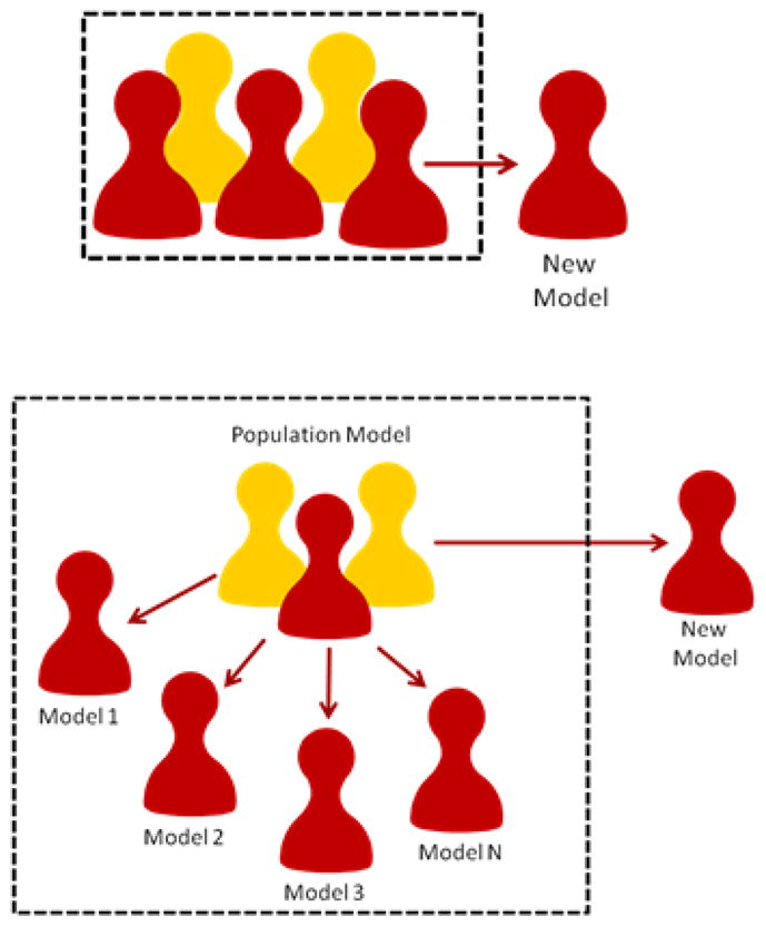
Illustration of the difference between traditional approaches (left) and our approach (right). Rather than treating all subjects as equivalent or developing a separate model per user, we adopt a hierarchical approach to capture common behaviors while retaining individualization.
3 Estimating Energy across a Population
Our goal is to obtain a data-driven functional map from movement features (derived from continuous inertial sensor data) to calories burned (as measured by average V̇O2 consumption). This map must be accurate be obtainable using minimal data from the user. We set this in a regression framework. Consider a D-dimensional input variable x ∈ ℝD of which there are specific data points . The goal of regression is to predict the value of one or more continuous target variables y of which there are corresponding observed values that are related to the input variables by a “best-fit” function f (xn). In this section, we describe a family of techniques for creating individualized regression maps and then extend these techniques normalize these maps across a populating using a Hierarchical Linear Model (HLM).
3.1 Representing Treadmill Walking
Steady state human walk is cyclic in nature [Chang et al., 2004]. We capture this periodicity using a single inertial sensor worn above the iliac crest on the right hip. Sensor data corresponds directly to the accelerations and rotational rates of the hip in the sensor’s local frame of reference. To take advantage of this periodicity, we considered six families of features as described by Tapia et al. [Tapia, 2008]:
Measures of body posture consisting of AC mean across each axis and area under signal
Measures of motion shape consisting of mean of absolute value, total signal vector magnitude, entropy, skewness and kurtosis
Measures of motion variation consisting of variance, coefficient of variation over the absolute value and signal range
Measures of motion spectral content consisting of the normalized Fast Fourier Transform (1024 point FFT) coefficients
Measures of motion energy consisting of total energy, energy in the activity band of 0.3 – 3.5 Hz, energy of low physical activity band of 0.0 – 0.7 Hz and energy in the vigorous physical activity band of 0.71 – 10 Hz in the unnormalized 1024 -point FFTs of raw signals within each epoch
Measures of motion periodicity consisting of mean crossing rate and cepstral coefficients
Any particular category or a combination of these features can be used to represent the input data points .
3.2 Subject-specific energy estimation models with Bayesian Linear Regression
One way to map input features to target values is to use a separate linear regression model for each participant. We adopt a Bayesian approach through Bayesian Linear Regression (BLR). The approach is similar to our earlier work in predicting energy expenditure [Vathsangam et al., 2010]. Figure 2 represents a graphical model based plate representation of the conventional BLR technique.
Fig. 2.
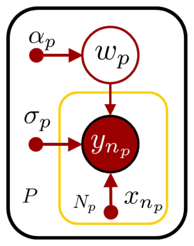
Illustration of individualized energy prediction model. Training the model is equivalent to finding optimal w to maximize data likelihood. A distribution is assumed over w: w ~
 (w: 0, α−1I). α is a hyper-parameter.
In the context of energy prediction, for a given person p, with input feature data set and target energy values :
| (1) |
where ε is a noise parameter and wp = (w0p, …, wM−1p)T are the model weights. Training the model is equivalent to learning the weights wp and the noise parameters σp. Using the properties of Gaussian distributions, we have
| (2) |
Bayesian Linear Regression (BLR) Bishop [2006a] adopts a Bayesian approach to linear regression by introducing a prior probability distribution over wp. We choose a Gaussian prior, p(wp) =
(wp; 0, α
−1I)over the model parameters wp. The optimal prediction for a new data point is given by the predictive distribution:
| (3) |
| (4) |
| (5) |
| (6) |
Model parameters are estimated by finding the best α and σp to maximize the evidence function, finding the best parameters ŵ to maximize the likelihood given a fixed α and σp alternately until convergence. This technique provides a subject-specific BLR model that can be trained and used for each participant separately.
3.3 Generalizing Energy Estimation Models with Hierarchical Regression
3.3.1 Model description
We build on the individualized model to obtain an HLM incorporating physiological features. Consider a test population consisting of P participants. For each participant p, let there be Np data points collected, consisting of the energy values Yp = {y1p, y2p, …, yNp} and D-dimensional feature inputs Xp = {x1p, x2p, …, xNp} as detailed in Sec. 4.2. We denote Y = {Y1, Y2, …, YP} and X = {X1, X2, …, XP} to be complete set of training data for all participants. Let each participant have physiological features determined by Physp and the complete set be These include parameters such as height, weight and age (with a constant term for bias). We model top-down dependence of wp on each participant’s physiological features Physp through a universal weight parameter k. Each wp in turn influences energy predictions ynp for an input xnp. Figure 3 illustrates the plate representation of the hierarchical model. Similar to Sec. 3.2, each output energy value, ynp is linearly dependent on input xnp. This can be expressed as:
| (7) |
| (8) |
Fig. 3.
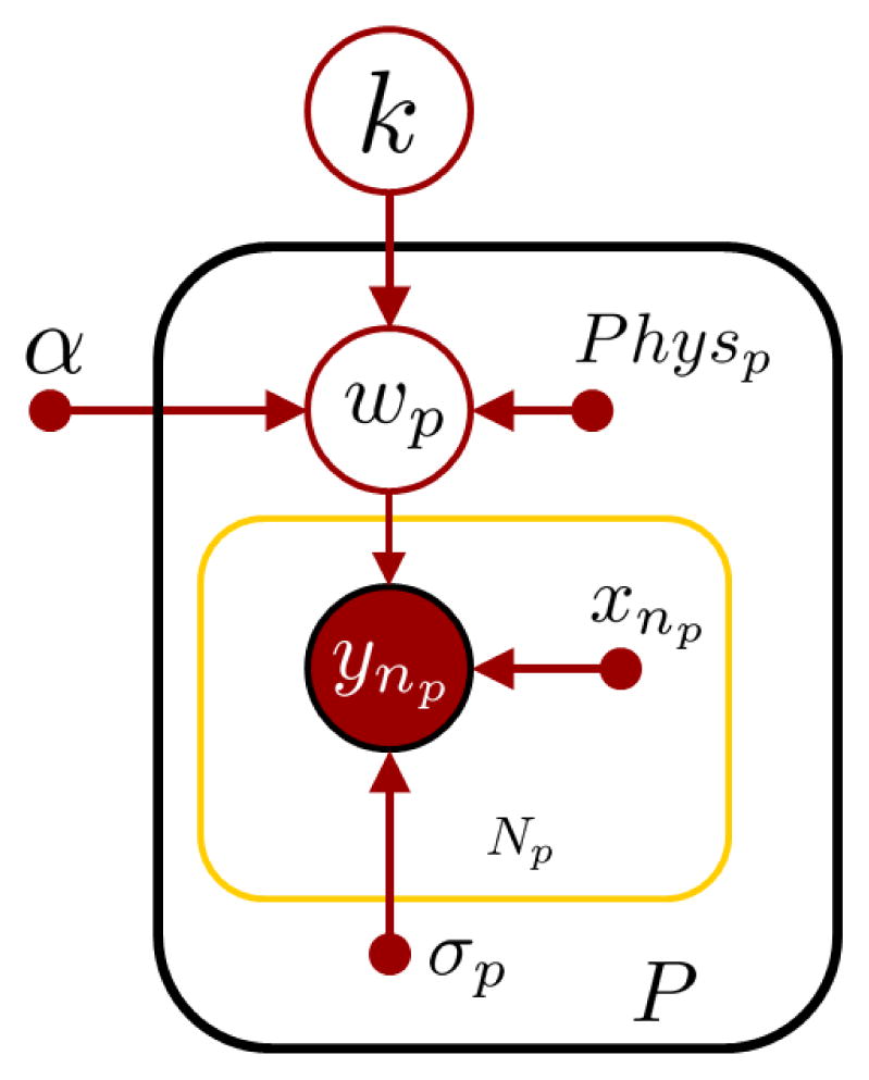
Illustration of generalized model for energy expenditure prediction for P people and Np training points per person. Each person has a subject-specific weight wp that is influenced by physiological parameters such as height, weight and age through k and in turn influences energy prediction given an input point xnp.
Our model differs from the BLR case in that, we assume that the prior distribution overwp is not uninformative but has a linear dependence on k and Physp:
| (9) |
Both wp and k are hidden variables which need to be estimated from data. Variable k is also not a point estimate but has a prior distribution k ~
(k; 0, σ
−2I). Each wp is now an informative prior dependent on the person’s physiological features Physp through k. We denote
Training the multilevel model is equivalent to learning individual wp’s, the overall parameter k as well as the noise parameters , α and σ. The HLM combines P personal regression models in two ways. First, the local regression coefficients wp determine energy values for each person. Second, the different coefficients are connected through the population-level model parameter k. Intuitively, the HLM captures the inherent similarity in walking across different people while accounting for individual walking styles and energy consumption.
3.3.2 Likelihood evaluation
We aim to find the optimal parameters that maximize the likelihood of each energy prediction ynp for each person p, given the input data points xnp and the physiological features Physp. This likelihood can be written as:
| (10) |
| (11) |
| (12) |
p(W|X, PHYS) can be expressed in terms of hidden variable k as:
| (13) |
From the graphical model in Fig. 3, the probabilities p(Y|W, X, PHYS) and p(W|X, k, PHYS) can be broken down into individual distributions as:
From the model graph, we can infer wp ⫫ Xp|k, Physp, ynp ⫫ Physp|xnp, wp and k ⫫ PhyspXp. Thus:
| (14) |
| (15) |
| (16) |
Substituting Eqs. 14, 15 and 16 into Eqs. 12 and 13, we have:
| (17) |
The pair of equations represented by [17] represent the likelihood of the observations Y given physiological features PHY and inputs X. Maximizing the log - likelihood,
 = log l is equivalent to finding the optimal wp,k and respective noise parameters that maximize these equations. Of particular interest is parameter k ∈ ℝD which helps generate a person dependent weight wp given only the physiological parameters. The probabilities p(ynp |xnp,
wp) and p(wp|k,
Physp) are defined by Eqs. 8 and 9 respectively. For the class of exponential distributions in the absence of prior information, there is no closed form solution for
and k. Hence approximation techniques are required. Table 1 summarizes the terms used in our model.
= log l is equivalent to finding the optimal wp,k and respective noise parameters that maximize these equations. Of particular interest is parameter k ∈ ℝD which helps generate a person dependent weight wp given only the physiological parameters. The probabilities p(ynp |xnp,
wp) and p(wp|k,
Physp) are defined by Eqs. 8 and 9 respectively. For the class of exponential distributions in the absence of prior information, there is no closed form solution for
and k. Hence approximation techniques are required. Table 1 summarizes the terms used in our model.
Table 1.
Glossary of Terms
| Term | Description | Dim |
|---|---|---|
| xnp | nth input point for person p | 1 × D |
| ynp | nth target V̇O2 for person p | 1 × 1 |
| wp | Weight parameter for person p | 1 × D |
| k | Population weight parameter | 1 × D |
| Physp | Physiological features | 1 × (M + 1) |
| σp | Noise parameter for person p | 1 × 1 |
| σ | Prior variance for k | 1 × 1 |
| α | Variance for wp | 1 × 1 |
| Np | Number of data points for person p | − |
| Xp | Collection of input data for person p | Np × D |
| Yp | Collection of V̇O2 values for person p | Np × 1 |
| X | Collection of all input data points | P × Np × D |
| Y | Collection of all V̇O2 values | P × Np × 1 |
| PHY | Collection of all physiological values | P × (M + 1) × 1 |
3.3.3 Algorithm description
We propose an EM like algorithm Bishop [2006b] to learn the parameters
and k. Our original aim was to maximize the likelihood
= log p(Y|X,
PHY). We approximate the likelihood term to incorporate the maximum a posteriori estimates of individual weights wp denoted by ŵp. Each ŵp is now a point estimate assumed to be known and can be interpreted as a parameter that has to be optimized. From Eq. 9, the MAP estimate corresponds to the mean of each wp. The modified algorithm maximizes the incomplete log likelihood log p(Y|Ŵ,
X,
PHY). It does so by maximizing the expected complete log likelihood 〈log p(Y,
Z|Ŵ,
X,
PHY)〉. This expectation is written as:
We treat k as a hidden variable that needs to be estimated and hence Z = k. Correspondingly, we have the following steps:
Initialization Initialize ŵp, σp, α to appropriate values. An appropriate initialization condition is one obtained using least squares estimates.
E step
Evaluate . For this, we take advantage of the linear dependence of each person’s weight vector ŵp given their physiological features Physp through k. This means we have a data set of P target ŵp’s and their corresponding input variables Physp’s. We can thus frame a regression problem from a person’s physiological parameter variable Phys to a weight variable ŵ (of which there are P examples) through k. Assuming that k ∈ ℝD and no covariance terms, we frame D separate linear regression problems. The mth regression problem, maps the physiological features to the mth component of ŵ through the mth component of k. Thus we have D separate linear regression problems mapping physiological features Physp to wEM through k in a component-wise manner. We solve each of these regression problems in a BLR framework similar to that described in Sec. 3.2 to obtain a mean and variance measure for k.
M step
Maximize likelihood of the data set given k. This corresponds to re-estimating parameters using the current value of k. The learned k from the E-step is used to estimate individual ŵp’s given their physiological features Physp. From the linear relationship as defined by Eq. 9, we have:
| (18) |
We use this estimate as initial conditions and maximize the likelihood of the data set. Given k (which is fixed after the E-step), this is equivalent to maximizing individual likelihoods of each of the participants. Maximizing the individual likelihoods is the same as finding the optimal wp given Np data pairs . This is equivalent to solving P individual Bayesian Linear Regression problems with the initial conditions of wp’s as defined above and finding the optimal wp’s.
Evaluate log likelihood
The total log likelihood is the sum of the P individual log likelihoods found from the M step. We check for convergence of log likelihood and if not, repeat the E and M steps again. Using this algorithm we learn a generalized energy prediction model that maps physiological features to subject specific weights wp and uses these weights to predict energy expenditure for each subject.
4 Methods
4.1 Hardware
Human movement was captured using a modified Sparkfun 6DoF Inertial Measurement Unit (IMU) [2009] worn on the right iliac crest. The sensor provided 6 sensor streams conveying triaxial acceleration through a Freescale [2008] MMA7260Q triaxial accelerometer from and triaxial rotational rates through 2 Invensense [2006] IDG300 gyroscopes allowing translational and rotational motion capture in all three planes –sagittal, frontal and transverse. The accelerometer was set at ±2g range. Data were sampled at 100 Hz and transmitted via Bluetooth (RN-41 Bluetooth module) to a nearby PC. Additionally, activity patterns in the form of accelerometer counts as generated from a single Actigraph GT1M (10 second epochs) were recorded. The GT1M was mounted firmly on top of the IMU with the X and Y axes of both sensors aligned as close as possible. Figure 4a illustrates the hardware setup used for collecting data.
Fig. 4.
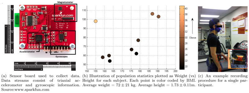
Illustration of hardware, ground truth collection and population statistics
(a) Sensor board used to collect data. (b) Illustration of population statistics plotted as Weight (vs) (c) An example recording Data streams consist of triaxial ac- Height for each subject. Each point is color coded by BMI. procedure for a single par-celerometer and gyroscopic information. Average weight = 72 ± 21 kg. Average height = 1.73 ± 0.11m. ticipant. Source:www.sparkfun.com
4.2 Data collection
Nine healthy adults (Five men, four women) participated in the study. Height and weight of each participant were recorded using a Healthometer balance beam scale. Figure 4b illustrates participant statistics using a Weight (vs) Height graph. Each point is color coded by Body Mass Index (BMI). Informed written consent was obtained from participants and the study was approved by the Institutional Review Board, University of Southern California. Participants had average weight = 72±21 kg and average height = 1.73 ± 0.11 m.
Rate of oxygen consumption (V̇O2, ml/min) as measured using the MedGraphics Cardio II metabolic system with BreezeSuite v6.1B (Medical Graphics Corporation) was the representation of energy expenditure. Before each test, the flow meter was calibrated against a 3.0 L syringe and the system was calibrated against O2 and CO2 gases of known concentration. This system outputs data at the frequency of every breath. Figure 4c illustrates a typical recording procedure. Each participant was asked to walk at 5 speeds (2.5, 2.8, 3.0, 3.3, and 3.5 mph) on a motorized treadmill for 7 minutes of recording time per speed. At each speed transition, V̇O2 readings were allowed to stabilize for 2 minutes prior to the start of data collection. Speeds were chosen based on the Compendium of Physical Activities [Ainsworth et al., 2000].
4.3 Data Preparation
Each sensor stream from the IMU was passed through a low pass filter with 3dB cutoff at 20 Hz. The cutoff frequency was chosen keeping in mind that everyday activities fall in the frequency range of 0.1–10 Hz as was shown by Bao and Intille [2004]. Each of the 7 minute streams from the IMU were divided into 10 second intervals or epochs. The 10 second interval was chosen based on previous successful implementations by Vathsangam et al. [2010]. Each subject’s data consists of roughly 210 data points. Within each epoch, feature vectors were extracted from each sensor stream as explained in Sec. 3.1. A combination of these features represent the input points xnp as described in Sec. 3.3. When it was required to extract an FFT over a signal, the Fourier coefficients corresponding to frequencies greater than 10 Hz were discarded. All features were calculated for both the accelerometer and gyroscope and for each axis within each. Data for each user was thus a set of epochs each containing 6-dimensional raw data and the average rate of oxygen consumption (V̇O2) for that epoch. These represent per-user data while walking at five different speeds.
4.4 Reference Equations for Comparison
In order to compare our approach with current state-of-the-art techniques, a speed based calorie prediction obtained from The ACSM [2010] Exercise Guidelines and an Actigraph count-based 2-regression model by Crouter et al. [2006] were also calculated on the corresponding recorded speeds and synchronized Actigraph data respectively. The ACSM Exercise Guidelines provide a means to estimate calories burnt from the speed of walk as:
Crouter et al. [2006] provides a method to convert 10 second epoch based accelerometer counts to calories consumed as:
Errors for all models were measured as least-squared error from the ground truth output from the metabolic cart.
5 Results and Discussion
This section provides a comparative analysis of prediction accuracy based on different models. Models were varied across two axes. First, a comparative feature study was performed to identify the best feature space for the Hierarchical Linear Model and the subject-specific regression model. The best feature space was defined as that which resulted in the least percentage prediction errors across participants. Second, given the optimal feature space the Hierarchical Linear Model was compared with subject-specific and weight-scaled approaches to determine relative accuracies. Unless otherwise stated, all results were statistically significant (p<0.1 per participant).
5.1 Feature Study
5.1.1 Choosing Optimal Movement Features
Given candidate feature families as described in Sec. 3.1, our first study focused on determining the best feature space to represent human movement. Once again, the best candidate was determined as that which minimized the V̇O2 prediction error. Figure 5 summarizes the results. In each run, data from one participant p was selected. 60% of this data was randomly partitioned into training data, the remaining constituting test data. Five different feature families were extracted from the epochs corresponding to the training data. Five different subject-specific models (shown in yellow) for each of the feature families using participant p’s training data alone. Energy predictions were made for participant p’s test data. Simultaneously, five different HLMs (shown in red) were trained using all data from the remaining P −1 participants and energy predictions were made for participant p’s test data. For reference, speed-based (shown in black) and count-based (shown in gray) V̇O2 calculation techniques were also implemented on the same test data. This was repeated five times for different randomly partitioned training and test data and a per-participant error was calculated. This procedure was repeated for each participant p and errors were averaged across all participants.
Fig. 5.

Comparison of errors obtained from different feature spaces using the HLM (red) and subject-specific models averaged across all participants (yellow). The 1024 point FFT produced the least error in both the subject-specific model and HLM. Errors from the HLM were roughly twice that of the subject-specific regression models. The second lowest errors in the subject-specific model cases were obtained using motion shape as a feature. Corresponding second lowest errors in the HLM cases were obtained when using motion periodicity as a feature. Features that constitute motion shape and motion variation vary across experiment sessions and lead to poor generalizations. Features that derive periodicity are more reliable across a population.
The 1024 point FFT produced the least error in both the subject-specific model and HLM. Errors from the HLM were roughly twice that of the subject-specific regression models. Subject-specific regression models performed better than speed or count based techniques. An interesting observation is that while the second lowest errors in the subject-specific model cases were obtained using motion shape as a feature, the corresponding second lowest errors in the HLM cases were obtained when using motion periodicity as a feature. Features that constitute motion shape and motion variation vary across experiment sessions. These feature values can change with slight changes in orientation, location of sensor, differing walking styles between sessions in addition to natural variations across participants. On the other hand, since steady-state walking is a cyclical activity, features that derive this periodicity are more reliable across a population. The 1024 point FFT is a case of fine-grained tracking of periodicity. This is the primary reason why periodicity based features perform better than motion shape or motion variation based features. Given that it produced the lowest error rates, in both subject-specific models and HLMs the 1024 point FFT was used as the only feature space to represent human movement for the remainder of this study.
5.1.2 Choosing the Single-best Optimal Physiological Feature
Given the 1024 point FFT transform as the optimal feature set to represent movement, the second study examined the best set of physiological features that minimized energy expenditure prediction errors. The features used were Height, Weight, BMI, Age and all features combined. We did not consider combinations of features because the small size of our population made the algorithm prone to overfitting. Maximum errors were obtained when only height was used as a feature vector. The best individual physiological feature for this population was weight. Combining weight and height only marginally improved performance and adding age degraded performance. Based on the above results, it was decided to use weight as the only physiological feature. Figure 6 illustrates the errors obtained. With these results in mind, the optimal feature space was chosen to be the 1024 point FFT at the individual level and weight only at the population level.
Fig. 6.

Illustration of prediction errors (expressed as percentage of ground truth) with different combinations of physical parameters. Maximum errors were obtained when only height was used as a feature vector. Among features chosen weight is the single best physiological features to estimate k.
5.2 Algorithm Comparison
5.2.1 Comparison with Subject-specific Modeling
Given the optimal feature space, an important question is how the HLM compares with subject-specific models. Fig. 7 illustrates the relative errors obtained when an HLM (shown in red) trained using data from P −1 people is compared with a subject-specific model for the pth person with varying training data (shown in yellow) averaged across all participants. The testing methodology was similar to that described in Section 5.1.1 except that the feature set was kept constant and the percentage of training data was varied. For reference, speed based and accelerometer count based calorie determination techniques also shown. The HLM showed the same accuracy at all percentages of training data and hence only one bar is shown. The HLM showed comparable errors to subject specific models with 10% of training data used. With more training data, subject specific models outperformed the HLM and speed/count based approaches. The availability of more training data allows stronger modeling capability of subject-specific models. An HLM still showed the same level of performance as a subject-specific model with small amounts of data. Hence, in cases where no data from a subject is available, using an HLM might be a preferable option to predict calories burnt. With large amounts of data, a subject-specific model with large amounts of data would perform better than both the HLM and speed/accelerometer based approaches described. It can be shown that predictions from a BLR model (used in estimating k’s) approach the ideal value with increasing large amounts of training data. Hence it is expected that as the size of the target population is expanded, the HLM will perform competitively with the subject-specific approach.
Fig. 7.

Comparison of errors obtained from the HLM (red) with individualized subject-specific models averaged across all participants (yellow). The generalized model showed comparable errors to subject-specific models with 10% of training data. With more training data, subject-specific models outperformed the generalized model and previous speed or accelerometer based approaches.
5.2.2 Utilization of HLM as an Informative Prior
Given the superior performance of subject-specific models, this section of the study explores whether a hybrid approach utilizing both an HLM and a subject-specific model could be used to produce even more accurate results. This can be achieved by combining the weights obtained using the generalized model with limited training data to equal or improve model prediction accuracy. Such an approach would be beneficial because it offers the potential of using less training data for training subject-specific models. Given the learned k, from a HLM, one can predict the subject specific weight ŵp for an unknown subject using Eq. 18. One can then train a subject-specific model with this ŵp as an informative initial condition and limited subject-specific data. Fig. 8 illustrates percentage errors obtained with varying amounts of training data. Training a model with an informative prior that was learned from the generalized model (red) showed lower errors when compared with cases where an uninformative prior was used (yellow). This was most pronounced when small amounts of training data are used (p<0.1 per subject). It can also be seen from the figure that using an informative prior with small amounts of training data showed comparable errors to training with no an uninformative prior and substantial training data. The use of an informative prior also showed higher accuracy than existing speed-based or accelerometer based techniques. This approach suggests that while the HLM by itself produces higher errors than a subject-specific model, the lowest errors can be obtained by using the k from the model to obtain a subject specific weight ŵp and using this ŵp as an informative prior with small amounts of training data from the participant.
Fig. 8.

Illustration of the effect of adding a small amount of subject-specific training data to the HLM. An informative prior from physiological features is used to train a subject-specific model, shown in red. For comparison, a subject-specific model (shown in yellow) with an uninformative prior is also trained. Using an HLM with initial conditions along with a small percentage of training data produced similar errors to using a subject-specific model with large amounts of training data (p<0.1 per subject).
5.2.3 Sources of Model Inaccuracies
Figure 9 illustrates the relative predictive capacities of the HLM and subject-specific model as applied to one participant. It can be seen that while the HLM made as good V̇O2 predictions as the subject-specific model in the middle energy range, the model broke down when predicting lower or higher energy ranges. This can be understood as follows, the HLM has to simultaneously fit model parameters across participants and within each participant. Most participants’ walking styles exhibit the most variation at edges of the walking speed range due to natural physiological differences such as weight, height and leg-length. The generalized model has to tradeoff between overall accuracy and subject-specific accuracy. Therefore, the parameters are optimized over the most similar looking input points which occur in the middle ranges of speeds of each participant. This is typical of the bias-variance tradeoff involved in learning such models.
Fig. 9.

Illustration of the predicted values versus ground truth using both generalized algorithms (red) and subject-specific algorithms (blue) for a single participant. Similar plots exist for other participants. HLMs perform poorly in the end regions. This could be because the parameters are optimized over the most similar looking input points. These occur in the middle ranges of speeds of each participant.
5.2.4 Comparison with Weight-scaled Models
As was described in Section 2, current normalizing approaches model weight dependence by using power law scaling. V̇O2 values are scaled by a weight exponent of the form Ws. All participants are considered to represent a single data set and each V̇O2 value is scaled by a suitable weight exponent Ws as . This section of the study focused on how the HLM and subject-specific models compare against such scaling based approaches. The unified data set was divided into training and testing data and regression models were trained. This was repeated for different randomly sampled data and percentages of training and testing data. Various exponent coefficients in the range 0.6 < s < 1.6 were used in increments of 0.1 and percentage errors (as defined in previous section) were recorded. Thus for different combinations of training data and exponent coefficients, we have an error surface. Fig. 10a shows the surface as seen from above. This represents a color plot of errors for various training percentage-exponent coefficient combinations. Lowest errors (≈6.5%) were seen with an exponent coefficient of 0.7 – 1.0 and a large percentage of training data (> 50%). This exponent coefficient value corresponded to previous research indicating that the optimal value is approximately 0.65 – 1.0.
Fig. 10.

Comparison of HLM and subject-specific models with weight-scaled linear approaches. V̇O2 values are scaled by a weight exponent Ws where 0.6 < s < 1.6 and probabilistic linear models are trained, these are compared against the subject-specific and generalized model described in this study.
Fig. 10b illustrates a comparative performance between power law scaled approaches, generalized model and subject-specific model based approaches for different power co-efficients at all training percentages. Subject-specific models outperformed weight exponent scaled models irrespective of exponent. This is because each subject-specific model used training data only from that particular participant. This would naturally result in a better fit than any form of weight scaling across all participants. Generalized models performed worse than subject-specific or weight exponent scaled models but performed better than either when a small amount of training data was used.
6 Conclusion
Accurately tracking and measuring calories burned from walking provides a valuable tool in designing effective intervention measures. The last decade has seen the emergence of inertial sensors to detect, characterize and quantify physical activity. An issue with using inertial sensor data to estimate energy expenditure is how data can be normalized across varying physiological features such as height, weight, age etc. Common approaches such as weight scaling require validation across each new target population. An alternative is to extend the capability of standard linear regression through Hierarchical Linear Modeling (HLM). At one level we have participant specific models relating inertial sensor features to energy expenditure. At a second level we capture the inter-dependence of participant-specific models on physiological features using a second regression model. Our contributions are summarized as:
Flexibility in modeling physiological and feature parameters
HLMs allow flexibility in incorporating features both at the physiological and sensor modeling level. By differentiating these features at multiple levels, one can easily switch, add or remove various combinations and examine their effects on prediction accuracy. In our study, weight was the single best physiological feature and a 1024-point FFT was the best feature for description of movement.
Accurate models with sparse data
In many studies across a large population, researchers often have to deal with inadequate or unequal amounts of data from participants. Capturing inter-participant dependencies through a higher level of modeling allows one to effectively “transfer” model information from those participants for whom extensive data are available to those where only limited data are available. Our implementation demonstrated the effectiveness of using the HLM to obtain an informative initial condition to further train individual models. Despite having access to sparse data, using an informative initial condition produced similar errors to a subject-specific model with large training data.
Comparison with subject-specific and weight-scaled modeling
The generalized model showed similar errors to subject-specific models with 10% of training data used. Subject-specific models performed better than weight exponent scaled models for all exponent scales. An important insight was that generalized models showed competitive prediction accuracies with the subject-specific model in the middle energy range for each subject but broke down when predicting for lower or higher energy ranges. This is most likely because most subjects exhibit similar walking patterns in the mid-speed ranges.
7 Future Work
We plan to expand our work in a number of directions. The most important extension is to test our algorithm across a much larger population and more comprehensive set of activities. Testing across a larger population will also allow a comparison between the effects of other physiological features such as height, stride length and sex on prediction accuracies. We also aim to test the algorithm in free-living conditions across common activities such as walking, sitting and standing. Finally, we plan to compare other approaches that learn the parameters k and wp, including Gibbs-sampling and variational approximations.
Acknowledgments
This work was supported in part by Qualcomm, Nokia, NSF (CCR-0120778) as part of the Center for Embedded Networked Sensing (CENS), and the USC Comprehensive NCMHD Research Center of Excellence (P60 MD 002254). Support for H. Vathsangam was provided by the USC Annenberg Doctoral fellowship program. The authors would like to thank David Erceg of the Division of Biokinesiology and Physical Therapy, USC, for his invaluable support and guidance.
Contributor Information
Harshvardhan Vathsangam, Email: vathsang@usc.edu, Dept. of Computer Science, University of Southern California, Los Angeles, CA - 90007.
B. Adar Emken, Email: emken@usc.edu, Dept. of Preventive Medicine, University of Southern California, Los Angeles, CA - 90007.
E. Todd Schroeder, Email: eschroed@usc.edu, Division of Kinesiology, University of Southern California, Los Angeles, CA - 90007.
Donna Spruijt-Metz, Email: dmetz@usc.edu, Dept. of Preventive Medicine, University of Southern California, Los Angeles, CA - 90007.
Gaurav S. Sukhatme, Email: gaurav@usc.edu, Dept. of Computer Science, University of Southern California, Los Angeles, CA - 90007
References
- 6D oF Inertial Measurement Unit Datasheet. Technical report. Sparkfun Electronics; 2009. URL http://www.sparkfun.com/products/8454. [Google Scholar]
- ACSM. ACSM’s Guidelines for Exercise Testing and Prescription. American College of Sports Medicine; 2010. [DOI] [PubMed] [Google Scholar]
- Ainsworth BE, Haskell WL, Whitt MC, Swartz AM, Strath SJ, O’Brien WL, Bassett DR, Jr, Schmitz KH, Emplaincourt PO, Jacobs DR, Leon AS. Compendium of physical activities: classification of energy costs of human physical activities. Med & Sci in Sports & Exer. 2000;32:S498–S516. doi: 10.1097/00005768-200009001-00009. [DOI] [PubMed] [Google Scholar]
- Albinali Fahd, Intille Stephen, Haskell William, Rosenberger Mary. Using wearable activity type detection to improve physical activity energy expenditure estimation. 12th conference on Ubiquitous Computing; 2010. [DOI] [PMC free article] [PubMed] [Google Scholar]
- Aminian Kamiar, Najafi Bijan. Capturing human motion using body-fixed sensors: outdoor measurement and clinical applications. Computer Animation and Virtual Worlds. 2004;15(2):79–94. [Google Scholar]
- Bao Ling, Intille Stephen S. Activity Recognition from User-Annotated Acceleration Data. In: Alois, editor. PERVASIVE. Massachusetts Institute of Technology, Springer-Verlag GmbH; Apr, 2004. pp. 1–17. [Google Scholar]
- Bishop Christopher M. Pattern Recognition and Machine Learning. Vol. 3.3. Springer; 2006a. pp. 152–156. [Google Scholar]
- Bishop Christopher M. Pattern Recognition and Machine Learning. Vol. 9.4. Springer; 2006b. pp. 450–454. [Google Scholar]
- Chang C, Ansari R, Khokhar AA. Efficient tracking of cyclic human motion by component motion. 12. 2004. pp. 941–944. [Google Scholar]
- Crouter Scott E, Clowers Kurt G, Bassett David R. A novel method for using accelerometer data to predict energy expenditure. J Appl Physiol. 2006 Apr;100(4):1324–1331. doi: 10.1152/japplphysiol.00818.2005. [DOI] [PubMed] [Google Scholar]
- Dunn AL, Marcus BH, Kampert JB, Garcia ME, Kohl HW, III, Blair SB. Comparison of Lifestyle and Structured Interventions to Increase Physical Activity and Cardiorespiratory Fitness: A Randomized Trial. JAMA. 1999;281:327–334. doi: 10.1001/jama.281.4.327. [DOI] [PubMed] [Google Scholar]
- Freescale. 1.5g – 6g three axis low-g micromachined accelerometer. Technical report. 2008 URL http://www.freescale.com/files/sensors/doc/data_sheet/MMA7260QT.pdf.
- Gelfand AE, Hills SE, Racine-Poon A, Smith AFM. Illustration of bayesian inference in normal data models using gibbs sampling. Journal of the American Statistical Association. 1990;85:972–985. [Google Scholar]
- Gelman Andrew, Hill Jennifer. Data Analysis Using Regression and Multilevel/Hierarchical Models. Cambridge University Press; 2007. [Google Scholar]
- Invensense. Integrated dual-axis gyro - idg 300. Technical report. 2006 URL http://www.sparkfun.com/datasheets/Components/IDG-300_Datasheet.pdf.
- Neville AM, Ramsbottom R, Williams C. Scaling physiological measurements for individuals of different body size. Eur J Appl Physiol Occup Physiol. 1992;65(2):110–7. doi: 10.1007/BF00705066. [DOI] [PubMed] [Google Scholar]
- Pearce M, Cunningham D, Donner A, Rechnitzer P, Fullerton G, Howard J. Energy cost of treadmill and floor walking at self-selected paces. European Journal of Applied Physiology and Occupational Physiology. 1983;52:115–119. doi: 10.1007/BF00429037. [DOI] [PubMed] [Google Scholar]
- Rogers DM, Olson BL, Wilmore JH. Scaling for the vo_2-to-body size relationship among children and adults. J Appl Physiol. 1995;79(3):958–967. doi: 10.1152/jappl.1995.79.3.958. [DOI] [PubMed] [Google Scholar]
- Rothney Megan P, Neumann Megan, Beziat Ashley, Chen Kong Y. An artificial neural network model of energy expenditure using nonintegrated acceleration signals. J Appl Physiol. 2007;103(4):1419–1427. doi: 10.1152/japplphysiol.00429.2007. URL http://jap.physiology.org/cgi/content/abstract/103/4/1419. [DOI] [PubMed] [Google Scholar]
- Tapia Munguia. PhD thesis. Massachusetts Institute of Technology. Dept. of Architecture. Program in Media Arts and Sciences; 2008. Using machine learning for real-time activity recognition and estimation of energy expenditure. [Google Scholar]
- Troiano Richard P. Translating accelerometer counts into energy expenditure: advancing the quest. J Appl Physiol. 2006 Apr;100(4):1107–1108. doi: 10.1152/japplphysiol.01577.2005. [DOI] [PubMed] [Google Scholar]
- Vathsangam H, Emken A, Schroeder ET, Spruijt-Metz D, Sukhatme GS. Determining Energy Expenditure From Treadmill Walking Using Hip-Worn Inertial Sensors: An Experimental Study. IEEE Transactions on Biomedical Engineering. 2011a Oct;58(10):2804 –2815. doi: 10.1109/TBME.2011.2159840. [DOI] [PMC free article] [PubMed] [Google Scholar]
- Vathsangam Harshvardhan, Emken Adar, Todd Schroeder E, Spruijt-Metz Donna, Sukhatme Gaurav S. Towards a Generalized Regression Model for On-body Energy Prediction from Treadmill Walking. 5th International ICST Conference on Pervasive Computing Technologies for Healthcare; 2011b. [Google Scholar]
- Vathsangam Harshvardhan, Emken Adar, Spruijt-Metz Donna, Schroeder Todd E, Sukhatme Gaurav S. Energy Estimation of Treadmill Walking using On-body Accelerometers and Gyroscopes. EMBC. 2010 doi: 10.1109/IEMBS.2010.5627365. [DOI] [PubMed] [Google Scholar]
- Warburton Darren ER, Whitney Crystal, Shannon SD. Bredin. Health Benefits of Physical Activity. CMAJ. 2006:174. doi: 10.1503/cmaj.051351. [DOI] [PMC free article] [PubMed]
- Waters Robert L, Mulroy Sara. The energy expenditure of normal and pathologic gait. Gait & Posture. 1999;9(3):207 – 231. doi: 10.1016/s0966-6362(99)00009-0. [DOI] [PubMed] [Google Scholar]
- Wyndham C, van der Walt W, van Rensburg A, Rogers G, Strydom N. The influence of body weight on energy expenditure during walking on a road and on a treadmill. European Journal of Applied Physiology and Occupational Physiology. 1971;29:285–292. doi: 10.1007/BF00697731. [DOI] [PubMed] [Google Scholar]
- Zakeri I, Puyau MR, Adolph AL, Vohra FA, Butte NF. Normalization of Energy Expenditure Data for Differences in Body Mass or Composition in Children and Adolescents. J of Nutrition. 2006;136:1371–1376. doi: 10.1093/jn/136.5.1371. [DOI] [PubMed] [Google Scholar]