Multipeak Fat-Corrected Complex R2* Relaxometry: Theory, Optimization, and Clinical Validation

Abstract

Purpose

To develop R2* mapping techniques corrected for confounding factors and optimized for noise performance.

Theory and Methods

Conventional R2* mapping is affected by two key confounding factors: noise-related bias and the presence of fat in tissue. Noise floor effects introduce bias in magnitude-based reconstructions, particularly at high R2* values. The presence of fat, if uncorrected, introduces severe protocol-dependent bias. In this work, the bias/noise properties of different R2* mapping reconstructions (magnitude-and complex-fitting, fat-uncorrected, and fat-corrected) are characterized using Cramer-Rao Bound analysis, simulations, and in vivo data. A framework for optimizing the choice of echo times is provided. Finally, the robustness of liver R2* mapping in the presence of fat is evaluated in 28 subjects.

Results

Fat-corrected R2* mapping removes fat-related bias without noise penalty over a wide range of R2* values. Complex nonlinear least-squares fitted and fat-corrected R2* reconstructions that account for the spectral complexity of fat provide robust R2* estimates with low bias and optimized noise performance over a wide range of echo times combinations and R2* values.

Conclusion

The use of complex fitting and fat-correction improves the robustness, noise performance, and accuracy of R2* measurements, and are necessary to establish R2* as quantitative imaging biomarker in the liver.

R2* relaxometry has a number of important applications in MRI, including iron measurements in the liver (1–3), heart (3), pancreas (2), brain (4); BOLD imaging in functional MRI of the brain (5) and other organs such as kidney (6); tracking and detection of cells labeled with super-paramagnetic iron oxides (7).

The utility of a quantitative imaging biomarker such as R2* mapping depends on its ability to measure a fundamental physical parameter (i.e., R2* at a given field strength) that correlates well with a meaningful physiological parameter such as local tissue oxygenation, iron concentration, etc. In addition, the method used to measure R2* should be accurate, precise (repeatable), reproducible across sites and robust to differences in imaging parameters, protocols, and scanner platforms. For these reasons, a thorough understanding of the factors that influence and potentially confound a biomarker such as R2* mapping is of considerable importance.

Most R2* mapping methods use multiple magnitude images acquired at different echo times (TE) and model R2* as the monoexponential decay rate obtained by fitting the acquired signal at each voxel. The fitting can be performed from the magnitude of the signal measured in individual pixels or from larger regions of interest averaged over larger regions of tissue. Unfortunately, this method suffers from bias related to noise. In regions of high signal-to-noise ratio (SNR), the noise statistics of magnitude MR images are gaussian with zero mean (8). However, as the SNR decreases with R2* related signal decay, the noise statistics are altered and have a Rician distribution, which has a complicated dependence on the SNR with a nonzero mean (9,10). This leads to a TE-dependent and SNR-dependent bias in the signal and if not accounted for, leads to protocol-dependent bias in the estimation of R2*. In general, two approaches, truncation (11), and baseline fitting (12) have been used to address this limitation. However, these approaches discard potentially useful information and may retain some residual bias and reduced noise performance (13). Complex fitting, however, where the magnitude operation is not performed on the acquired images, has not been widely used. Using complex data, the noise distribution remains gaussian and is constant with zero mean for all TE. For this reason, complex R2* fitting does not suffer bias caused by nonzero mean noise in regions of low SNR.

Further, the presence of fat in tissue can lead to dramatic alterations in the signal behavior of images acquired at increasing TE (14). This is especially important in organs such as the liver, where intracellular accumulation of liver triglycerides (hepatic steatosis) may occur in up to 30% of the US population (15), particularly in individuals suffering from obesity and/or type II diabetes. The pancreas is also well known to contain fat (16) and new reports are demonstrating an increasing role of intracellular accumulation of fat in muscle (17) and the heart (18).

Past work has attempted to mitigate the effects of fat in R2* mapping by acquiring images at TEs where the water and main methylene resonance of fat (~−217 Hz from water peak at 1.5 T) are acquired “in-phase” (e.g., 4.6 ms, 9.2 ms, etc, at 1.5 T) (19,20). Increasing recognition that fat has multiple spectral peaks (21) had led to the realization that it is not possible to acquire images with water and all peaks of fat in-phase, except at a spin-echo or at TE = 0 for a free induction decay. The interference pattern of the fat peaks with themselves and the water peak leads to increased apparent signal decay, i.e., increased apparent R2*, even when echoes are acquired “in-phase”. Further, the use of relatively long TE such as 4.6, 9.2 ms, etc, greatly diminishes the noise performance and the upper limits of the dynamic range of R2* estimation methods needed to quantify signal decay in tissues with severe iron overload, where R2* values may be on the order of 1000 s⁻¹ (T2* on the order of 1 ms) (1).

Alternative techniques for fat-corrected R2* mapping are based on suppressing the fat signal. This can mainly be achieved by T1-based fat nulling using inversion-recovery sequences (22), or by frequency selective fat saturation (23,24). T1-based fat nulling can achieve nearly uniform fat suppression, but results in lengthened scan time and severely reduced signal-to-noise (SNR). Frequency selective fat saturation also lengthens the acquisition, and is problematic in the presence of: (a) B0 field inhomogeneities (because the peaks shift in frequency), or (b) high R2* values (because the peaks can broaden to the point that they overlap). Additionally, fat peaks near the water resonance will not be suppressed using conventional fat saturation. Water-selective R2* mapping is also expected to suffer from the same limitations.

To address these challenges, in this work, we will describe the use of a multiecho chemical shift based R2* estimation method that simultaneously estimates, and therefore corrects for, the presence of fat. Signal modeling- based techniques for measuring R2* in the presence of fat were initially developed by Wehrli et al. (14). The method employed in this article is based on an extension of previously reported complex-based methods for R2*-corrected and spectrally modeled fat quantification (25,26). Here, we apply these complex signal estimation approaches to avoid the pitfalls associated with magnitude based relaxometry methods, while also correcting for the presence of tissue fat. We provide a detailed analysis of the noise performance and bias of these methods in comparison to magnitude-based methods. In addition, we will demonstrate that inclusion of fat in the signal model has minimal impact on the noise performance of complex R2* relaxometry. Further, the use of joint estimation of R2* will be used to maximize the noise performance of R2* fitting when signal decay is very rapid (i.e., T2* is very short). Finally, we formulate a Cramér-Rao Bound (CRB) analysis that can be used to optimize acquisition parameters to maximize the noise performance of fat-corrected R2* relaxometry for specific ranges of expected R2* values. Simulations and clinically relevant examples are used to demonstrate pitfalls in R2* relaxometry associated with the presence of fat and very high iron concentrations. Monte Carlo simulations and theoretical analysis based on CRB are also shown to provide a framework for acquisition parameter optimization.

THEORY

Magnitude Versus Complex R2* Relaxometry

In a gradient echo acquisition, the signal measured at a given voxel, at TE_n, in the presence of a single signal component (water), R2* decay and B0 field inhomogeneity can be modeled by the following noise-free signal equation:

$$s_n({\mathrm{\rho }}_{\mathrm{W}},{\mathrm{\varphi }}_0,f_{\mathrm{B}},R_2^{*})={\mathrm{\rho }}_{\mathrm{W}}{e}^{i({\mathrm{\varphi }}_0+2\mathrm{\pi }{f}_{\mathrm{B}}T{E}_n)}{e}^{-R_2^{*}T{E}_n}$$ [1]

where ρ_W is the amplitude of the voxel signal (real value), with initial phase ϕ₀, R2* = 1/T2*, f_B is the frequency shift due to local magnetic field inhomogeneities. The acquired complex signal contains complex gaussian noise. R2* can be estimated from Eq. [1] using nonlinear least-squares (NLLS) fitting to obtain the unknown parameters (ρ_W, ϕ₀, f_B, and R₂*) from the measured signal. Due to the gaussian noise in the acquired complex data, NLLS provides the maximum-likelihood estimates for the unknown parameters.

Alternatively, the magnitude of the acquired signal can be used for R2* mapping. In this case, the signal model in Eq. [1] reduces to:

$$|s_n({\mathrm{\rho }}_{\mathrm{W}},R_2^{*})|={\mathrm{\rho }}_{\mathrm{W}}{e}^{-R_2^{*}T{E}_n}$$ [2]

where the parameters ϕ₀ and f_B are eliminated because they only affect the phase of the acquired signal. For the magnitude signal model in Eq. [2], only two unknown parameters remain (ρ_W, R2*). These parameters can be obtained from the magnitude signal by multiple methods, including NLLS fitting. Note, however, that in this case the NLLS solution is no longer the maximum-likelihood solution because the noisy magnitude data are not gaussian-, but rather Rician-distributed. Rician distributions cause a “noise floor” with nonzero mean at low SNR. This effect leads to bias (underestimation of R2*) in cases with low SNR or in the presence of very rapid R2* decay.

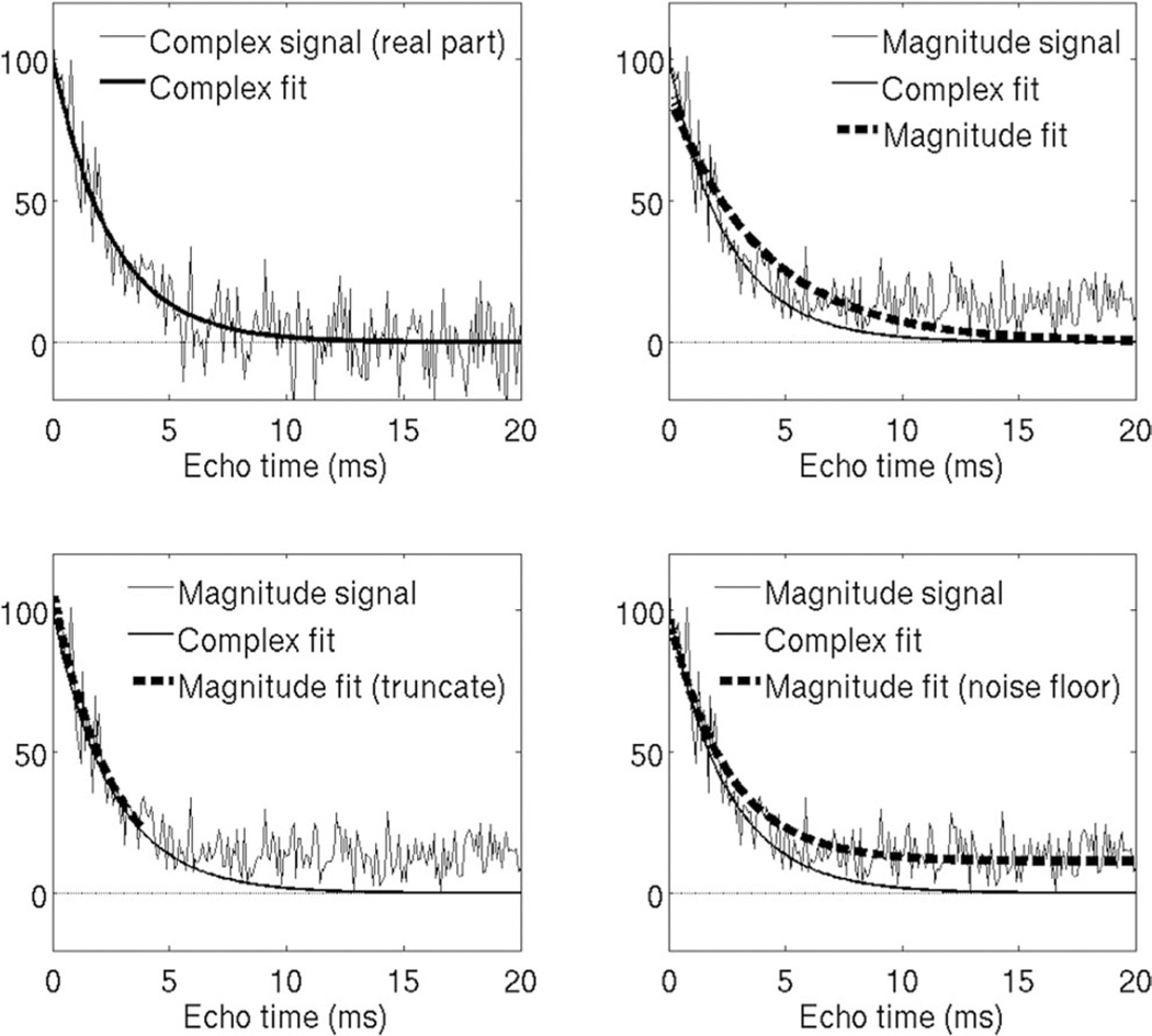
To overcome this limitation of magnitude fitting, several methods have been proposed, most notably baseline fitting, based on introducing an additional parameter C in Eq. [2] to approximately capture the noise floor) (12). The parameter C can be estimated a priori (12) or jointly with ρ_W and R2*. Another common technique for noise floor correction is based on signal truncation (11,27), where one or more echoes at the end of the echo train are discarded to avoid noise floor effects. Figure 1 shows the effect of noise floor on magnitude fitting techniques, including corrections based on noise floor fitting and truncation. Well-known limitations of these methods are their approximated nature (since they do not account for the Rician distribution of noisy magnitude data), and most importantly, the need to estimate the SNR at each voxel, which introduces significant complexity in R2* mapping. In this work, we chose to include analysis of the model including the constant background term C, even though it is not correct (10), because it is very commonly used in recent publications (12,28,29). Similarly, we chose to analyze the truncation technique, even though it does not directly address the Rician distribution of noisy magnitude data (10), because it is also commonly used in recent studies (27,30).

FIG. 1.

Simulation example showing noise floor effects on complex and magnitude fitting R2* estimation techniques, in the presence of rapid signal decay (high R2* = 400 s⁻¹). (Top left) Complex fitting avoids noise bias because the gaussian zero-mean noise is preserved. (Top right) Noisy magnitude signals contain a “noise floor” at low SNR, and magnitude fitting attempts to fit this noise floor, resulting in negative bias in R2* estimation. (Bottom left) Truncation partially corrects this bias by discarding samples below a certain SNR. This typically requires estimation of SNR on a per-pixel basis. (Bottom right) Noise floor fitting techniques attempt to model the noise floor by adding a constant to the signal model. This results in improved fitting of the signal, but does not model the signal behavior accurately, and thus may not correct bias in magnitude fitting.

Fortunately, complex fitting of the signal model in Eq. [1] avoids the complications inherent to magnitude fitting, because the gaussian distribution of the noisy data is preserved (31). With complex fitting, correction algorithms such as baseline fitting or truncation are avoided. In addition, if the field inhomogeneity (f_B) is of interest, this parameter is also provided as part of the complex estimation.

Addressing the Presence of Fat

In the presence of water and fat signal components, the signal acquired at a single voxel can be modeled by the following noise-free signal equation:

$$s_n({\mathrm{\rho }}_{\mathrm{W}},{\mathrm{\rho }}_{\mathrm{F}},{\mathrm{\varphi }}_0,f_{\mathrm{B}},R_2^{*})=({\mathrm{\rho }}_{\mathrm{W}}+{\mathrm{\rho }}_{\mathrm{F}}\sum _{p=1}^P{\alpha }_p{e}^{i2\mathrm{\pi }{f}_{\mathrm{F},p}T{E}_n})e^{i({\mathrm{\varphi }}_0+2\mathrm{\pi }{f}_{\mathrm{B}}T{E}_n)}{e}^{-R_2^{*}T{E}_n}$$ [3]

where ρ_W and ρ_F are the amplitudes of water and fat signals, respectively, with initial phase ϕ₀, R2* = 1/T2*, f_B is the frequency shift due to local magnetic field inhomogeneities, f_F,p are the known frequencies for the multiple spectral peaks of the fat signal relative to the water peak, α_p are the relative amplitudes of the fat signal such that ${\sum }_{\mathrm{p}=1}^{\mathrm{p}}{\alpha }_p=1$ (25). The values of α_p and f_F,p used in this work are those based on measurements made in 121 patients with hepatic steatosis by Hamilton et al. (21). Note that this model assumes a common R2* decay rate for the water and fat signals (“single-R2*” model). This model has been demonstrated to be accurate in previous phantom (32), pre-clinical (33), and clinical studies (34–36). The signal model in Eq. [3] allows for simultaneous water-fat separation (corrected for R2*) and R2* estimation (corrected for the presence of fat).

Similar to the fat-uncorrected case described above (Eq. [2]), fat-corrected R2* estimation can also be performed from magnitude data. In this case, the signal model reduces to:

$$|s_n({\mathrm{\rho }}_{\mathrm{W}},{\mathrm{\rho }}_{\mathrm{F}},R_2^{*})|=|{\mathrm{\rho }}_{\mathrm{W}}+{\mathrm{\rho }}_{\mathrm{F}}\sum _{p=1}^P{\alpha }_p{e}^{i2\mathrm{\pi }{f}_{\mathrm{F},p}T{E}_n}|e^{-R_2^{*}T{E}_n}$$ [4]

where the parameters ϕ₀ and f_B have been eliminated because they only affect the phase of the acquired signal. Note that the fat signal effects (with multiple resonances with different frequencies and relative amplitudes) remain in Eq [4] because they affect the magnitude of the signal. Although noise-floor effects will also affect fat-corrected R2* mapping, correction methods such as baseline fitting or truncation are not commonly used (likely because they introduce additional complexity and noise instability to the estimation problem), and therefore these noise floor correction methods are not considered in this work.

METHODS

Magnitude Versus Complex R2* Relaxometry

Monte-Carlo simulations were performed to assess the bias and standard deviation of R2* estimation using magnitude fitting (without and with noise floor corrections), and complex fitting. A 12-echo acquisition (TE_init = 1.0 ms, ΔTE = 1.0 ms) was simulated, with SNR = 50 at TE = 0 ms and a range of R2* values from 0 to 1200 s⁻¹. A total of 4096 trials were used to measure mean and standard deviation for each reconstruction.

Addressing the Presence of Fat

Monte-Carlo simulations were performed to assess the bias introduced by fat-uncorrected R2* measurements in the presence of fat. Signals at 1.5T were simulated with several 6-TE combinations, using TE_init = 1.0 ms and various echo spacings ΔTE = 1.0, 2.0, 2.3, and 4.6 ms. Simulations were performed at low R2* values (40 s⁻¹) and at very high R2* values (1000 s⁻¹), using a range of fat-fractions from 0 to 100%. A total of 4096 trials were used, with initial SNR = 50 at TE = 0 ms. R2* estimation was performed using fat-uncorrected complex fitting and the bias in R2* was calculated for each echo combination.

Noise Performance of Fat-Corrected Complex and Magnitude R2* Relaxometry

In this section we analyze the noise performance of R2* mapping, as a function of R2* value and TE combination. Further, we study the effect of including fat-correction in R2* mapping. Previously, it has been unknown whether including an additional parameter (fat signal amplitude) in the R2* measurement degrades the SNR performance of R2* mapping due to increased degrees of freedom, i.e., the need to estimate more unknown variables from the same data. To evaluate the noise performance of fat-corrected R2* mapping, we performed theoretical calculations using CRB analysis, as well as Monte-Carlo simulations. The CRB provides a lower bound on the variance of any unbiased estimator, and thus is a useful tool to assess the impact of different acquisition parameters or signal models on the noise performance of the corresponding estimates. Please see Appendix for calculation of the CRB for fat-corrected complex R2* estimation. Monte-Carlo simulations were carried out by simulating signals using the signal model in Eq. [3], adding complex gaussian noise, and performing parameter estimation using NLLS. Calculations were performed for the case with no fat, and with R2* values between 0 and 600 s⁻¹. Simulation parameters were as follows: field strength = 1.5 T, TE_init = 1 ms, ΔTE = 2 ms, and SNR = 50. R2* maps were reconstructed using fat-uncorrected and fat-corrected reconstructions. Bias and standard deviation were computed based on Monte-Carlo simulations, and standard deviation was computed based on CRB analysis.

Optimization of Acquisition Parameters for Fat-Corrected Complex R2* Relaxometry

The choice of acquisition parameters can have a significant impact on the noise performance of R2* mapping. Note that, in contrast to the fat-water separation problem (37), there is no single choice of TE that leads to optimal noise performance for any specific R2* value. The key choice in the design of acquisition parameters is the TE combination (TE_init, ΔTE, number of echoes). However, these parameters are subject to hardware constraints (e.g., limited gradient amplitude and slew rate), and scan time constraints (e.g., breath-hold).

To evaluate the theoretical R2* noise performance for various TE combinations, we performed CRB-based standard deviation for R2* mapping, under the following conditions:

• 6-echo acquisitions as a function of initial TE and TE spacing,

• four different fitting models (fat-uncorrected complex fitting, fat-corrected complex fitting, fat-uncorrected magnitude fitting, fat-corrected magnitude fitting),

• four clinically relevant values of R2* (40, 100, 200, and 1000 s⁻¹), covering a range from normal liver to severe iron overload at 1.5T.

Fat-Corrected R2* Fitting Techniques with Very High R2* Values

For very high R2* values, the choice of complex fitting method becomes very important to maximize the dynamic range of the method by obtaining the best possible noise performance. There are several different techniques available to perform fat-corrected R2* mapping. The original T2*-IDEAL algorithm is based on initial demodulation of the effects of B0 inhomogeneity and R2* decay from the acquired signal, followed by subsequent fat-water separation on the “corrected” signal (25). This method performs well for moderate R2* values but the noise amplification in later echoes introduced by the R2* demodulation results in poor performance for high R2* values. To overcome this limitation, weighted least squares T2*-IDEAL (WLS T2*-IDEAL) was introduced by Vasanawala et al (31). In this work, the fat-water separation was performed weighting less those echoes with lower SNR, thus preventing excessive noise propagation from these echoes. An alternative is to perform a descent-based NLLS fitting where all unknown parameters (water, fat, R2*, and B0 field) are estimated jointly (26). NLLS also has the advantage that it can be performed using magnitude data (38).

Monte-Carlo simulations were performed to test the bias and noise performance of these fat-corrected reconstruction algorithms (T2*-IDEAL, WLS-T2*-IDEAL, magnitude NLLS, and complex NLLS) over a range of R2* values (0–1200 s⁻¹), and using two different 6-echo combinations: “standard 1.5T” TEs (TE_init = 1 ms and ΔTE = 2 ms), and short TEs (TE_init = 0.4 ms and ΔTE = 0.8 ms). Further, these algorithms were used to reconstruct a 3T liver dataset on a patient with severe iron overload, acquired using a multiecho 3D SPGR acquisition with TE_init = 1 ms, ΔTE = 1 ms.

In Vivo Validation

To evaluate the need for fat-corrected R2* mapping, we assessed the robustness of R2* measurements using different fitting models for liver imaging, in subjects with varying levels of liver fat. Robustness was assessed by reconstructing data from each subject using different TE combinations, and comparing the resulting R2* measurements. Ideally, R2* estimation should be independent (i.e., robust) of the choice of TE combination. However, R2* reconstructions that do not accurately model the signal may result in severe variability in the measured R2* as a function of the choice of TEs (both the number of echoes and the specific TE).

This institutional review board approved, HIPAA compliant study included 28 patients that underwent abdominal MR imaging for a variety of reasons not limited to fatty liver disease (cancer staging, lesion characterization, etc.) between 03/2008 and 10/2009. The patient population included in this study has been evaluated in prior studies with regard to the hepatic proton density fat-fraction (35,39); however, the robustness of R2* mapping has not been previously investigated.

Liver datasets from the 28 subjects were retrospectively reconstructed. Imaging was performed at 1.5T (Signa HDxt; GE Healthcare, Waukesha, WI) using an eight-channel phased-array torso coil. A multiecho 3D SPGR acquisition was performed on the liver, using fly-back readout gradients. Imaging parameters included are as follows: 6 echoes/TR, TR = 13.7 ms, TE₁ = 1.3 ms, ΔTE = 2.0 ms, bandwidth = ± 125 kHz, FOV = 35 × 35 cm, flip angle = 5° to minimize T1 related bias, matrix = 256 × 128, 24 cm coverage in the S-I direction, parallel imaging acceleration with acceleration = 2.2, and slice thickness = 10 mm.

Additionally, single-voxel spectroscopy was acquired in each subject for fat-quantification. Spectroscopy was performed as described in (39) using a STEAM sequence to minimize J-coupling effects (40), and used five TE between 10 and 50 ms to correct for T2 decay in the quantification of liver fat.

To test the robustness of different reconstructions, datasets were reconstructed using different echo combinations: the first 3, 4, 5, and all 6 echoes. Magnitude and complex fitting was used in each case, including fat-uncorrected, fat-corrected (single-peak fat modeling), and fat-corrected (multipeak fat modeling), for a total of six R2* reconstructions per dataset and echo combination. R2* measurements were obtained by a radiologist with 9 years experience in liver imaging. These measurements were co-localized with the spectroscopy voxel in each subject. Spectroscopy provided a fat-fraction measurement for each subject (39).

For each subject and each reconstruction model, the R2* values estimated using different numbers of echoes were compared. Note that, in the absence of a reference standard for R2*, a desirable quality for a quantitative imaging biomarker such as R2* is robustness: the ability to produce the same quantitative measurements from different imaging acquisition protocols (e.g., different TE combinations). As a measure of robustness for each reconstruction model, the R2* standard deviation over N_echoes = 4, 5, 6 was recorded for each subject. For this analysis, N_echoes = 3 was excluded due to instabilities in fat-corrected reconstructions from 3 echoes. Ideally, R2* standard deviation should be zero (i.e., all TE combinations result in the same R2* measurement) regardless of the fat-fraction and acquisition parameters. The relationship between the observed standard deviation and the fat-fraction was determined using a linear regression analysis.

RESULTS

Magnitude Versus Complex R2* Relaxometry

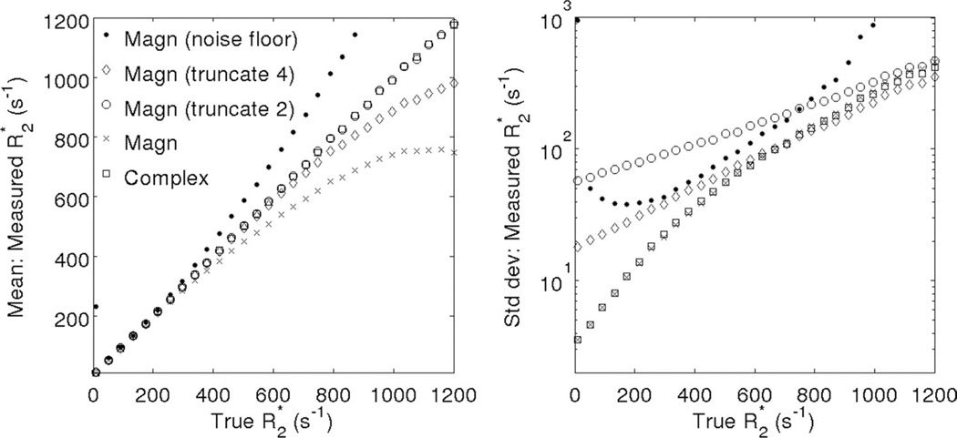
Figure 2 shows simulation results (bias and standard deviation) for magnitude and complex R2* fitting methods. Magnitude fitting R2* mapping results in protocol-dependent errors in R2* quantification. Baseline correction by jointly fitting for the baseline C results in large bias and noise amplification, particularly at low R2* values (where the decaying signal itself looks similar to a constant), and at very high R2* values (where the introduction of an additional parameter results in increased noise sensitivity) (13). Truncation results in a more straightforward compromise between bias and standard deviation. More truncation leads to reduced bias, but at the cost of increased standard deviation. Sophisticated techniques have been developed for automatic selection of truncation levels (27). These methods essentially involve estimation of the noise floor at each voxel and have been shown to perform better than methods based on a global noise floor. However, these methods introduce significant complexity to provide a good tradeoff between noise and bias, and may result in some SNR loss due to discarding echoes with low (but nonzero) SNR.

FIG. 2.

Compared with magnitude fitting techniques, complex fitting results in R2* measurements with very low bias over a large range of R2* values. Plots show Monte-Carlo simulation results from a 12-echo acquisition (TE_init = 1.0 ms, ΔTE = 1.0 ms), including (left) mean and (right) standard deviation of R2* estimates obtained using magnitude fitting (including noise floor fitting, two levels of truncation (“truncate 4”: keep the first four echoes only and “truncate 2”: keep the first two echoes only) as well as fitting all the echoes (with no noise correction), and complex fitting (no noise correction needed). Standard deviation was determined from a Monte-Carlo simulation using 4096 trials with SNR = 50 at TE = 0.

Noise floor related errors can be ameliorated in the context of magnitude fitting using several approximated correction techniques, or completely avoided using complex fitting. Complex fitting is able to maintain low bias and good SNR over a wide range of R2* values and TE combinations.

Addressing the Presence of Fat

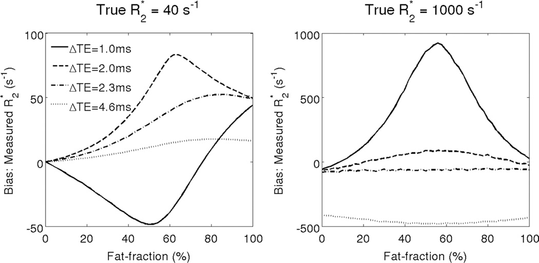
Figure 3 shows simulation results for the R2* bias obtained with fat-uncorrected R2* measurements in the presence of varying levels of fat and no noise. The bias worsens with increasing amount of fat and is highly dependent on the choice of TE used for the R2* fitting. Note that the bias does not return to zero when there is 100% fat. This occurs because the spectral complexity of fat leads to a complex interference pattern between the peaks of fat, causing incorrect estimation of R2*. Indeed, it has recently been demonstrated that improved accuracy in R2* mapping is obtained by performing fat-corrected reconstruction using a multi-peak fat signal model (41). Additionally, note that at high R2* values, the effects of fat and noise floor will contribute to additional bias when magnitude-based reconstruction methods are used. This protocol-dependent bias in fat-uncorrected R2* mapping results in poor robustness in R2* mapping the presence of fat.

FIG. 3.

If fat is not considered in the signal model, very large bias can occur when performing R2* estimation. Fat-uncorrected R2* mapping results in severe protocol-dependent bias when fat is present in tissue. The plots show simulation results for the bias obtained at 1.5T with complex fitting using several 6-TE combinations, with TE_init = 1.0 ms and various echo spacings ΔTE = 1.0, 2.0, 2.3, and 4.6 ms. Large bias can occur both at low R2* values (40 s⁻¹) and at high R2* values (1000 s⁻¹). Note that fat-uncorrected R2* estimates show poor robustness to varying TE combinations in the presence of fat. The bias does not return to zero at 100% fat because the spectral complexity of fat leads to complex interference patterns between the peaks of fat that lead to incorrect estimates of R2*.

Noise Performance of Fat-Corrected Complex and Magnitude R2* Relaxometry

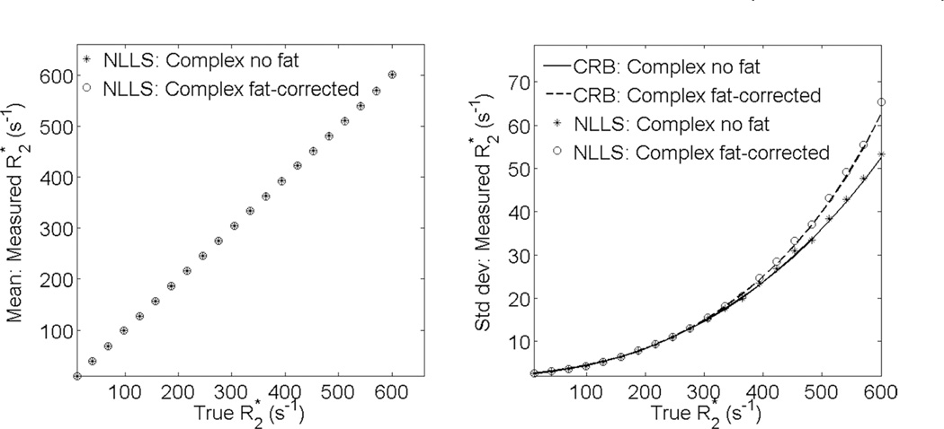
Figure 4 shows the mean and standard deviation for fat-corrected complex R2* fitting vs fat-uncorrected complex R2* fitting. Note the good agreement in the standard deviation between theoretical (CRB) calculations, and Monte-Carlo simulations. For typical TE combinations, fat-corrected R2* estimation demonstrates no bias over a broad range of R2* values, and imposes virtually no SNR penalty for R2* < 300 s⁻¹, and a moderate penalty for R2* < 600 s⁻¹, compared with a signal model not accounting for fat. At higher values of R2* > 600 s⁻¹, shorter TE (or higher SNR) are required to avoid bias in fat-corrected reconstructions (as described below).

FIG. 4.

Fat-corrected R2* mapping results in no bias and no SNR penalty over a wide range of R2* values. The plots contain simulation results showing (left) mean and (right) standard deviation for complex-fitting using NLLS fat-uncorrected and fat-corrected R2* estimates in the absence of fat. Simulation parameters were as follows: 6 echoes, TE_init = 1 ms, ΔTE = 2 ms, and initial SNR = 50. In the absence of fat, both techniques provide the same mean. Both techniques provide standard deviation matching theoretical predictions (CRB). Fat-corrected R2* has essentially no SNR penalty up to R2* = 300 s⁻¹, and only a modest penalty up to R2* = 600 s⁻¹. For higher R2* values, a moderate bias is incurred with this choice of TE, and shorter echoes are required to obtain accurate fat-corrected R2* measurements.

Optimization of Acquisition Parameters for Fat-Corrected Complex R2* Relaxometry

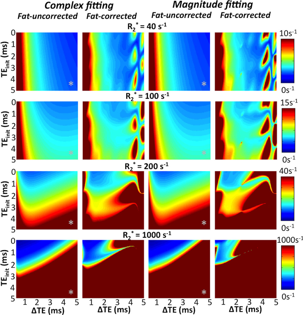
As shown in Figures 5 and 6, fat-corrected R2* mapping results in no or moderate SNR penalty (relative to fat-uncorrected R2*), for a wide range of TE combinations and R2* values. Interestingly, magnitude fitting performs very similarly to complex fitting for moderate R2* values. In contrast to magnitude-based fat-water separation, fat-corrected magnitude R2* fitting does not break down for certain TE combinations, e.g., near (TE_init = 1.3 ms, ΔTE = 2.2 ms) (42,43). Note that this noise performance analysis does not consider noise floor bias. As discussed above, magnitude fitting will only perform well at moderate R2* values.

FIG. 5.

Theoretical noise performance (standard deviation) of R2* estimation at 1.5T for 6-echoes using various TE combinations [as a function of initial TE_min and echo spacing (ΔTE)]. Plots include four different reconstruction techniques (fat-uncorrected complex, fat-corrected complex, fat-uncorrected magnitude, fat-corrected magnitude), and four different true R2* values (40, 100, 200, and 1000 s⁻¹). The plots depict the strong dependence of noise performance on the choice of TEs, and the lack of a globally optimal (for all R2* values) TE combination. Note the lack of noise penalty of fat-corrected reconstructions over a wide range of TE combinations. Magnitude reconstructions introduce only a slight noise penalty relative to complex reconstructions, although this analysis does not include noise-related bias. Finally, “inphase” acquisitions (marked with “*”) can be used instead of fat-corrected reconstructions to approximately correct for the presence of fat, but these result in severe noise amplification at high R2* values.

FIG. 6.

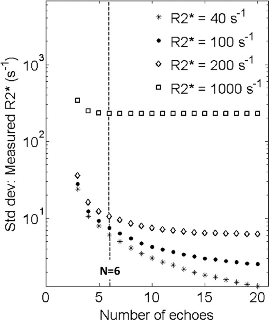
The optimum number of echoes for fat-corrected R2* mapping is heavily dependent on the underlying R2* value. Plots shows the theoretical noise performance (standard deviation) of fat-corrected R2* mapping as a function of number of TEs, for fixed initial TE (1 ms) and echo spacing (1 ms). Except for low values of R2* (e.g., 40 s⁻¹), there is little benefit to increasing the echo train length beyond 6. Even with 6 echoes, the noise performance of R2* estimation when R2* = 40 s⁻¹, is very good because the signal levels are high compared with tissue with high R2*.

As shown in Figure 5, short echoes (e.g., TE_init < 1 ms, ΔTE = 1 ms) are essential for R2* mapping in the presence of very high R2* values, as they result in much improved noise performance. As expected, at high R2* values, short TEs perform better with every model. Note that acquisition of “in-phase” echoes (TE_init = 4.6 ms, ΔTE = 4.6 ms; marked with “*” on the maps in Fig. 5) used to correct for fat (to first approximation) leads to very poor noise performance for high R2* values. Instead, it is preferable to acquire closely spaced echoes and perform fat-corrected R2* mapping through fat-corrected R2* estimation. Short TEs typically also result in acceptable (although not optimal) R2* noise performance for low to moderate R2* values.

Finally, the effect of the number of echoes acquired was also investigated. Figure 6 shows the theoretical noise performance of complex fat-corrected R2* mapping for fixed TE_init = 1 ms, ΔTE = 1 ms, with varying numbers of echoes. Note that acquiring additional echoes (beyond 6) results in improved (reduced) standard deviation in the R2* estimate for low R2* values, but not for high R2* = 1000 s⁻¹, where most of the signal has fully decayed by TE = 3–4 ms.

The optimal choice of TE combination and number of echoes depends on the specific application and range of possible R2* values. A reasonable approach may be to optimize the acquisition for the high range of expected R2* values, where, to obtain accurate R2* measurements, it is critical to acquire several echoes before the signal disappears.

Fat-Corrected R2* Fitting Techniques with Very High R2* Values

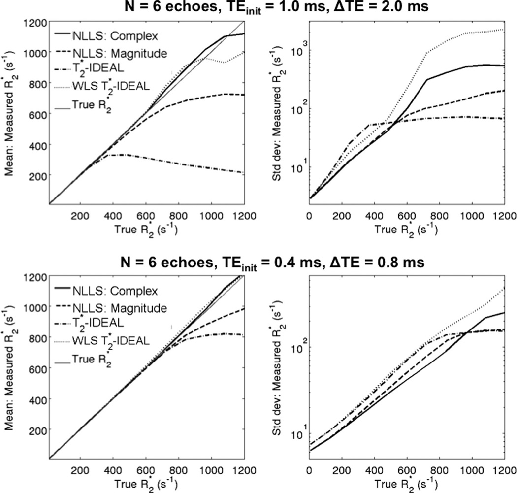
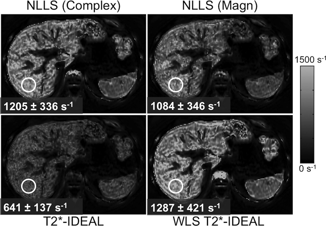
Figure 7 shows simulation results (mean and standard deviation) for fat-corrected R2* mapping using the four techniques described above (T2*-IDEAL, WLS T2*-IDEAL, complex NLLS, and magnitude NLLS). R2* mapping was performed using two different 6-echo TE combinations (one with “standard” TEs and one with short TEs), and for a range of R2* values between 40 and 1200 s⁻¹. As expected, all methods perform well for moderate R2* values. T2*-IDEAL “breaks down” for R2* > 400 s⁻¹ (long TEs) and for R2* > 800 s⁻¹ (short TEs), similarly to magnitude NLLS. WLS T2*-IDEAL is largely able to correct the bias in T2*-IDEAL. However, both have relatively poor noise performance at high R2* values. Complex NLLS achieves low bias with relatively good noise performance over a broad range of R2* values and for both choices of TE combination. Figure 8 shows in vivo 3T R2* mapping results from a subject with liver iron overload. The relative bias between the different reconstruction techniques is in good qualitative agreement with simulation results.

FIG. 7.

Simulation results using multiple fat-corrected R2* reconstruction algorithms, for two different TE combinations. All methods perform well at low to moderate R2* values. At high R2* values, T2*-IDEAL and magnitude NLLS result in significant bias. Both WLS T2*-IDEAL and complex NLLS avoid bias for a wide range of R2* values. However, for extreme R2* values (~1000 s⁻¹), short TEs (bottom) are needed to avoid bias with either reconstruction. Note the superior noise performance (reduced standard deviation) of complex NLLS relative to WLS T2*-IDEAL. The low standard deviation of conventional T2*-IDEAL at high R2* values is overshadowed by very high bias.

FIG. 8.

Complex fitting with nonlinear LS or WLS-IDEAL provide a broad dynamic range for R2* measurement. Alternative techniques such as magnitude NLLS fitting or (unweighted) T2*-IDEAL result in significant bias at high R2* values. Images show liver R2* maps (6 echoes, TE_init = 1 ms, ΔTE = 1 ms) at 3.0T from a patient with severe iron overload.

In Vivo Validation

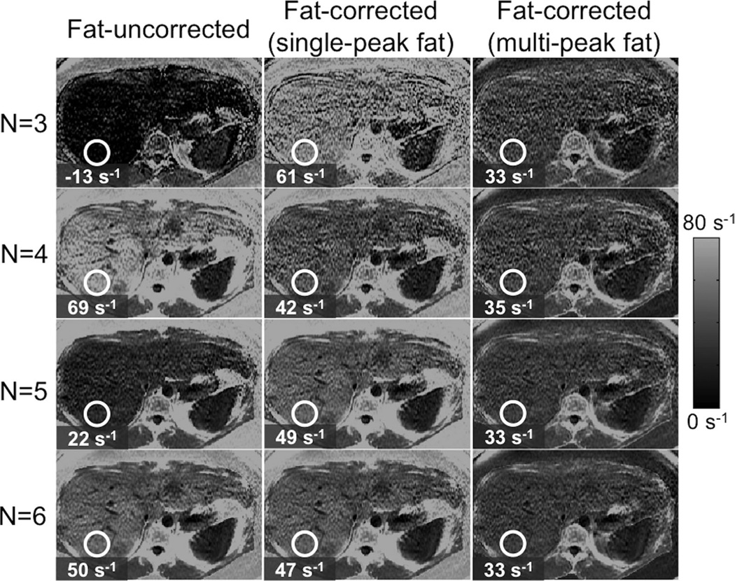
Figure 9 shows example R2* reconstructions in a subject with high liver fat (fat-fraction = 34%), from an acquisition with six echoes, TE₁ = 1.3 ms, ΔTE = 2.0 ms. Three different reconstructions were performed: fat-uncorrected, fat-corrected (single-peak fat model), and fat-corrected (multipeak fat model). Each reconstruction was performed with different TE combinations: using the first 3, 4 5, and all 6 echoes, respectively. Fat correction including multipeak fat is necessary for robust R2* mapping.

FIG. 9.

Fat-correction using multipeak fat modeling is necessary for robust R2* mapping in the presence of fat. Images show liver R2* maps on a subject with high liver fat (fat-fraction = 34%), using three different techniques (fat-uncorrected, fat-corrected with single-peak fat and fat-corrected with multipeak fat) and four different TE combinations (3, 4, 5, and 6 echoes). Note the decrease in R2* mapping noise for increasing number of echoes. Fat-uncorrected and single-peak R2* measurements show variability with echo combination, whereas fat-corrected R2* estimates demonstrates excellent robustness to echo combination. Note also the very high apparent R2* in subcutaneous tissue when not accounting for multipeak fat effects.

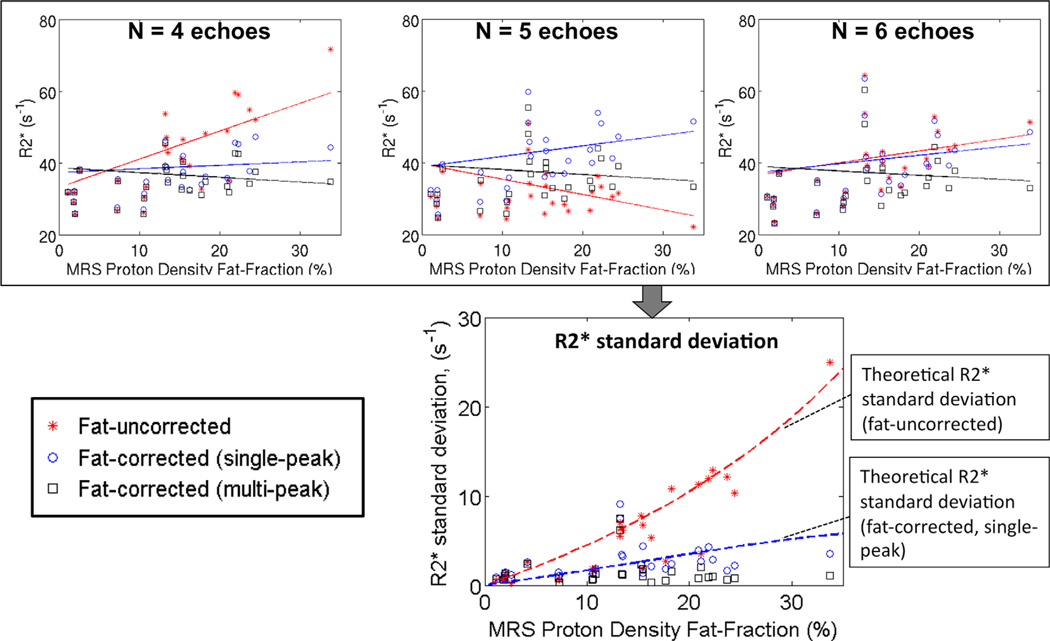
Figure 10 shows robustness results for all 28 subjects, and numbers of echoes 4, 5, and 6. At low fat-fractions, all methods perform similarly. At high fat-fractions, fat-uncorrected R2* measurements result in poor robustness (high variability in co-localized R2* measurements obtained from different TE combinations). Robustness is improved with single-peak fat-corrected modeling, although some residual variations remain at high fat-fractions. Multipeak fat modeling results in the best robustness, particularly at high fat-fractions.

FIG. 10.

Fat-correction using multipeak fat modeling is necessary for robust R2* mapping in the presence of fat. (Top) R2* measurements as a function of PDFF obtained using three different techniques (fat-uncorrected, fat-corrected with single-peak fat and fat-corrected with multipeak fat), from three different TE combinations (4, 5, and 6 echoes). Note that fat-uncorrected R2* reconstructions can show an apparently strong relationship between PDFF and R2* for certain TE combinations. This strong relationship is not present in fat-corrected R2* reconstructions. (Bottom) Plot shows R2* variability (standard deviation) for each reconstruction, as a function of PDFF. Fat-uncorrected and fat-corrected (single-peak) reconstructions result in R2* variability increasing with PDFF, as predicted by theory (dashed lines). Fat-corrected (multipeak) R2* mapping theoretically should result in no variability in the absence of noise, and in practice results in low variability (good robustness) over the entire range of PDFF. [Color figure can be viewed in the online issue, which is available at wileyonlinelibrary.com.]

Linear regression analysis revealed a statistically significant relationship between the standard deviation of fat-uncorrected R2* (as a function of echo combination) and the fat-fraction (r² = 0.86; P < 0.001). Fat-corrected R2* using either single-peak (r² = 0.32; P = 0.09) or multipeak (r² = 0.00; P = 0.99) fat did not show a statistically significant relationship with fat-fraction, although single-peak fat-corrected R2* mapping showed an increasing trend with fat-fraction.

DISCUSSION

To establish R2* (=1/T2*) as a quantitative biomarker, it is important to obtain R2* measurements with low bias and low noise. Bias due to noise floor effects can be significant in magnitude-based reconstructions, particularly at high R2* values. The presence of fat, if uncorrected, can introduce severe protocol-dependent bias both at low and high R2* values. Fat-corrected R2* mapping including modeling of the fat signal spectrum is needed to avoid this bias. Noise performance in R2* measurement is strongly dependent on the choice of TEs and on the true R2* decay rate. In this work, we have shown that complex-fitting fat-corrected R2* reconstructions provide R2* quantification with low bias and low noise over a wide range of TE combinations and R2* values.

Additionally, we have provided a framework to optimize the method and provided some optimal parameters for typical situations. The optimal acquisition parameters (echo combination) depend on the underlying R2*. For high R2*, short TEs are essential to minimize bias and standard deviation. For instance, acquisition schemes that impose a relatively long initial TE, e.g., due to the use of self-navigation (44) are adequate for mapping moderate R2* values, but are limited in the presence of high R2* as is the case in patients with liver iron overload. The need for short TEs has been observed empirically in previous studies (12); however, in this work, we have developed an analytical framework for choosing TE combinations to cover the desired range of R2* values.

For reconstruction of R2* maps, complex fitting avoids bias and provides low standard deviation over a wide range of acquisition parameters and R2* values. Complex fitting has the advantage of avoiding noise floor effects for R2* mapping, and providing generally superior noise performance. Additionally, fat-correction can be performed from a wide choice of TE combinations, providing improved R2* mapping robustness with little or no noise penalty (typically as long as more than 3 echoes are acquired).

Magnitude-based fat-corrected methods (38) also provide R2* measurements free of the effects of fat for a wide range of acquisition parameters. Magnitude fitting methods work well for moderate R2* values, but result in bias at high R2* values (e.g., in the presence of severe iron overload), or at low SNR, due to noise floor effects. It may be possible to reduce this bias using baseline fitting or signal truncation approaches in combination with magnitude-based fat-corrected R2* mapping. However, complex-based fat-corrected methods generally have superior noise performance and are free from noise floor effects.

One limitation of complex-based methods is somewhat increased sophistication of the reconstruction algorithms (e.g., due to the need to account for phase offsets due to B0 inhomogeneities), and the need to modify image reconstruction algorithms to provide complex images. However, it should be noted that advanced magnitude-based reconstruction algorithms that attempt to correct for noise floor effects through truncation methods or baseline fitting also have considerable complexity.

Another limitation of complex methods is the need to estimate R2* voxel-by-voxel. The R2* estimates can then be combined over an ROI. However, due to the presence of B0 inhomogeneities it is problematic to average the signals first and perform R2* estimation only on the averaged signal (which is potentially computationally more efficient and is often done for magnitude-based parametric estimation). Performing fitting directly on the averaged ROI signal will generally affect the bias/noise tradeoff for both complex- and magnitude-fitting techniques. A detailed analysis of this approach is beyond the scope of this work.

In this work, we have shown that complex NLLS fitting has superior performance (in terms of bias and standard deviation), compared with previous techniques that do not directly perform NLLS. Complex NLLS fitting results in the maximum-likelihood estimator in the presence of gaussian noise. Maximum-likelihood estimators are known to be efficient (unbiased and with noise performance matching the CRB) at high SNR. Complex NLLS performs well over a broad range of R2* values and acquisition parameters. However, in this work, we have observed bias in complex fitting, even when using the correct signal model. This bias occurs in cases of low SNR or extreme R2* values unless short enough TEs are employed, and may be significant for applications such as measuring liver iron concentration in patients with severe iron overload (R2* > 1000) (1).

The fat-corrected R2* models used in this work use a “single-R2*” assumption, i.e., they assign a common R2* decay rate to both water and fat components. Potentially, a more sophisticated model using “dual-R2*” (with different R2* values for water and fat) may be potentially more accurate. However, dual-R2* models introduce severe noise amplification, instabilities, and sensitivity to image artifacts, and additionally perform poorly at low fat-fractions. Dual-R2* modeling may be made feasible by different data acquisition schemes (more echoes and higher SNR), or improved reconstruction schemes (imposing prior constraints on the difference between the R2* decay rates of fat and water). However, currently single-R2* reconstruction is more practically viable and has been shown to be robust in this work. Additionally, in previous works single-R2* models were shown to be accurate in fat-water-iron phantoms with realistic fat particle size (32), iron-overloaded mice (33), and in subjects without liver iron overload (35,39).

The in vivo acquisitions used in this work used a low flip angle to minimize T1 bias in fat quantification. We do not expect T1 effects to directly introduce bias on R2* mapping. However, T1 contrast mechanisms may affect the SNR of the acquired images, which in turn may influence the noise floor bias in the measured R2* (particularly for magnitude fitting techniques), leading to an apparent dependence of R2* on T1.

Another confounding factor for R2* mapping, not considered in this work, is the presence of background field variations (e.g., due to magnet imperfections, or susceptibility effects near tissue/air interfaces). In regions of severe background field variation, additional intravoxel dephasing can occur, leading to rapid signal decay and increased apparent R2*. This is particularly problematic when acquiring images with low spatial resolution or thick slices, and it can lead to poor robustness in R2* mapping, as the apparent R2* will be dependent on acquisition parameters (e.g., spatial resolution). Note that background field variations introduce signal dephasing that accelerates the decay of the signal magnitude, therefore affecting both magnitude and complex fitting techniques. Several methods have been proposed to correct for the effect of background field variations in R2*. Specifically, complex fitting has the added advantage of simultaneous estimation of the field inhomogeneity map, which may then be used to model and correct for background field variations (45). However, background field variation effects can be minimized by using high-resolution (thin slices), or performing R2* quantification in regions away from susceptibility artifacts. These results suggest that R2* mapping corrected for relevant confounding factors may provide robust and accurate measurements of liver iron. However, validation of these properties is beyond the scope of this work.

In conclusion, this work has shown that fat-corrected complex-fitting R2* mapping can provide measurements with low bias and low noise over a wide range of R2* values and TE combinations. Additionally, this work has provided a framework for optimally choosing the TE combination for a given expected range of R2* values.

APPENDIX

Calculation of Cramer-Rao Bounds

The CRB provides a lower bound on the variance of any unbiased estimator. For multi-parametric models, the CRB is a matrix providing a lower bound on the covariance matrix of the estimates, and the diagonal elements of the CRB matrix give the CRB for each of the parameters involved.

Consider a set of unknown parameters x = (x₁, x₂, …, x_M) to be estimated from a set of noisy measurements y = (y₁, y₂, …, y_N). In our case, x consists of the unknown parameters at a single voxel (water and fat amplitudes, R2*, B0 offset) and y consists of the measured signals for increasing TEs at that same voxel. The CRB matrix for estimation of x from y is defined as:

$$\mathrm{C}\mathrm{R}\mathrm{B}=F^{-1}$$

where F is the Fisher Information Matrix (FIM). Each element of the FIM is defined as:

$$F_{j,k}=-E\left\{\frac{\partial L(x;y)}{\partial x_j}\frac{\partial L(x;y)}{\partial x_k}\right\}$$

where E denotes expectation value (over the probability distribution of noisy measurements y) and L(x) is the log-likelihood function of the parameters x given the measurements y.

Complex Fitting CRB

For complex-fitting techniques, derivation of the CRB is particularly simple, due to the gaussian distribution of the noisy MR data. In this case, the FIM reduces to (46):

$$F_{j,k}=-\frac{1}{{\mathrm{\sigma }}^2}\sum _{n=1}^N\frac{\partial s_n}{\partial x_j}\frac{\partial s_n}{\partial x_k}$$

where s_n is the noiseless complex signal described in Eq. [3].

Magnitude Fitting CRB

For magnitude-fitting techniques, the noisy data follows a Rician distribution. In this case, the FIM is defined as (47):

$$F_{j,k}=-\frac{1}{{\mathrm{\sigma }}^2}\sum _{n=1}^N\frac{\partial s_n}{\partial x_j}\frac{\partial s_n}{\partial x_k}\left[E\right\{\frac{y_n^2}{{\mathrm{\sigma }}^2}\frac{I_1^2(y_n{s}_n/{\mathrm{\sigma }}^2)}{I_0^2(y_n{s}_n/{\mathrm{\sigma }}^2)}\}-\frac{s_n^2}{\mathrm{\sigma }}]$$

where y_n is the noisy data given the noiseless magnitude signal s_n (defined in Eq. [4]), and I₀ and I₁ are modified Bessel functions of the first kind, of zeroth and first order, respectively.

REFERENCES

- 1.Wood JC, Enriquez C, Ghugre N, Tyzka JM, Carson S, Nelson MD, Coates TD. MRI R2 and R2* mapping accurately estimates hepatic iron concentration in transfusion-dependent thalassemia and sickle cell disease patients. Blood. 2005;106:1460–1465. doi: 10.1182/blood-2004-10-3982. [DOI] [PMC free article] [PubMed] [Google Scholar]
- 2.Schwenzer NF, Machann J, Haap MM, et al. T2* relaxometry in liver, pancreas, and spleen in a healthy cohort of one hundred twenty-nine subjects-correlation with age, gender, and serum ferritin. Invest Radiol. 2008;43:854–860. doi: 10.1097/RLI.0b013e3181862413. [DOI] [PubMed] [Google Scholar]
- 3.Anderson LJ, Holden S, Davis B, et al. Cardiovascular T2-star (T2*) magnetic resonance for the early diagnosis of myocardial iron over-load. Eur Heart J. 2001;22:2171–2179. doi: 10.1053/euhj.2001.2822. [DOI] [PubMed] [Google Scholar]
- 4.Ordidge RJ, Gorell JM, Deniau JC, Knight RA, Helpern JA. Assessment of relative brain iron concentrations using T2-weighted and T2*-weighted MRI at 3 Tesla. Magn Reson Med. 1994;32:335–341. doi: 10.1002/mrm.1910320309. [DOI] [PubMed] [Google Scholar]
- 5.Ogawa S, Menon RS, Tank DW, Kim SG, Merkle H, Ellermann JM, Ugurbil K. Functional brain mapping by blood oxygenation level-dependent contrast magnetic resonance imaging. A comparison of signal characteristics with a biophysical model. Biophys J. 1993;64:803–812. doi: 10.1016/S0006-3495(93)81441-3. [DOI] [PMC free article] [PubMed] [Google Scholar]
- 6.Sadowski EA, Djamali A, Wentland AL, Muehrer R, Becker BN, Grist TM, Fain SB. Blood oxygen level-dependent and perfusion magnetic resonance imaging: detecting differences in oxygen bioavailability and blood flow in transplanted kidneys. Magn Reson Imaging. 2010;28:56–64. doi: 10.1016/j.mri.2009.05.044. [DOI] [PMC free article] [PubMed] [Google Scholar]
- 7.Kuhlpeter R, Dahnke H, Matuszewski L, Persigehl T, von Wallbrunn A, Allkemper T, Heindel WL, Schaeffter T, Bremer C. R2 and R2* mapping for sensing cell-bound superparamagnetic nanoparticles: in vitro and murine in vivo testing. Radiology. 2007;245:449–457. doi: 10.1148/radiol.2451061345. [DOI] [PubMed] [Google Scholar]
- 8.McVeigh ER, Henkelman RM, Bronskill MJ. Noise and filtration in magnetic resonance imaging. Med Phys. 1985;12:586–591. doi: 10.1118/1.595679. [DOI] [PMC free article] [PubMed] [Google Scholar]
- 9.Henkelman RM. Measurement of signal intensities in the presence of noise in MR images. Med Phys. 1985;12:232–233. doi: 10.1118/1.595711. [DOI] [PubMed] [Google Scholar]
- 10.Gudbjartsson H, Patz S. The Rician distribution of noisy MRI data. Magn Reson Med. 1995;34:910–914. doi: 10.1002/mrm.1910340618. [DOI] [PMC free article] [PubMed] [Google Scholar]
- 11.He T, Gatehouse PD, Smith GC, Mohiaddin RH, Pennell DJ, Firmin DN. Myocardial T2* measurements in iron-overloaded thalassemia: an in vivo study to investigate optimal methods of quantification. Magn Reson Med. 2008;60:1082–1089. doi: 10.1002/mrm.21744. [DOI] [PMC free article] [PubMed] [Google Scholar]
- 12.Ghugre NR, Enriquez CM, Coates TD, Nelson MD, Jr, Wood JC. Improved R2* measurements in myocardial iron overload. J Magn Reson Imaging. 2006;23:9–16. doi: 10.1002/jmri.20467. [DOI] [PMC free article] [PubMed] [Google Scholar]
- 13.Carneiro AA, Baffa O, Fernandes JP, Zago MA. Theoretical evaluation of the susceptometric measurement of iron in human liver by four different susceptometers. Physiol Meas. 2002;23:683–693. doi: 10.1088/0967-3334/23/4/308. [DOI] [PubMed] [Google Scholar]
- 14.Wehrli FW, Ma J, Hopkins JA, Song HK. Measurement of R′2 in the presence of multiple spectral components using reference spectrum deconvolution. J Magn Reson. 1998;131:61–68. doi: 10.1006/jmre.1997.1327. [DOI] [PubMed] [Google Scholar]
- 15.Szczepaniak LS, Nurenberg P, Leonard D, Browning JD, Reingold JS, Grundy S, Hobbs HH, Dobbins RL. Magnetic resonance spectroscopy to measure hepatic triglyceride content: prevalence of hepatic steatosis in the general population. Am J Physiol Endocrinol Metab. 2005;288:E462–E468. doi: 10.1152/ajpendo.00064.2004. [DOI] [PubMed] [Google Scholar]
- 16.Hu HH, Kim HW, Nayak KS, Goran MI. Comparison of fat-water MRI and single-voxel MRS in the assessment of hepatic and pancreatic fat fractions in humans. Obesity (Silver Spring) 2010;18:841–847. doi: 10.1038/oby.2009.352. [DOI] [PMC free article] [PubMed] [Google Scholar]
- 17.Goodpaster BH, Stenger VA, Boada F, McKolanis T, Davis D, Ross R, Kelley DE. Skeletal muscle lipid concentration quantified by magnetic resonance imaging. Am J Clin Nutr. 2004;79:748–754. doi: 10.1093/ajcn/79.5.748. [DOI] [PubMed] [Google Scholar]
- 18.Kellman P, Hernando D, Shah S, Zuehlsdorff S, Jerecic R, Mancini C, Liang ZP, Arai AE. Multiecho dixon fat and water separation method for detecting fibrofatty infiltration in the myocardium. Magn Reson Med. 2009;61:215–221. doi: 10.1002/mrm.21657. [DOI] [PMC free article] [PubMed] [Google Scholar]
- 19.Wehrli FW, Ford JC, Haddad JG. Osteoporosis: clinical assessment with quantitative MR imaging in diagnosis. Radiology. 1995;196:631–641. doi: 10.1148/radiology.196.3.7644622. [DOI] [PubMed] [Google Scholar]
- 20.Dahnke H, Schaeffter T. Limits of detection of SPIO at 3.0 T using T2 relaxometry. Magn Reson Med. 2005;53:1202–1206. doi: 10.1002/mrm.20435. [DOI] [PubMed] [Google Scholar]
- 21.Hamilton G, Yokoo T, Bydder M, Cruite I, Schroeder ME, Sirlin CB, Middleton MS. In vivo characterization of the liver fat (1)H MR spectrum. NMR Biomed. 2011;24:784–790. doi: 10.1002/nbm.1622. [DOI] [PMC free article] [PubMed] [Google Scholar]
- 22.Bydder GM, Steiner RE, Blumgart LH, Khenia S, Young IR. MR imaging of the liver using short TI inversion recovery sequences. J Comput Assist Tomogr. 1985;9:1084–1089. doi: 10.1097/00004728-198511000-00015. [DOI] [PubMed] [Google Scholar]
- 23.Haase A, Frahm J, Hanicke W, Matthaei D. 1H NMR chemical shift selective (CHESS) imaging. Phys Med Biol. 1985;30:341–344. doi: 10.1088/0031-9155/30/4/008. [DOI] [PubMed] [Google Scholar]
- 24.Meyer CH, Pauly JM, Macovski A, Nishimura DG. Simultaneous spatial and spectral selective excitation. Magn Reson Med. 1990;15:287–304. doi: 10.1002/mrm.1910150211. [DOI] [PubMed] [Google Scholar]
- 25.Yu H, Shimakawa A, McKenzie CA, Brodsky E, Brittain JH, Reeder SB. Multiecho water-fat separation and simultaneous R2* estimation with multifrequency fat spectrum modeling. Magn Reson Med. 2008;60:1122–1134. doi: 10.1002/mrm.21737. [DOI] [PMC free article] [PubMed] [Google Scholar]
- 26.Hernando D, Liang ZP, Kellman P. Chemical shift-based water/fat separation: a comparison of signal models. Magn Reson Med. 2010;64:811–822. doi: 10.1002/mrm.22455. [DOI] [PMC free article] [PubMed] [Google Scholar]
- 27.Yin X, Shah S, Katsaggelos AK, Larson AC. Improved R2* measurement accuracy with absolute SNR truncation and optimal coil combination. NMR Biomed. 2010;23:1127–1136. doi: 10.1002/nbm.1539. [DOI] [PMC free article] [PubMed] [Google Scholar]
- 28.Meloni A, Luciani A, Positano V, et al. Single region of interest versus multislice T2* MRI approach for the quantification of hepatic iron overload. J Magn Reson Imaging. 2011;33:348–355. doi: 10.1002/jmri.22417. [DOI] [PubMed] [Google Scholar]
- 29.Newbould RD, Owen DR, Shalhoub J, Brown AP, Gambarota G. Motion-sensitized driven equilibrium for blood-suppressed T2* mapping. J Magn Reson Imaging. 2011;34:702–709. doi: 10.1002/jmri.22664. [DOI] [PubMed] [Google Scholar]
- 30.Carpenter JP, He T, Kirk P, et al. On T2* magnetic resonance and cardiac iron. Circulation. 2011;123:1519–1528. doi: 10.1161/CIRCULATIONAHA.110.007641. [DOI] [PMC free article] [PubMed] [Google Scholar]
- 31.Vasanawala SS, Yu H, Shimakawa A, Jeng M, Brittain JH. Estimation of liver T*2 in transfusion-related iron overload in patients with weighted least squares T*2 IDEAL. Magn Reson Med. 2012;67:183–190. doi: 10.1002/mrm.22986. [DOI] [PubMed] [Google Scholar]
- 32.Hines CDG, Roen C, Hernando D, Reeder SB. Effects of fat particle size on R2* in fat-water-SPIO emulsion phantoms: implications for fat quantification with phantoms. Proceedings of the 19th Annual Meeting of ISMRM; Montreal, Canada. 2011. p. 4514. [Google Scholar]
- 33.Hines CDG, Agni R, Roen C, et al. Validation of MRI biomarkers of hepatic steatosis in the presence of iron overload in the ob/ob mouse. J Magn Reson Imaging. 2012;35:844–851. doi: 10.1002/jmri.22890. [DOI] [PMC free article] [PubMed] [Google Scholar]
- 34.Yokoo T, Shiehmorteza M, Hamilton G, et al. Estimation of hepatic proton-density fat fraction by using MR imaging at 3.0 T. Radiology. 2011;258:749–759. doi: 10.1148/radiol.10100659. [DOI] [PMC free article] [PubMed] [Google Scholar]
- 35.Meisamy S, Hines CD, Hamilton G, Sirlin CB, McKenzie CA, Yu H, Brittain JH, Reeder SB. Quantification of hepatic steatosis with T1-independent, T2-corrected MR imaging with spectral modeling of fat: blinded comparison with MR spectroscopy. Radiology. 2011;258:767–775. doi: 10.1148/radiol.10100708. [DOI] [PMC free article] [PubMed] [Google Scholar]
- 36.Yokoo T, Bydder M, Hamilton G, et al. Nonalcoholic fatty liver disease: diagnostic and fat-grading accuracy of low-flip-angle multiecho gradient- recalled-echo MR imaging at 1.5 T. Radiology. 2009;251:67–76. doi: 10.1148/radiol.2511080666. [DOI] [PMC free article] [PubMed] [Google Scholar]
- 37.Pineda AR, Reeder SB, Wen Z, Pelc NJ. Cramer-Rao bounds for three-point decomposition of water and fat. Magn Reson Med. 2005;54:625–635. doi: 10.1002/mrm.20623. [DOI] [PubMed] [Google Scholar]
- 38.Bydder M, Yokoo T, Hamilton G, Middleton MS, Chavez AD, Schwimmer JB, Lavine JE, Sirlin CB. Relaxation effects in the quantification of fat using gradient echo imaging. Magn Reson Imaging. 2008;26:347–359. doi: 10.1016/j.mri.2007.08.012. [DOI] [PMC free article] [PubMed] [Google Scholar]
- 39.Hines CD, Frydrychowicz A, Hamilton G, Tudorascu DL, Vigen KK, Yu H, McKenzie CA, Sirlin CB, Brittain JH, Reeder SB. T(1) independent, T(2) (*) corrected chemical shift based fat-water separation with multi-peak fat spectral modeling is an accurate and precise measure of hepatic steatosis. J Magn Reson Imaging. 2011;33:873–881. doi: 10.1002/jmri.22514. [DOI] [PMC free article] [PubMed] [Google Scholar]
- 40.Hamilton G, Middleton MS, Bydder M, Yokoo T, Schwimmer JB, Kono Y, Patton HM, Lavine JE, Sirlin CB. Effect of PRESS and STEAM sequences on magnetic resonance spectroscopic liver fat quantification. J Magn Reson Imaging. 2009;30:145–152. doi: 10.1002/jmri.21809. [DOI] [PMC free article] [PubMed] [Google Scholar]
- 41.Kühn JP, Hernando D, Hosten N, Reeder SB. Multi-peak spectral modeling of fat is necessary for both accurate liver fat and iron quantification: a biopsy-MRI correlation study. Proceedings of the 20th Annual Meeting of ISMRM; Melbourne, Australia. 2012. p. 102. [Google Scholar]
- 42.Yu H, Shimakawa A, Hernando D, Hines CDG, McKenzie CA, Reeder SB, Brittain JH. Noise performance of magnitude-based water-fat separation is sensitive to the echo times. Proceedings of the 19th Annual Meeting of ISMRM; Montreal, Canada. 2011. p. 2715. [Google Scholar]
- 43.Hernando D, Hines CD, Yu H, Reeder SB. Addressing phase errors in fat-water imaging using a mixed magnitude/complex fitting method. Magn Reson Med. 2012;67:638–644. doi: 10.1002/mrm.23044. [DOI] [PMC free article] [PubMed] [Google Scholar]
- 44.Jin N, Zhang Z, Zhang L, Lu G, Larson AC. Respiratory self-gated multiple gradient recalled echo sequence for free-breathing abdominal R2* mapping. Magn Reson Med. 2011;66:207–212. doi: 10.1002/mrm.22823. [DOI] [PMC free article] [PubMed] [Google Scholar]
- 45.Hernando D, Vigen K, Shimakawa A, Reeder S. R2* mapping in the presence of macroscopic B0 field variations. Magn Reson Med. 2012;68:830–840. doi: 10.1002/mrm.23306. [DOI] [PMC free article] [PubMed] [Google Scholar]
- 46.Scharf LL, McWhorter LT. Geometry of the Cramér-Rao Bound. Proceedings of the IEEE Sixth SP Workshop on Statistical Signal and Array Processing; Victoria, BC, Canada. 1992. pp. 5–8. [Google Scholar]
- 47.Karlsen OT, Verhagen R, Bovee WM. Parameter estimation from Rician-distributed data sets using a maximum likelihood estimator: application to T1 and perfusion measurements. Magn Reson Med. 1999;41:614–623. doi: 10.1002/(sici)1522-2594(199903)41:3<614::aid-mrm26>3.0.co;2-1. [DOI] [PubMed] [Google Scholar]