Cognitive assessment of mice strains heterozygous for cell-adhesion genes reveals strain-specific alterations in timing

Abstract

We used a fully automated system for the behavioural measurement of physiologically meaningful properties of basic mechanisms of cognition to test two strains of heterozygous mutant mice, Bfc (batface) and L1, and their wild-type littermate controls. Both of the target genes are involved in the establishment and maintenance of synapses. We find that the Bfc heterozygotes show reduced precision in their representation of interval duration, whereas the L1 heterozygotes show increased precision. These effects are functionally specific, because many other measures made on the same mice are unaffected, namely: the accuracy of matching temporal investment ratios to income ratios in a matching protocol, the rate of instrumental and classical conditioning, the latency to initiate a cued instrumental response, the trials on task and the impulsivity in a switch paradigm, the accuracy with which mice adjust timed switches to changes in the temporal constraints, the days to acquisition, and mean onset time and onset variability in the circadian anticipation of food availability.

1. Introduction

A biochemical circadian clock enables animals (and other organisms) to modulate their physiology and behaviour by the internally signalled time of day and to anticipate events that occur at predictable phases of the daily cycle [1–3]. Fifty years ago, the neurobiology of this clock was so obscure that there were doubts in some quarters that it existed [4]. Circadian timing was thought by some to be an ‘emergent phenomenon’, not the consequence of an identifiable intracellular biochemical mechanism with a compact genetic specification. In this intellectual context, it was audacious of Seymour Benzer and his collaborators to search for mutant strains with heritable malfunctions in their behavioural circadian timing. The search was, however, famously successful, both in Drosophila [5] and later, by others, in mice [6]. The discovery of tau mutants—mutations that alter the period of the circadian clock—led to our current detailed, but still evolving understanding of the molecular biology and neurobiology of the circadian clock [7,8].

The circadian clock is a mechanism of cognition, as well as of physiology. It is among the mechanisms that enable animals to locate themselves in space and time [1]. In common with others, we believe that Benzer's forward-genetics approach may be applied to other cognitive mechanisms that are currently known only by their behavioural manifestations, as the circadian clock was when Benzer began his search. In following this strategy, the behavioural screening technology is critical. The behavioural screens/tests used must be diagnostic of malfunctions or quantitative abnormalities in particular mechanisms; that is, they must have functional specificity, and they must be capable of being applied on a large scale with a modest amount of human labour. These properties of a good forward-genetics behavioural screening test are equally desirable in reverse-genetics behavioural testing.

The Gallistel laboratory developed a system for performing such screens/tests [9]. We here report the results obtained using it to test two strains of mice in their heterozygous mutant state: the L1 knockout and the β-catenin mouse mutant line (named Batface for its effect on facial morphology). Both proteins (L1 and β-catenin) play roles in cell adhesion and thus in the establishment, maintenance and modification of synaptic connections. The brain's computational mechanisms are generally assumed to depend on patterns of synaptic connectivity, and its ability to store information is generally assumed to be mediated by modifications of those connections. Thus, it is not surprising that the genetic alterations in both strains have been implicated by previous research in learning and memory phenomena [10–12]. This and the availability of these strains to the Gallistel laboratory motivated their use in these experiments.

Our behavioural method measures the accuracy with which mice represent the ratios of the nutrient incomes they experience at two different feeding locations (the matching screen), the rates of instrumental and classical conditioning (the autoshaping screen), and the accuracy and precision with which they compute and remember temporal durations (the switch screen). The last protocol also measures impulsivity and time-on-task, which may be considered a measure of executive function. What distinguishes our measures from those most commonly used is the targeting of specific cognitive mechanisms (for example, the mechanism for measuring interval durations) rather than categories (e.g. spatial learning) and the taking of behavioural measures of the quantitative content of what is learned (for example, the accuracy and precision with which durations are measured and remembered).

We find clear evidence of functionally selective genotypic alteration in the precision with which duration is represented. The Batface mutation in heterozygotes, however, shows a sizeable decrease in the precision with which the mice represent the duration of an elapsing interval. The L1 heterozygotic females show the opposite effect, an increase in the precision with which interval durations are timed. The evidence for specificity comes from our finding that the mutants in both lines do not differ from the wild-type controls on several other measures of learning and memory: in a concurrent variable-interval feeding protocol, both genotypes in both lines match equally well the ratio of their temporal investments in two feeding hoppers to the ratio of the incomes obtained from them. We find no genotypic difference in the rate at which an instrumental response is acquired, nor in the rate at which a Pavlovian response is acquired. There is no difference in the speed with which the genotypes initiate a learned instrumental response. Both genotypes in both lines adjust the distribution of their timed switch latencies appropriately when the temporal constraints are narrowed. Thus, we conclude that in both lines, the genotypic variation has a functionally specific effect on a basic mechanism of cognition: the genotypic variation alters either the precision with which interval durations are represented, or perhaps more generally the precision with which simple magnitudes are represented (e.g. distance, duration and number).

2. The mutant strains

Batface (bfc/+). The β-catenin protein is an intracellular anchor for membrane cadherins, which play an important role in modulating synaptic connectivity and synaptic plasticity [13–15]. The Batface (Bfc, MGI:2656734) mouse mutants carry a single point mutation within the β-catenin gene (Ctnnb1), which was identified in a large scale N-ethyl-N-nitrosourea mutagenized screen [16]. Tucci et al. [17] have extensively characterized the behavioural, neuroanatomical and neurophysiological phenotype. They mapped the linkage to a small interval of 0.56 Mb between 120.92 and 121.48 Mb on chromosome 9. Their sequencing of this small stretch revealed a single missense mutation, a C to A transition, in exon 13 of the β-catenin gene. Using the results from their studies on this mutation in the mouse as a guide, they have been able to define a novel clinically recognizable syndrome in humans, with a distinctive phenotype associated with de novo mutations in β-catenin. The parallels in the phenotypic features with the mouse model, Batface, suggest shared common pathological mechanisms in morphologic and neurodevelopmental processes. These parallels strengthen previous suggestions that altered β-catenin signalling is a cause of cognitive dysfunction in humans.

The Bfc/+ mice and littermate controls used in this study were females bred at the IIT in Italy. Mice were maintained on C57BL/6JxC3H mixed background for several generations. A cohort of adult mice was transferred to the Rutgers for the behavioural study. They were approximately six months old at the time of testing and they weighed 29–46 g. The Bfc/+ mice did not differ significantly in weight from their littermate controls. For genotyping, two independent PCRs were performed from the same DNA sample extracted from tail. Primers NF19.3 (5′-AAAGAGTAGCTGCAGGGGT-3′) and NF18.1 (5′-GGACAGCAGCTGCGTATG-3′) amplified a fragment of 235 bp from the Ctnnb1+ allele only. Primers NF19.3 (5′-AAAGAGTAGCTGCAGGGGT-3′) and NF19.2 (5′-AGGACAGCAGCTGCGTATT-3′) amplified a fragment of 236 bp from the Ctnnb1Bfc allele only. Conditions were similar for the two PCRs: 94°C for 30 s, 60°C for 30 s, 72°C for 45 s for 35 cycles.

x/L1I. The L1 glycoprotein is expressed in neurons but not in astrocytes or oligodendrocytes in the central nervous system. It plays a role in neuronal migration, neurite outgrowth and guidance, fasciculation of axons, and myelination during development [12,18–22]. Some mutations in the L1 gene in humans produce the L1 syndrome, a severe and rare neurological disorder characterized by mental retardation, spasticity in the lower limbs, with hyperflexia, aphasia and abducted thumbs, dilated cerebral ventricles, stenosis of the aqueduct of Sylvia and hypoplasia or agenesis of the corticospinal tract and corpus callosum [23].

L1–/y mice (males with a mutation in the L1 gene, which is on the X chromosome) are hydrocephalic to varying degrees, depending on the genetic background, and are abnormal in the development of the corticospinal tract, cerebellar vermis and corpus callosum [24]. And they show impaired learning and memory [25]. Owing to the random inactivation of the X-chromosome, mammalian females express a mosaic cellular expression pattern that derives either from the mother or the father. The inactivation of either X-chromosome occurs early in development and lasts a lifetime [26,27]. Therefore, female carriers of L1 mutations are heterozygous at the level of the L1-expressing cells, in that each cell expresses either the normal or the mutated gene.

The mice used in this study were females from a heterozygously bred L1 knockout mouse line [28,29], that had been backcrossed for at least 10 generations onto a 129/SvJ background. For aspects of their unexpected neurobiological phenotype, see Schmid et al. [30]: these mutant females generate during development and maintain in the adulthood more neurons than the corresponding wild-type female littermates and the mutation-carrying males. They were three to four months old at the beginning of testing. We tested 11 L1–/y and 10 wild-type littermate controls. The weights at the onset of testing ranged from 23 to 37 g and did not differ significantly between the groups.

3. Apparatus and standard procedures

The testing system is described in detail in [9]. Briefly, the mice lived individually in test environments each consisting of a standard polypropylene nest tub connected via a short acrylic tube to a MedAssociates mouse test chamber with three hoppers along the far wall (figure 1). Each test chamber was illuminated by a bright LED house light from 22.00 to 10.00 h (12 L : 12 D reverse cycle). Each hopper was monitored by an infrared beam across the opening and illuminable by an LED within the hopper. The two flanking hoppers had pellet feeders, which delivered 20 mg pellets when mice performed in the described protocols. The mice were never food deprived; however, they obtained their entire daily food ration performing in the protocols during two 4 h daily feeding phases, one beginning an hour before dusk (house light off) and the second beginning 2 h before dawn (house light on). The mice were free to come and go between nest tub and test chamber at all times. The water bottle was in the nest tub.

Figure 1.

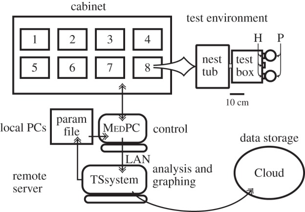
Schematic of the testing environment. Each fan-ventilated steel cabinet contains six to eight test environments. Each test environment consists of a polypropylene mouse tub connected via an acrylic tube to a Med Associates mouse test chamber with three hoppers (H) on the far wall. The two flanking hoppers have pellet feeders (P). (Adapted from [9].)

The protocols were implemented with MedPC code running on PCs in an adjacent room, which controlled the test environments and logged the data. The environment-control program wrote the data to a text file every 10 min. Data analysis and graphing software written using TSsystem, a custom open-source Matlab toolbox, harvested the data, analysed them and made graphic summaries three times a day. The evolving hierarchical data structure containing the raw data and the results derived from it, together with the evolving graphic summaries, were stored in ‘the Cloud’ and on in-laboratory computers by means of a commercial file-synchronization program. The data-analysing software decided when each mouse had completed a given protocol, based on user-specified criteria, and advanced it to the next protocol by writing to a text file of protocol parameter values, which was read every 10 min by the compiled MedPC program controlling an experimental environment.

The testing of the Bfc mice was terminated after 11 days by a storm-induced 5-day power failure. The testing of the L1 mice in the same environments was done subsequently; it went on without interruption for 86 days. The mice were not weighed during testing, because we adhered to the principle that they not be handled at all during testing. The protocols were run in the order in which they are discussed below. Because each mouse advanced automatically from protocol to protocol on the basis of simple performance statistics (e.g. for matching, the number of visit cycles completed), the duration of testing in each protocol varied widely from mouse to mouse.

4. The behavioural protocols

We tested the mice with three experimental protocols: the investment-to-income matching protocol, the instrumental- and classical-conditioning protocol and the timed-switching protocol. We were also able to test for circadian food anticipation in the L1 mice. We were not able to do this in the Batface mice owing to the 5-day power failure that terminated the testing of these mice.

(a). Investment-to-income ratio matching

In this protocol, which we call the matching protocol for short, the mouse obtains food pellets at two independent random rates by poking into two different hoppers. When it pokes into either hopper, it interrupts an infrared beam. If the protocol has armed the beam for a hopper, then interrupting it triggers the release of a pellet into that hopper. The two beams are armed on independent concurrently running variable-interval schedules of reinforcement: after each pellet delivery into a given hopper, a rearming interval for that hopper is drawn at random from an exponential distribution. Put another way, the arming intervals at the two hoppers are generated by independent Poisson processes. When an arming interval elapses, the beam for the hopper is rearmed. The next beam interruption delivers another pellet and restarts the Poisson process that will rearm that hopper's beam.

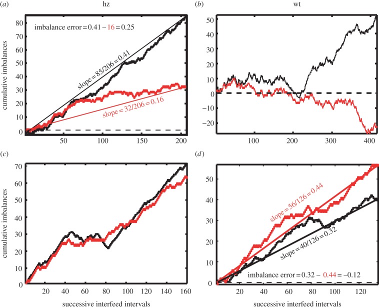
Like rats, pigeons and humans, mice tend to match the ratio of the average durations of their visits to the two hoppers—the ratio of their temporal investments in the two locations—to the ratio of the incomes obtained from those locations [31]. Income is the number of pellets per unit time—not per unit time spent at the hopper, but rather per unit time full stop. The extent to which a mouse is matching and the rapidity with which it adjusts its visit behaviour to accord with changes in the income ratio may be visualized by plotting on the same axes the pellet-by-pellet cumulative records of the income and investment imbalances (figure 2). The income imbalance is (F₁ − F₂)/(F₁ + F₂), where F_i is the number of pellets obtained from the ith hopper in a given interval. When computed on a pellet-by-pellet time scale, that is, at the end of each inter-pellet-delivery interval, this statistic takes on only the values +1 and −1, depending on whether the pellet delivery with which the interval ends is at hopper 1 or hopper 2, respectively. However, when the pellet-by-pellet values of this statistic are cumulated to make a cumulative record (cumulative income imbalance as a function of number of pellets obtained), then the slope of the cumulative record is the average imbalance. If, on average, the mouse obtains equal incomes from the two hoppers, then the slope is 0; if it obtains all of its income from hopper 1, then the slope is 1; if it obtains all of its income from hopper 2, the slope is −1; and if it obtains, say three out of every four pellets from hopper 1, the slope of the cumulative record is (1 + 1 + 1 − 1)/(1 + 1 + 1 + 1) = 0.75. Similarly, the investment imbalance statistic is (T₁ − T₂)/(T₁ + T₂), where T_i is the time spent at the ith hopper. For a single inter-pellet interval, it can take on any value on the interval [−1 1], but, as for the income imbalance statistic, the slope of the cumulative record of the income imbalance over any interval is the average imbalance over that interval. Thus, when the slopes of the two cumulative records are the same, the mouse is matching its investment imbalance to the income imbalance that it is experiencing (see figure 2 for four examples).

Figure 2.

Four examples of joint cumulative records of the pellet-by-pellet income (red plots) and the investment (black plots) imbalance statistics, two from heterozygotes (a,c) and two from littermate wild-type controls (b,d) for the two strains: (a,b) Batface and (c,d) L1. The mouse in (a) was overmatching; the mouse in (d) was undermatching. Note that the departures from matching in (a,b) occurred only over a portion of the records. In general, mice from this strain, whether wild-type or heterozygotes matched as well as those from the L1 strain. (Online version in colour.)

The imbalance statistic is a linear transformation of the more common Herrnstein fractions, which are F₁/(F₁ + F₂) and T₁/(T₁ + T₂). The difference between two average imbalances (two cumulative-record slopes) is twice the difference in the corresponding Herrnstein fractions. Thus, for example, when the slope of the income imbalance exceeds the slope of the investment imbalance by 0.2, the corresponding difference in the Herrnstein fractions—F₁/(F₁ + F₂) − T₁/(T₁ + T₂)—is 0.1. When the slope of the cumulative record of the investment imbalance is less extreme than that of the income imbalance, the mouse is undermatching; when it is more extreme, the mouse is overmatching. (See figure 2 for illustrations of this calculation.)

The matching protocol measures the accuracy with which a mouse can estimate two rates and compute their ratio. Because rate is number divided by time, this protocol also tests whether the mechanisms for estimating number and duration are intact. If the mouse could not remember which hopper produced which income, then it could not adjust the ratio of its visit durations to match the ratio of the incomes, so this protocol also tests the mouse's ability to remember a location and the events associated with that location. In other words, in addition to measuring the accuracy with which the mouse can estimate rates, the appearance of matching behaviour is evidence that the fundamental mechanisms of cognition that enable the animal to locate itself in space and time are intact. Finally, matching behaviour appears immediately: as soon as mice enter the test box and observe the rates at which they may obtain pellets from the two hoppers, they begin to match the ratio of their average visit durations to the ratio of the incomes they have observed [31]. It is hard to improve on this protocol when one wants a rapidly completed test of a broad range of basic cognitive functions. We put the mice into the environment completely naive; within 12 h we have good matching data for most mice. They give us important data while they are becoming accustomed to the environment.

(b). The instrumental- and classical-conditioning protocol

The rate of conditioning is often measured in behavioural work on the neurobiology of learning and memory. It is usually measured in a group of subjects by averaging trial-by-trial or block-of-trials by block-of-trials performance across subjects. The resulting group-average learning curve is generally concave downwards, and it may often be approximated by the cumulative exponential, the parameter of which may be taken as an estimate of the rate of learning. The problem with this method for measuring the rate of learning is that the relatively smooth concave downward curve is an artefact of the averaging. When the trial-by-trial performance of individual subjects is examined in most of the common animal learning paradigms, the conditioned response is commonly seen to appear in one or a few abrupt steps [32–34]. For examples of the abrupt appearance of classically conditioned hopper entry, see figure 4. The steps occur after different numbers of trials in different subjects, and they are of different heights, because some subjects show much more vigorous conditioned responding than do other subjects. Averaging across the steps in the individual records produces a function that seems to indicate an underlying process that obeys first-order kinetics (an exponential approach to asymptote), when in fact the underlying phenomenon, the transition for unconditioned to conditioned behaviour in a single subject, is discontinuous. Even when the transition in some subjects appears more or less continuous [35], it occurs after widely differing numbers of trials and over widely differing trial spans in different subjects within the same group. In such cases, averaging across the subjects in a group or condition produces a function whose mathematical form is not the same as the mathematical form of the function that describes the transitions in any one subject [36–38]. For example, the average across exponentials is not itself an exponential. For these reasons, the parameter(s) of a group-average learning curve are meaningless, except perhaps to students of animal sociology. Thus, in our combined instrumental- and classical-conditioning protocol, we measure trials-to-acquisition for each conditioned response in each subject.

Figure 4.

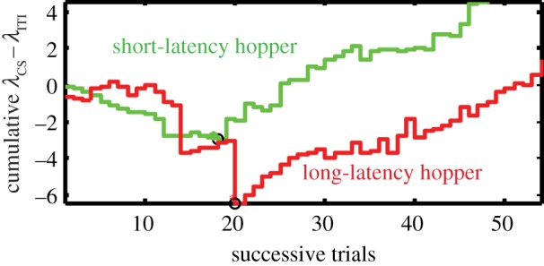
Illustrative cumulative records of the trial-by-trial difference between the rate of poking during the illumination of a flanking hopper (λ_CS) and the rate of poking into that same hopper during the intertrial interval (λ_ITI), when it is not illuminated and not about to deliver a pellet. Heavy dots mark the trials where the slopes reverse from negative to positive. The point at which this reversal occurs is our measure of trials-to-acquisition for the classically conditioned responses. (Online version in colour.)

In our protocol, there are three hoppers arranged along one wall of a standard MedAssociates mouse test chamber. When the middle hopper lights up, it signals to the mouse that it may initiate a simple sequence of events leading to the release of a pellet: when the mouse interrupts the infrared beam in the illuminated middle hopper, the light in that hopper goes off and one or the other flanking hopper illuminates. If it is the hopper on the left flank—the short-latency hopper—that illuminates, then a pellet is released into that hopper at the end of 4 s, regardless of what the mouse does. If it is the hopper on the right flank—the long-latency hopper—then the pellet is released into that hopper at the end of 12 s, again regardless of what the mouse does. Thus, the illumination of one or the other flanking hopper signals the release of a pellet into that hopper at the end of a hopper-specific delay.

In this protocol, the mouse's poking into the middle hopper initiates a simple sequence of events leading to reinforcement—the illumination of a flanking hopper followed at a fixed hopper-specific latency by the release of a pellet into that hopper. Because the poking is instrumental—no poke, no pellet—the emergence of trial-initiating pokes into the centre hopper is an instance of instrumental conditioning (also known as operant conditioning). On the other hand, once the trial has been initiated, a pellet is released into whichever flanking hopper illuminates regardless of what the mouse does. Thus, anticipatory poking into an illuminated flanking hopper (a conditioned hopper-entry response) is an instance of classical conditioning (also known as Pavlovian conditioning). Whether different learning mechanisms mediate the appearance of instrumentally conditioned and classically conditioned responses may be doubted [39], but it is commonly assumed that there are two different mechanisms [40]. If there are, and if it is possible to knock out the classical mechanism without knocking out the instrumental one, either genetically or pharmacologically, then one would observe mice that learned to initiate trials (instrumentally conditioned behaviour) but did not learn to poke into the illuminated flanking hopper in anticipation of a pellet release (classically conditioned behaviour).

If there are two conditioning mechanisms, then our protocol measures rate of acquisition for both. As in our matching protocol, we obtain our rate measures from cumulative records of trial-by-trial statistics. For instrumental conditioning, it is the cumulative record of trial-initiation speeds (figure 3a). For classical conditioning, it is the cumulative record of conditioned stimulus-intertrial interval (CS-ITI) poke rate differences (figure 4).

Figure 3.

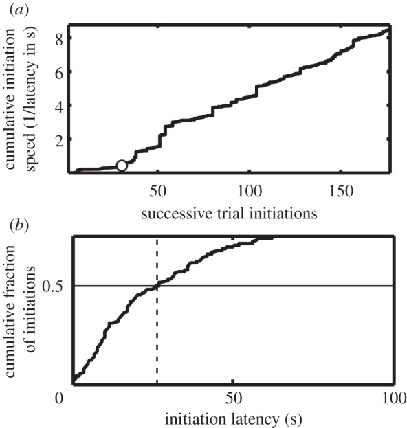
(a) Illustrative cumulative record of trial-initiation speed (speed = 1/latency in seconds). The open circle marks the trial at which the slope of the cumulative record increased, which we take to be the trial of acquisition for the instrumental response. (b) Illustrative cumulative distribution of trial-initiation latencies. The median latency (vertical dashed line) is the latency at which the horizontal solid line at 0.5 intersects the cumulative distribution. The distribution is truncated at 0.7, because the extremely long latencies at the tail of the distribution prevent the much shorter bulk of the distribution to be clearly seen.

The speed with which the mouse initiates a trial is the reciprocal of the latency of the trial-initiating poke. This latency is the interval between the illumination of the centre hopper and the beam interruption that signals the first post-illumination poke into that hopper. Because the mouse may be otherwise occupied or not even present (see description of the test environment below), very long trial-initiation latencies occur with some frequency. They dominate the cumulative record of the latencies. Taking reciprocals of these latencies to get trial-initiation speed rather than latency maps these atypically long latencies to essentially zero, with the desirable result that the much shorter and more typical trial-initiations dominate the cumulative record. When the mouse is slow to react to the illumination of the central hopper, the trial-initiation speeds are small. When it learns to initiate trials, the speeds increase, which produces a higher slope in the cumulative record of trial-initiation speeds (see figure 3a for an example). We take the trial at which the slope first shows a statistically significant increase to be the acquisition trial for the instrumental response (marked with an open circle in figure 3a). The first statistically significant increase was defined to be the first significant positive increment in average initiation speed that is greater than the average in the first segment when the cumulative record is segmented by the previously published CP_wrapper change-point-detecting function [32], using the Kolmogorov–Smirnov test, with a decision criterion equivalent to an alpha level of 0.01.

A measure of the vigour of instrumental performance is the median latency to initiate a trial (figure 3b). An effect of a genetic manipulation on this measure would generally be taken to indicate an effect on a performance variable rather than on a variable that mediates instrumental conditioning. When researchers rely on the group average learning curve, they often do not distinguish between effects on learning itself and effects on performance variables: both the change in the rate at which the curve approaches asymptote and the change in the asymptote are taken as changes in learning. This failure to distinguish effects on rate of learning from effects on performance is analogous to a failure to distinguish between competitive blockers and non-competitive blockers of molecular receptors in pharmacology and biochemistry. In both cases, the failure conflates changes in the location of the function from changes in its asymptote. In both cases, different mechanisms operate to determine location and asymptote.

The rate of poking into a flanking hopper during the interval when it is illuminated prior to a pellet release is the so-called CS response rate, that is, the rate of responding during the conditioned stimulus, which, in this case, is the illumination of the hopper into which the pellet will be released. The ITI rate is the rate of responding during the interval preceding the illumination of the centre hopper, which signalled the opportunity to initiate a trial. In other words, it is the rate of poking into the flanking hopper when it is not illuminated and there is therefore no prospect of an imminent pellet release there. Initially, before the mouse has learned that the illumination of a flanking hopper signals that a pellet release there is imminent, mice tend not to poke into an illuminated flanking hopper as frequently as they do during the ITIs when it is not illuminated. When this is true, the cumulative record of CS-ITI rate differences has a downward slope, because this difference is more often than not negative. Sooner or later, most mice begin to poke into an illuminated flanking hopper more frequently than into the same hopper when it is not illuminated. This reversal in the relative rates of poking is behavioural evidence that they have learned that the illumination of a flanking hopper signals the imminent release of a pellet there. When this reversal occurs, the slope of the cumulative record of CS-ITI rate differences becomes positive rather than negative (see figure 4 for examples). The trial on which the slope reverses is the acquisition trial for a classically conditioned response. Our protocol yields two such measures, one for the short-latency hopper and one for the long-latency hopper (figure 4).

(c). The timed-switching protocol

This protocol measures the accuracy and precision with which a mouse can measure and remember the durations of intervals. Fetterman & Killeen [41] first employed a version of it with pigeons as subjects. Balci et al. [42] adapted it for the mouse. It is similar to the protocol just described, except that when the mouse pokes into the illuminated trial-initiation hopper, both flanking hoppers illuminate (and, as in the previous protocol, the light in the centre hopper goes off). As in the previous protocol, on any trial, a pellet can be released into only one hopper. That is, on any trial, only one hopper is the ‘hot’ hopper, but the mouse has no means of knowing which. In this protocol, the pellet is released only in response to the first poke into the hot hopper at or after the delivery latency peculiar to it. Thus, when the short-latency flanking hopper is hot, a pellet is released in response to the first poke there at or after 4 s. When the long-latency flanking hopper is hot, a pellet is released there in response to the first poke at or after 12 s. If on a given trial, the first poke at or after the critical latency (4 or 12 s, depending on which hopper is hot) is into the wrong hopper (the ‘cold’ hopper), then the mouse loses its pellet. The erroneous poke terminates the trial, turning out the lights in both flanking hoppers, without the release of a pellet.

The rational thing to do on every trial in this protocol is to go first to the short-latency flanking hopper and poke there for the first 4 s. If it is a short-latency trial, poking there releases a pellet after 4 s. If a pellet is not released in response to pokes made at or after 4 s have elapsed, then the rational thing to do is to leave the short-latency flanking hopper and poke instead into the long-latency hopper on the other flank.

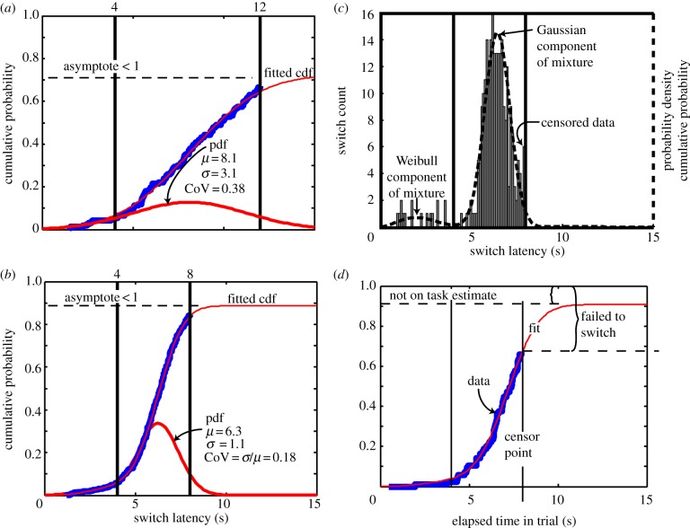
The latency to depart the short-latency hopper on a long-latency trial is a switch latency. In principle, the distribution of switch latencies might be thought to depend only on the duration of the short feeding latency (4 s). In fact, however, it depends on both this duration and the duration of the long feeding latency (12 s). These two feeding latencies are temporal goalposts. The mouse attempts to position its switch-latency distribution approximately optimally between these goalposts ([42,43]; figure 5a,b). Thus, the estimated mean (μ) of the distribution of switch latencies measures the accuracy with which the mouse can target the centre of the temporal goalposts, while the coefficient of variation (σ/μ) measures the precision with which it does so. (Accuracy is a measure of how close the central tendency of directed responses comes to an objective target; precision¹ is a measure of their dispersion about their central tendency. It is possible to be grossly inaccurate but highly precise and vice versa.) We begin with a 3 : 1 ratio between the short and long latencies (the goal posts). After at least 200 long trials (trials on which the mouse should switch), we shorten the long latency to 8 s and run the mouse for a minimum of another 200 long trials. For the mice with the L1 genotype, we ran two further blocks with at least 200 long trials, in which we shortened the longer delivery latency to 7 s and then to 6 s, keeping the shorter latency always at 4 s.

Figure 5.

Illustrative switch data with parameter-estimating fits. The thick blue curves in (a,b,d) are the empirical cumulative distribution of the observed switch latencies, that is, they are a plot of the raw data. The thin red lines superimposed on them are the best fitting six-parameter Weibull–Gauss functions. Five of these parameters are the parameters of a Weibull–Gauss mixture distribution, while the sixth parameter (asymptote) is an estimate of the fraction of the trials on which the mouse was on task (see §4c for explanation). The thicker red curve in (a,b) is the probability density distribution for the Weibull–Gauss mixture distribution with the same parameters as the cumulative distribution function (cdf) fitted to the cumulative data. It is an estimate of the probability density function (pdf) of the mouse's switch latencies. (a) From the first block of trials, when the feed latency at the long hopper was 12 s. (b) From the second block of switch trials, when the longer feed latency was reduced to 8 s. Reducing the longer feed latency, that is, bringing the temporal goalposts (vertical black lines) closer together, caused this and almost all other mice to increase the precision with which they timed their switches. It also shifted the mean of the Gaussian portion of the distribution leftward, keeping it more or less centred between the temporal goalposts. The solid vertical lines on each plot show the nominal short and long feed latencies, which we refer to as the temporal goalposts, because rational, goal-oriented switch latencies should fall within the interval they delimit. (c) Shows a switch-latency histogram, with counts plotted against left axis. Dashed curve is the fitted mixture distribution, plotted against the right (probability density) axis. The heavy vertical lines are the short (4 s) and long (8 s) feed latencies (the temporal goalposts). (d) To obtain a fit that accurately represents the observed steepness of the cumulative distribution, it is necessary to add an asymptote parameter that allows the cumulative distribution to asymptote below unity. If the fit function were required to asymptote at unity and to pass through the empirical censor point, it would either be too steep or too shallow. The amount by which the asymptote is estimated to fall short of unity is an estimate of the fraction of trials on which the mouse was not on task.

The switch latencies from a given subject in a given session tend to be bimodal [42,43]. There is an approximately Gaussian-distributed set of switches with mean near the optimal target switch latency. The second mode consists of switches that occur well before the short-latency pellet release (figure 5c). In these trials, the subject poked in the centre hopper to initiate a trial, poked in the short-latency hopper very briefly, and then quickly switched to the long-latency hopper. These quick departures (easily separable statistically from the typical, Gaussian-distributed timing behaviour) are not optimal—on short trials, they cost the mouse its pellet—so we refer to them as ‘impulsive switches’.

In some experiments, the impulsive switches have been best modelled by an exponential distribution [43], while in others they have been best modelled by a Weibull distribution [42]. Further work is required to tease apart the causes of these differences and their import. This is difficult because differences between the two models only become pronounced when the proportion of impulsive trials is large, and this is not often the case. We find that to fit the distributions obtained in the research we here report, we had to use the Weibull–Gauss mixture distribution, which has five parameters: the scale and shape parameters of the Weibull distribution, the mean and standard deviation of the Gaussian distribution and the proportion parameter which estimates the proportion of the switches attributable to the Weibull component.

Long trials, trials on which the subject should switch, automatically terminate if the subject is still poking into the short hopper when the long latency elapses. Thus, our switch times are censored at the longer feeding latency (figure 5c). We cannot record switch latencies longer than the longer delivery latency, so we do not know when the mouse would have switched on these censored long trials. We do, however, know the fraction of long trials on which they occur. A constraint on the distribution that we fit to the switch latencies is that it correctly predicts this fraction. Another constraint is that the steepness of the Gaussian component matches the steepness of the second rise in the observed cumulative distribution. The steepness of the second (and by far the greater) rise in the cumulative Weibull–Gauss mixture distribution is a function of the standard deviation of the Gaussian component. Our estimate of the precision of switch timing is the ratio between the estimated standard deviation of the Gaussian and the estimated mean of the Gaussian. Thus, systematic error in the estimation of the standard deviation leads to systematic error in the measure of precision.

We often find that the five-parameter Weibull–Gauss mixture distribution cannot simultaneously capture the fraction of switch trials on which the mouse fails to switch and the steepness of the Gaussian rise (see figure 5d for an example). A fit that accurately represents the steepness of the rise in the cumulative distribution of the observed switch latencies under-predicts the observed fraction of failures to switch. A fit that accurately predicts the observed fraction of failures to switch may grossly misrepresent the steepness of the rise in the Gaussian component of the observed distribution.

The problem arises from the fact that the algorithm for fitting a probability distribution to censored data assumes that the cumulative distribution asymptotes at unity, as do all cumulative distributions. In psychophysical work with human subjects, the empirical distributions often fail to asymptote at unity, because on some (usually small) fraction of the trials the subject is not on task. This creates empirical distributions with ‘fat tails’, also known as ‘outliers’. Thus, it is common to add an asymptote parameter, which allows the fitted distribution to come to an asymptote below unity. We follow that practice in fitting a Weibull–Gauss mixture distribution to our switch data. We add a sixth parameter that allows the fitted distribution to have an asymptote less than unity.

An asymptote parameter in psychophysical data fits is generally regarded as a necessary nuisance. That is what it is for us when we estimate the precision with which a mouse times its switches. In behavioural screening research, however, which is aimed at revealing the effects that a genetic or pharmacological manipulation may have on diverse underlying mechanisms of behaviour, the parameter may be of interest in its own right. Its additive inverse, 1 – A, where A is the estimated asymptote, measures the frequency with which a mouse is ‘not on task’ (figure 5d). A mouse may not be on task for a variety of reasons: it may, for example, have stopped to groom itself or left the test box for the nest-box and then returned much later to make another poke in the short hopper. Whatever the reason, it fails to time its switch to the longer hopper. For clinically oriented behavioural pharmacologists and the behavioural geneticists, this may be the measure of interest. For us, it is another way to assess the generality of the effects of a possibly deleterious genetic difference. Does the genetic difference cause the mice to be on task less often?

In summary, from the fitting of six-parameter Weibull–Gauss mixture distributions to switch latencies and failures to switch, we obtain four measures of interest: (i) the fraction of trials on which the mouse made an impulsive switch (a measure of impulsivity); (ii) the fraction of trials on which the mouse was not on task (a measure of distractibility); (iii) the Gaussian mean (a measure of the accuracy of interval timing) and (iv) the Gaussian coefficient of variation (σ/μ, a measure of the precision of interval timing).

(d). Circadian food anticipation

Animals of many kinds learn the phase of the circadian cycle at which events occur [1]. A simple manifestation of the mechanism that records and anticipates daily times of occurrence is the appearance of anticipatory activity in the few hours preceding the onset of one or more fixed phases of daily food availability [2,44–47]. To assess whether the mechanisms that enable the animal to record and anticipate circadian phase (time of day) were intact, we restricted the daily phases during which the above-described food-providing protocols were operative. A 4 h dusk food-availability phase began 1 h before the house light went off (dusk) and terminated 3 h after dusk. A 4 h dawn phase began 2 h before the house light came on (dawn) and terminated 2 h after dawn. Figure 6 is a representative daily raster plot (24 h actograph).

Figure 6.

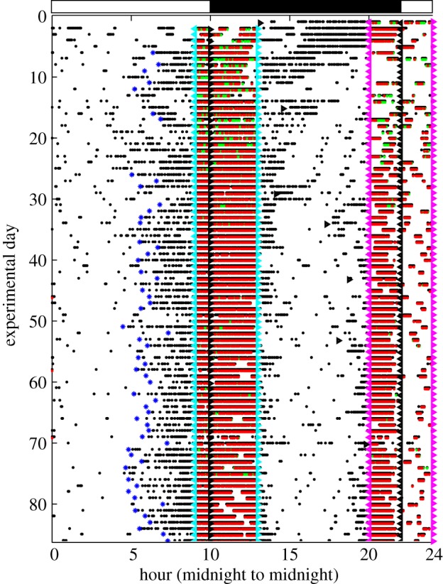
Representative 24 h actogram: raster plot of pokes (black dots) with one line per 24 h day. Cyan triangles with base to right mark the onset of the dusk feeding phase; base-left cyan triangles the offset; magenta triangles mark the onset and offset of the dawn feeding; black triangles mark house light on (dawn) and house light off (dusk). The light–dark cycle is also indicated by a bar at the top. Red and green dots mark pellet deliveries at the left and right hoppers, respectively. (Many green dots are overprinted with red dots.) The computed onsets of poking in anticipation of the onset of the dusk feeding phase are marked with large blue asterisks. Unambiguous anticipatory activity only occurs on some days. Those days become more frequent as testing progresses. The anticipatory activity is much more salient prior to the onset of the dusk feeding phase than prior to the dawn feeding phase. Feeding during the dawn phase often ceases abruptly when the house light comes on. All of these features are seen in most of the other 21 records from the testing of the L1 line, whether heterozygote or wild-type.

As is evident in the representative plot in figure 6, there is more feeding during the dusk feeding phase than during the dawn feeding phase, and there is much more prominent anticipatory activity preceding the dusk phase than the dawn phase. Therefore, we only compute measures of circadian anticipatory activity for the dusk phase. On any given day, we record the occurrence of activity anticipating the onset of the dusk feeding phase only if three-fourths of the behavioural events occur during the final one-third of the 9 h phase of no-food availability following the end of the dawn feeding phase and preceding the onset of the dusk feeding phase. This scoring treats the occurrence of anticipatory activity as an all or nothing event. Anticipatory activity thus scored does not occur during the first several days of testing. Our measure of ‘trials’ (days)-to-acquisition of circadian food-anticipatory activity is the day after which the frequency of anticipatory activity shows the first increase. The first positive change point in the probability of circadian anticipatory activity was computed using a Bayesian change-point finding algorithm (Jensen [48]), with the decision criterion on the Bayes factor in favour of a change versus no-change set to unity (even odds).

Our second measure of circadian anticipation is the time of onset of the anticipatory activity on those days on which it occurs (blue asterisks in figure 6). We compute this onset in the great majority of cases by locating the last inter-poke interval greater than 1 h and taking the end of that interval as the onset of the anticipatory poking activity. The algorithm is in the electronic supplementary material.

5. Results

(a). Matching

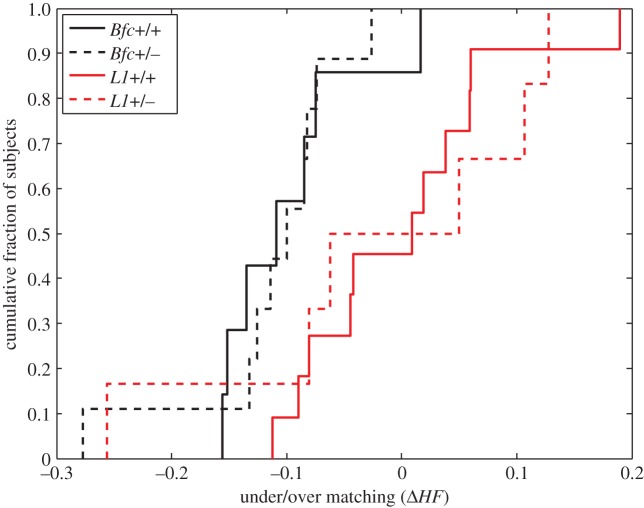
There were no genetic effects on the accuracy with which mice matched (figure 7). From this, we can conclude that many of the most basic cognitive mechanisms mediating learning and memory are intact. Mice heterozygous for the Batface mutation and for the L1 mutation can estimate number and duration and compute the ratio of these estimates to obtain an estimate of rate (income) and they can adjust the ratio of their average visit durations to match the ratio of the average incomes. For this to be possible, they must correctly associate their estimates of the incomes (rates of pellet delivery) to the locations. Thus, matching implies that they can distinguish spatial locations.

Figure 7.

Cumulative distributions of matching errors for wild-type and heterozygotic Bfc mice and for wild-type and heterozygotic L1 mice. signed as follows: if the proportion invested is more extreme than the income proportion, the sign is positive (overmatching); if the proportion invested is less extreme than the income proportion, the sign is negative (undermatching). There is no effect of genotype in either line, but the lines do appear to differ in their bias (toward undermatching, which is common), and in the magnitude of their errors. (Online version in colour.)

(b). Learning rates in basic conditioning paradigms

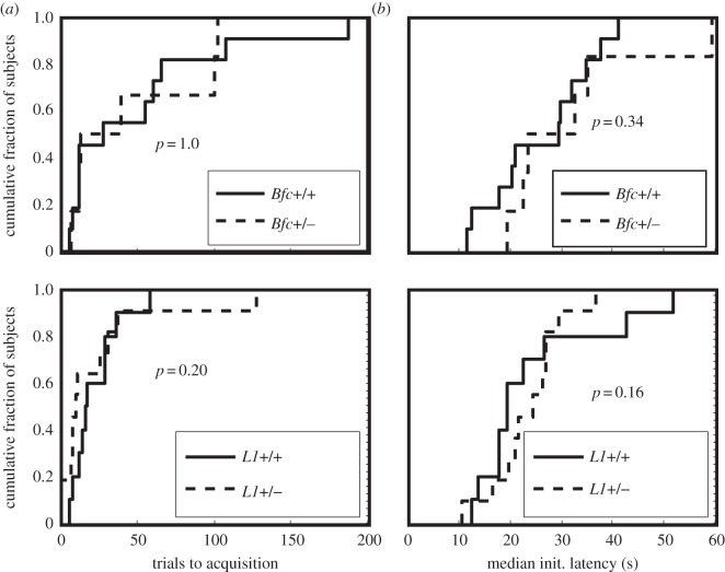
Both groups of heterozygous mice learned our instrumental task at the same rates as their wild-type littermate controls (figure 8a), and they initiated trials with the same latency once they had learned to do so (figure 8b).

Figure 8.

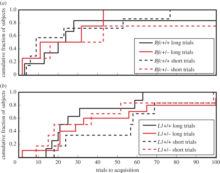
(a) Cumulative distributions of instrumental trials to acquisition for heterozygous Batface mutants (dotted line) and their wild-type littermate controls (solid line). The p-value is from the two-sample t-test for the difference in means. (b) Cumulative distributions of instrumental trials to acquisition for heterozygous L1 mutants (dotted line) and their wild-type littermate controls (solid line). The p-values are from a t-test for the difference in means between the +/+ and the +/− subjects.

The same is true for the rate of learning to anticipate food delivery in classically conditioned hopper entry (figure 9): there is no significant effect of genotype (+/+ versus +/mut or +/−) on trials to acquisition in either the Batface line or the L1 line. For both instrumental conditioning and classical conditioning, trials-to-acquisition measures vary by more than an order of magnitude within genotype, and some mice did not show anticipatory responding (classically conditioned hopper entry) within the span of the 250 trials that we put as the limit on this phase of the protocol. A large range of variation in trials to acquisition is commonly observed [32,34,49]. A measure that varies greatly between subjects drawn from highly inbred strains of laboratory animals may not be a promising measure from a genetic screening standpoint, because it is not under tight genetic control.

Figure 9.

(a,b) Cumulative distributions of trials to acquisition in the classically conditioned anticipatory hopper entry, as a function of genotype and short- versus long-duration of the conditioned stimulus (hopper illumination). The effects of genotype (+/+ versus +/mut or +/−) do not approach significance in either the Batface or the L1 lines. (Online version in colour.)

(c). Measures from the switch protocol

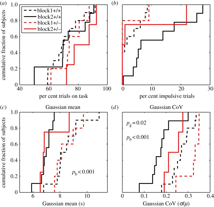
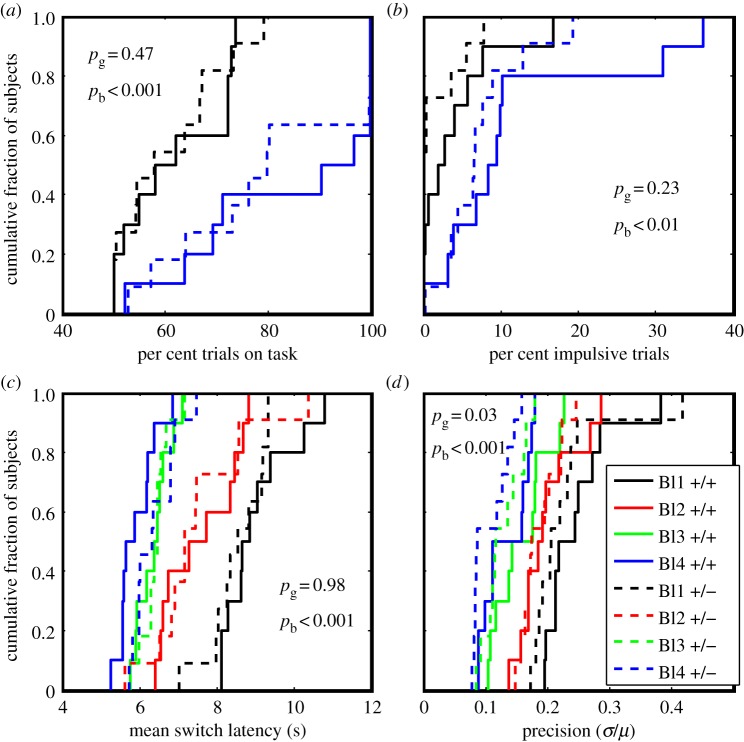
Figures 10 and 11 show the cumulative distributions of the four parameters of interest from fitting the Weibull–Gauss mixture distribution to the switch-latency data, as a function of trial block and genotype. Trials were run in blocks comprising at least 200 long trials, with the nominal pellet-delivery latency at the long-latency hopper reduced on successive blocks, from 12 to 8 to 7 to 6 s. Only blocks 1 (12 s) and 2 (8 s) were run with the Batface line.

Figure 10.

(a–d) Cumulative distributions of per cent trials on task, per cent impulsive trials, Gaussian mean switch latency and precision (CoV) in the Batface line, as a function of trial block and genotype. Difference in colour denotes difference in trial block (hence, in the nominal feed latency at the long hopper), while solid versus dashed denotes difference in genotype. The p-values (p_g for genotype and p_b for block) are for the main effects in two-way ANOVAs. The only main effect of genotype was on the precision with which switches were timed (bottom right plot): the heterozygotes were less precise. (Online version in colour.)

Figure 11.

(a–d) Cumulative distributions of per cent trials on task, per cent impulsive trials, Gaussian mean latency and the precision (CoV), in the L1 line, as a function of trial block and genotype. Difference in colour denotes difference in trial block, while solid versus dashed denotes difference in genotype. The p-values (p_g for genotype and p_b for trial block) are for the main effects in two-way ANOVAs. The interaction terms were in all cases insignificant. The only significant effect of genotype was on the precision with which trials were timed (bottom right plot): the heterozygotes were more precise.

Generally speaking, trial block (shortening the longer delivery latency) had an effect. It increased the per cent of trials on task. This may be simply an effect of increased experience with the task. Trial block also tended to increase impulsivity. This may well be because the difficulty of the task increased as the goalpost at the longer delivery latency moved closer to the goalpost at the shorter delivery. As expected, trial block had a strong effect on the Gaussian mean, the central tendency of the rationally timed switches. As the longer goalpost moved closer to the shorter, so did the central tendency of these switch latencies, keeping the Gaussian component of the mixture distribution approximately centred between the goalposts. Trial block also affected the precision of with which switches were timed: as the goalposts drew closer together, precision increased, which is to say that the coefficient of variation decreased. Put another way, the measured Weber fraction got smaller as the task grew more demanding.

(d). Circadian food anticipation

Figure 12 shows for the L1 mice line, the cumulative distributions of day of acquisition, mean onset hour for anticipatory activity within the 9 h interval preceding the onset of the dusk phase of food availability, and standard deviation of the onset hour. There was no effect of genotype on any of these measures. The testing of the Batface line was cut short by a prolonged power failure after 11 days, which was too soon to estimate the onset of anticipatory activity. (Note that the median onset day in the L1 line is 20, which is consistent with what we have observed in other strains.)

Figure 12.

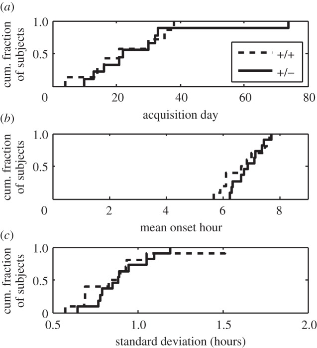
(a–c) Cumulative distributions of day of acquisition, mean onset hour and standard deviation of the onsets of food-anticipatory activity in the L1 line.

6. Discussion

The two genotypes Bfc(+/mut) and L1(female, +/−) have highly specific and opposing effects on the precision with which mice represent interval duration. The precision is reduced in the Bfc heterozygote, when compared with the wild-type control, and increased in the L1 heterozygote, when compared with the wild-type control. The functional specificity of these genetic effects is remarkable and important. Many other measures of learning, performance and cognition do not vary with these variations in genotype. These genotypic variations do not alter the rates of instrumental and classical conditioning. They do not alter the latency with which mice make an instrumentally conditioned response to the onset of a discriminative stimulus (the illumination of the central, trial-initiation hopper). They do not alter the accuracy with which mice match the ratio of their expected visit durations (their investment ratio) to the ratio of the incomes in a matching paradigm. They do not alter the accuracy with which mice adjust the mean of their switch-latency distribution to changes in the temporal goalposts that delimit the interval of rational switch latencies. And, in the L1 line at least, they do not alter the development of circadian food-anticipation, or the variability in the onset of this activity, or the length of the anticipatory interval (the interval between the onset of anticipatory activity and the onset of the anticipated phase of food availability). It will remain to be established how the behavioural phenotype of the heterozygous L1 mutant females relates to the observation that more neurons are generated and maintained in these mice when compared to their wild-type female littermates and the mutated male littermates. Thus, the histological phenotype of the heterozygous L1 knockout mutant is unexpectedly not intermediate between the wild-type and the homozygous mutant. This aspect together with the findings of the present—showing an improved functional parameter when compared with the wild-type littermates—deserves further investigations in humans carrying the L1 mutations in the heterozygous state, particularly in view of the notion that a surplus of neurons is not conducive to normal nervous system functions.

In short, the effect of these genetic variations is limited in its scope. We do not yet know how limited. It may be an effect on the precision with which quantities of all kinds are represented [50] or it may be specific to the representation of duration. To resolve that question, further behavioural testing is needed, including tests that assess the accuracy and precision of, for example, the representation of distance and direction in spatial tasks.

We also do not know whether these effects arise from the developmental effects of the genotypic variation or from the effects of the variations in the transcription of these genes in the adult brain. To determine that will require the development of facultative knockouts for these two genes. We also do not now know which altered physiological and/or neuroanatomical effects of these genotypic variations are responsible for the variation in the precision with which the mouse brain represents duration. That, too, must await the further investigation of these variations. The results we here report should motivate such investigations.

Forward behavioural genetics can play an important role in the establishment of linkage hypotheses [51], which is a central goal of behavioural and cognitive neuroscience [52–54]. It can best do so when behavioural screens target quantitative physiologically measurable properties of specific cognitive mechanisms. The precision with which a duration or any other simple magnitude, such as a distance, is represented in the brain is like the period of a behaviourally important intracellular biochemical oscillation (for example, the circadian clock) in that it can be measured both behaviourally and physiologically, that is, by electrophysiological, optical or by other biochemical or biophysical methods for measuring physiological variables.

Finally, we stress the importance for future investigations of the fully automated, highly quantitative approach to behavioural and cognitive genetics made possible by the system used to make the measures we have here described. The system produces a wealth of meaningful measures with very little human effort. The mice were never handled in the course of as many as 86 days of continuous testing. The 21 mice of the L1 line were run simultaneously. The number of mice that can be tested simultaneously is limited only by the number of test environments. Eight of the environments fit in a 1.22 × 0.61 × 1.98 m cabinet. The code that controls the testing protocols and the data-analysis code that derives the measures here reported are available from the senior author on request. The data-analysis code is written in a custom software Matlab toolbox, TSsystem, which greatly facilitates the creation of code that extracts complex behavioural structure from large scale databases consisting of time-stamped event records [9]. In the fully automated system, the data-analysis code is called automatically several times a day, providing the investigator with quasi-real-time graphic visualization of the progress of each mouse through the sequence of protocols, with summary statistics on each mouse, presented in graphic form.

The testing protocols and their application to these strains were approved by the Institutional Animal Care and Use Committee at Rutgers.

Funding statement

The behavioural research was supported by RO1MH077027 to C.R.G. The breeding of the Bfc mice was supported by Medical Research Council to P.M.N. The breeding and genotyping of the L1 mice was supported by the New Jersey Commission for Spinal Cord Research.

References

- 1.Gallistel CR. 1990. The organization of learning. Cambridge, MA: Bradford Books. [Google Scholar]
- 2.Luby M, Hsu C, Shuster S, Gallardo C, Mistlberger R, King OD, Steele AD. 2012. Food anticipatory activity behavior of mice across a wide range of circadian and non-circadian intervals. PLoS ONE 7, e37992 ( 10.1371/journal.pone.0037992) [DOI] [PMC free article] [PubMed] [Google Scholar]
- 3.Mistlberger RE. 1994. Circadian food-anticipatory activity: formal models and physiological mechanisms. Neurosci. Biobehav. Rev. 18, 171–195. ( 10.1016/0149-7634(94)90023-X) [DOI] [PubMed] [Google Scholar]
- 4.Weiner J. 1999. Time, love, memory: a great biologist and his quest for the origins of behavior. New York, NY: Alfred A. Knopf. [Google Scholar]
- 5.Konopka RJ, Benzer S. 1971. Clock mutants of Drosophila melanogaster. Proc. Natl Acad. Sci. USA 108, 2112–2116. ( 10.1073/pnas.68.9.2112) [DOI] [PMC free article] [PubMed] [Google Scholar]
- 6.Vitaterna MH, et al. 1994. Mutagenesis and mapping of a mouse gene, Clock, essential for circadian behavior. Science 264, 719–725. ( 10.1126/science.8171325) [DOI] [PMC free article] [PubMed] [Google Scholar]
- 7.Takahashi JS, Hoffman M. 1995. Molecular biological clocks. Am. Sci. 83, 158–165. [Google Scholar]
- 8.Kalsbeck A, Merrow M, Roenneberg T, Foster RG. (eds). 2012. The neurobiology of circadian timing. New York, NY: Elsevier. [DOI] [PubMed] [Google Scholar]
- 9.Gallistel CR, Balci F, Freestone D, Kheifets A, King AP. In press. Automated, quantitative cognitive/behavioral screening of mice: for genetics, pharmacology, animal cognition and undergraduate instruction. JoVE. [DOI] [PMC free article] [PubMed] [Google Scholar]
- 10.Maguschak KA, Ressler KJ. 2008. Beta-catenin is required for memory consolidation. Nat. Neurosci. 11, 1319–1326. ( 10.1038/nn.2198) [DOI] [PMC free article] [PubMed] [Google Scholar]
- 11.Maguschak KA, Ressler KJ. 2011. Wnt signaling in amygdala-dependent learning and memory. J. Neurosci. 31, 13 057–13 067. ( 10.1523/JNEUROSCI.3248-11.2011) [DOI] [PMC free article] [PubMed] [Google Scholar]
- 12.Maness PF, Schachner M. 2007. Neural recognition molecules of the immunoglobulin superfamily: signaling transducers of axon guidance and neuronal migration. Nat. Neurosci. 10, 19–26. ( 10.1038/nn1827) [DOI] [PubMed] [Google Scholar]
- 13.Salinas PC, Price SR. 2005. Cadherins and catenins in synapse development. Curr. Opin. Neurobiol. 15, 73–80. ( 10.1016/j.conb.2005.01.001) [DOI] [PubMed] [Google Scholar]
- 14.Murase S, Mosser E, Schuman EM. 2002. Depolarization drives beta-catenin into neuronal spines promoting changes in synaptic structure and function. Neuron 35, 91–105. ( 10.1016/S0896-6273(02)00764-X) [DOI] [PubMed] [Google Scholar]
- 15.Maguschak KA, Ressler KJ. 2012. The dynamic role of beta-catenin in synaptic plasticity. Neuropharmacology 62, 78–88. ( 10.1016/j.neuropharm.2011.08.032) [DOI] [PMC free article] [PubMed] [Google Scholar]
- 16.Nolan PM, et al. 2000. A systematic, genome-wide, phenotype-driven mutagenesis programme for gene function studies in the mouse. Nat. Genet. 25, 440–443. ( 10.1038/78140) [DOI] [PubMed] [Google Scholar]
- 17.Tucci V, et al. In preparation. Dominant mutations in human and mouse β-catenin lead to craniofacial dysmorphology and intellectual disability. [Google Scholar]
- 18.Moos M, Tacke R, Scherer H, Teplow D, Fruh K, Schachner M. 1988. Neural adhesion molecule L1 as a member of the 986 immunoglobulin superfamily with binding domains similar to 987 fibronectin. Nature 334, 701–703. ( 10.1038/334701a0) [DOI] [PubMed] [Google Scholar]
- 19.Hortsch M. 1996. The L1 family of neural cell adhesion molecules: old proteins performing new tricks. Neuron 17, 587–593. ( 10.1016/S0896-6273(00)80192-0) [DOI] [PubMed] [Google Scholar]
- 20.Maretzky T, Schulte M, Ludwig A, Rose-John S, Blobel C, Hartmann D, Altevogt P, Saftig P, Reiss K. 2005. L1 is sequentially processed by two differently activated metalloproteases and presenilin/gamma-secretase and regulates neural cell adhesion, cell migration, and neurite outgrowth. Mol. Cell. Biol. 25, 9040–9053. ( 10.1128/MCB.25.20.9040-9053.2005) [DOI] [PMC free article] [PubMed] [Google Scholar]
- 21.Hortsch M. 2000. Structural and functional evolution of the L1 family: are four adhesion molecules better than one? Mol. Cell. Neurosci. 15, 1–10. ( 10.1006/mcne.1999.0809) [DOI] [PubMed] [Google Scholar]
- 22.Brummendorf T, Kenwrick S, Rathjen FG. 1998. Neural cell recognition molecule L1: from cell biology to human hereditary brain malformations. Curr. Opin. Neurobiol. 8, 87–97. ( 10.1016/S0959-4388(98)80012-3) [DOI] [PubMed] [Google Scholar]
- 23.Fransen E, Lemmon V, Van Camp G, Vits L, Coucke P, Willems PJ. 1995. CRASH syndrome: clinical spectrum of corpus callosum hypoplasia, retardation, adducted thumbs, spastic paraparesis and hydrocephalus due to mutations in one single gene, L1. Eur. J. Hum. Genet. 3, 273–284. [DOI] [PubMed] [Google Scholar]
- 24.Dahme M, Bartsch U, Martini R, Anliker B, Schachner M, Mantei N. 1997. Disruption of the mouse L1 gene leads to malformations of the nervous system. Nat. Genet. 17, 346–349. ( 10.1038/ng1197-346) [DOI] [PubMed] [Google Scholar]
- 25.Law JW, Lee AY, Sun M, Nikonenko AG, Chung SK, Dityatev A, Schachner M, Morellini F. 2003. Decreased anxiety, altered place learning, and increased CA1 basal excitatory synaptic transmission in mice with conditional ablation of the neural cell adhesion molecule L1. J. Neurosci. 23, 10 419–10 432. [DOI] [PMC free article] [PubMed] [Google Scholar]
- 26.Migeon BR, Luo S, Jani M, Jeppesen P. 1994. The severe phenotype of females with tiny ring X chromosomes is associated with inability of these chromosomes to undergo X inactivation. Am. J. Hum. Genet. 55, 497–504. [PMC free article] [PubMed] [Google Scholar]
- 27.Lyon MF. 1961. Gene action in the X-chromosome of the mouse (Mus musculus L.). Nature 190, 372–373. ( 10.1038/190372a0) [DOI] [PubMed] [Google Scholar]
- 28.Rolf B, Kutsche M, Bartsch U. 2001. Severe hydrocephalus in L1-deficient mice. Brain Res. 891, 247–252. ( 10.1016/S0006-8993(00)03219-4) [DOI] [PubMed] [Google Scholar]
- 29.Guseva D, Angelov DN, Irintchev A, Schachner M. 2009. Ablation of adhesion molecule L1 in mice favours Schwann cell proliferaion and functional recovery after peripheral nerve injury. Brain Res. 132, 2180–2195. [DOI] [PubMed] [Google Scholar]
- 30.Schmid JS, Bernreuther C, Nikonenko AG, Ling Z, Mies G, Hossmann K-A, Jakovcevski I, Schachner M. 2012. Heterozygosity for the mutated X-chromosome-linked L1 cell adhesion molecule gene leads to increased numbers of neurons and enhanced metabolism in the forebrain of female carrier mice. Brain Struct. Funct. 218, 1375–1390. ( 10.1007/s00429-012-0463-9) [DOI] [PubMed] [Google Scholar]
- 31.Gallistel CR, King AP, Gottlieb D, Balci F, Papachristos EB, Szalecki M, Carbone KS. 2007. Is matching innate? J. Exp. Anal. Behav. 87, 161–199. ( 10.1901/jeab.2007.92-05) [DOI] [PMC free article] [PubMed] [Google Scholar]
- 32.Gallistel CR, Balsam PD, Fairhurst S. 2004. The learning curve: implications of a quantitative analysis. Proc. Natl Acad. Sci. USA 101, 13 124–13 131. ( 10.1073/pnas.0404965101) [DOI] [PMC free article] [PubMed] [Google Scholar]
- 33.Morris RW, Bouton ME. 2006. Effect of unconditioned stimulus magnitude on the emergence of conditioned responding. J. Exp. Psychol. Anim. Behav. Process. 32, 371–385. ( 10.1037/0097-7403.32.4.371) [DOI] [PubMed] [Google Scholar]
- 34.Papachristos EB, Gallistel CR. 2006. Autoshaped head poking in the mouse: a quantitative analysis of the learning curve. J. Exp. Anal. Behav. 85, 293–308. ( 10.1901/jeab.2006.71-05) [DOI] [PMC free article] [PubMed] [Google Scholar]
- 35.Harris JA. 2011. The acquisition of conditioned responding. J. Exp. Psychol. Anim. Behav. Process. 37, 151–164. ( 10.1037/a0021883) [DOI] [PubMed] [Google Scholar]
- 36.Estes WK. 1956. The problem of inference from curves based on group data. Psychol. Bull. 53, 134–140. ( 10.1037/h0045156) [DOI] [PubMed] [Google Scholar]
- 37.Estes WK. 2002. Traps in the route to models of memory and decisions. Psychon. Bull. Rev. 9, 3–25. ( 10.3758/BF03196254) [DOI] [PubMed] [Google Scholar]
- 38.Estes WK, Maddox WT. 2005. Risks of drawing inferences about cognitive processes from model fits to individual versus average performance. Psychon. Bull. Rev. 12, 403–409. ( 10.3758/BF03193784) [DOI] [PubMed] [Google Scholar]
- 39.Gallistel CR, Gibbon J. 2000. Time, rate, and conditioning. Psychol. Rev. 107, 289–344. ( 10.1037/0033-295X.107.2.289) [DOI] [PubMed] [Google Scholar]
- 40.Domjan M. (ed.). 2003. The principles of learning and behaviour. Belmont, CA: Thomson. [Google Scholar]
- 41.Fetterman JG, Killeen PR. 1995. Categorical scaling of time: implications for clock-counter models. J. Exp. Psychol. Anim. Behav. Process. 21, 43–63. ( 10.1037/0097-7403.21.1.43) [DOI] [PubMed] [Google Scholar]
- 42.Balci F, Freestone D, Gallistel CR. 2009. Risk assessment in man and mouse. Proc. Natl Acad. Sci. USA 106, 2459–2463. ( 10.1073/pnas.0812709106) [DOI] [PMC free article] [PubMed] [Google Scholar]
- 43.Kheifets A, Gallistel CR. 2012. Mice take calculated risks. Proc. Natl Acad. Sci. USA 109, 8776–8779. ( 10.1073/pnas.1205131109) [DOI] [PMC free article] [PubMed] [Google Scholar]
- 44.Bolles RC, Moot SA. 1973. The rat's anticipation of two meals a day. J. Comp. Physiol. Psychol. 83, 510–514. ( 10.1037/h0034666) [DOI] [PubMed] [Google Scholar]
- 45.Edmonds SC, Adler NT. 1977. The multiplicity of biological oscillators in the control of circadian running activity in the rat. Physiol. Behav. 18, 921–930. ( 10.1016/0031-9384(77)90202-5) [DOI] [PubMed] [Google Scholar]
- 46.Rosenwasser AM, Pelchat RJ, Adler NT. 1984. Memory for feeding time: possible dependence on coupled circadian oscillators. Physiol. Behav. 32, 25–30. ( 10.1016/0031-9384(84)90064-7) [DOI] [PubMed] [Google Scholar]
- 47.Mendoza J, Albrecht U, Challet E. 2010. Behavioural food anticipation in clock genes deficient mice: confirming old phenotypes, describing new phenotypes. Genes Brain Behav. 9, 467–477. [DOI] [PubMed] [Google Scholar]
- 48.Jensen G. 2013. Closed-form estimation of multiple change-point models. PeerJ PrePrints 1, e90v2 ( 10.7287/peerj.preprints.90v2) [DOI] [Google Scholar]
- 49.Ward RD, Gallistel CR, Jensen G, Richards VL, Fairhurst S, Balsam PD. 2012. Conditional stimulus informativeness governs conditioned stimulus–unconditioned stimulus associability. J. Exp. Psychol. Anim. Behav. Process. 38, 217–232. ( 10.1037/a0027621) [DOI] [PMC free article] [PubMed] [Google Scholar]
- 50.Gallistel CR. 2011. Mental magnitudes. In Space, time and number in the brain: searching for the foundations of mathematical thought (eds Dehaene S, Brannon L.), pp. 3–12. New York, NY: Elsevier. [Google Scholar]
- 51.Sharpe L, Stockman A, Jägle H, Nathans J. 1999. Opsin genes, cone photopigments, color vision and color blindness. In Color vision: from genes to perception (eds Gegenfurtner K, Sharpe L.), pp. 3–52. New York, NY: Cambridge University Press. [Google Scholar]
- 52.Gallistel CR, Shizgal P, Yeomans JS. 1981. A portrait of the substrate for self-stimulation. Psychol. Rev. 88, 228–273. ( 10.1037/0033-295X.88.3.228) [DOI] [PubMed] [Google Scholar]
- 53.Teller DY. 1984. Linking propositions. Vis. Res. 24, 1233–1246. ( 10.1016/0042-6989(84)90178-0) [DOI] [PubMed] [Google Scholar]
- 54.Tsien JZ. 2000. Linking Hebb's coincidence-detection to memory formation. Curr. Opin. Neurobiol. 10, 266–273. ( 10.1016/S0959-4388(00)00070-2) [DOI] [PubMed] [Google Scholar]