Singular Hopf bifurcation in a differential equation with large state-dependent delay

Abstract

We study the onset of sustained oscillations in a classical state-dependent delay (SDD) differential equation inspired by control theory. Owing to the large delays considered, the Hopf bifurcation is singular and the oscillations rapidly acquire a sawtooth profile past the instability threshold. Using asymptotic techniques, we explicitly capture the gradual change from nearly sinusoidal to sawtooth oscillations. The dependence of the delay on the solution can be either linear or nonlinear, with at least quadratic dependence. In the former case, an asymptotic connection is made with the Rayleigh oscillator. In the latter, van der Pol’s equation is derived for the small-amplitude oscillations. SDD differential equations are currently the subject of intense research in order to establish or amend general theorems valid for constant-delay differential equation, but explicit analytical construction of solutions are rare. This paper illustrates the use of singular perturbation techniques and the unusual way in which solvability conditions can arise for SDD problems with large delays.

1. Introduction

State-dependent delays (SDDs) are a common occurrence in natural or artificial systems subjected to feedback. In motion control, for instance, the delay of a signal reflected by an obstacle depends on the current position of the vehicle [1]. Another well-documented area of research where SDD problems are formulated concerns chatter instabilities. In cutting processes and in milling or rotary drilling systems used by oil industries, SDDs arise owing to the deformation of the cutting tool [2–4]. Furthermore, in population dynamics, the time required for the maturation level of a cell to achieve a certain threshold can be modelled as an SDD [5–7]. Finally, the electromagnetic two-body problem stands as a fundamental SDD problem in physics which has been regularly revisited over the years [8–11]. The mathematical analysis of SDD problems is still fairly recent compared to constant-delay differential equations and requires the development of new theoretical [12] and numerical [13] tools.

Some of these SDD models differ considerably from others, and most of them do not look simple (see the review by Hartung et al. [12]). In [2–5,14,15], the delay is not given explicitly as a function of the state variables but is defined implicitly by an integral equation that needs to be solved together with the remaining equations. The large diversity of SDD equations is such that a general theory is still lacking. This is why simple-looking equations are studied in detail as reference problems. In this work, we focus on one such problem, namely the scalar SDD equation

1.1

where k>0 is our control parameter and ε≪1 is a small parameter. More precisely, we will study the first Hopf bifurcation of the trivial solution x=0 as k is varied. A general Hopf theorem, stipulating the conditions under which a periodic solution bifurcates from a steady state was only established very recently [16–18]. In this work, we construct explicitly the periodic solution of equation (1.1) in the weakly nonlinear limit of small x, taking advantage of the smallness of ε. Asymptotic treatments of this kind appear to be lacking in the literature of SDD differential equation and could thus be a useful complement to the rigorous theories that are being developed. Most of this paper is devoted to the simple SDD

1.2

The more general case

1.3

turns out to require a separate treatment and is treated at a second stage. Recently, a local bifurcation technique was applied to a weakly damped nonlinear oscillator, showing how the functional form of an SDD influences the direction of bifurcation [19]. Equation (1.1) with the linear SDD given by (1.2) has been intensively studied by John Mallet-Paret and Roger Nussbaum during the last 20 years [20–23] in order to develop analytical techniques that exploit the smallness of ε. Recently, an extension of this equation to the case of two SDDs was studied by Humphries et al. [24].

Taken with a constant delay, equation (1.1) is well documented in the control literature where the stabilization of the system

1.4

is investigated with the control law u(t)=Kx(t) and for all possible values of a and K [25]. When the delay is state-dependent, the basic steady state x=0 and its stability properties remain unchanged but the problem is now violently nonlinear. Regarding (1.1) in the light of (1.4), ε can be interpreted as the ratio between the intrinsic dynamical time scale of the system (when u=0) and the delay of the control. Thus, ε≪1 stands as a large-delay limit.

Equation (1.1) displays a Hopf bifurcation at some value k=k_H(ε) but, as we shall demonstrate, this bifurcation is singular in the limit ε→0. Specifically, the small-amplitude expansion of the periodic solution in powers of (k−k_H)^1/2 becomes non-uniform as ε→0, making the Hopf bifurcation singular. Following the method of matched asymptotic expansions [26–28], a new asymptotic expansion of the solution where k−k_H is properly scaled with respect to ε is then considered as a separate perturbation problem. This approximation is connected to the first Hopf approximation through a process called ‘matching’ so that both solutions overlap. Specific singular Hopf bifurcation problems have been analysed in detail for neuronal and laser bifurcation problems [29–32] and for a constant-delay differential equation problem modelling high-speed machining [33]. A distinctive feature of the present problem from these earlier examples of singular Hopf bifurcation is that the second asymptotic expansion itself rapidly loses its validity with increasing k−k_H. Therefore, a third asymptotic expansion becomes necessary. Let us remark that Hopf bifurcations for slow–fast systems with one fast and two slow variables were studied in detail by Guckenheimer and co-workers [34,35]. In these references, the definition of a singular Hopf bifurcation is geometrical and is related to the observation of fold points of critical manifolds.

Mallet-Paret & Nussbaum [20] showed that the solution of equation (1.1) approaches a sawtooth limiting profile as ε→0 with k>1. Figure 1 shows a numerical example. The period of the oscillations is close to the value k+1, and the leading approximations of the extrema are

1.5

A numerical bifurcation diagram of the periodic solutions is shown in figure 2 where the upper and lower straight lines are provided by (1.5). The parabolic curve emerging from x=0 in the vicinity of k=1 comes from a local Hopf calculation, which we provide here. The bifurcation diagram in figure 2 indicates that the branch of periodic solutions emerges from a Hopf bifurcation and that the extrema of the oscillations gradually increases until they approach the lines and corresponding to the fully developed sawtooth oscillations. A close examination of the oscillations near the Hopf bifurcation reveals that the transition from sinusoidal to sawtooth oscillations is very rapid as one gradually increases k from k_H (figure 3). In this paper, we show that the Hopf bifurcation becomes progressively more vertical near k=k_H as ε→0. The oscillations are nearly sinusoidal in the domain k−k_H=O(ε⁴) but change from sinusoidal to sawtooth as soon as k−k_H=O(ε²) for the linear SDD (1.2). On the other hand, sawtooth oscillations appear at k−k_H=O(ε) for the general SDD (1.3). By contrast to the previously mentioned singular Hopf bifurcation problems, the problem with SDD (1.2) requires the solution of two inner problems that result from two successive singularities in the perturbation expansions. Eventually, the transition from sinusoidal to sawtooth oscillations is captured by Rayleigh’s nonlinear ordinary differential equation. For the general case SDD (1.3), we find that the oscillations are described by van der Pol’s equation.

Figure 1.

Sawtooth oscillations with equations (1.1) and (1.2), integrated numerically with k=1.5 and ε=0.05.

Figure 2.

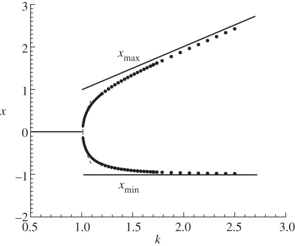
Bifurcation diagram of the periodic solutions (ε=0.05). The dashed line represents the local approximation y=±2δ where δ is given by (3.11). The two solid lines are the asymptotic approximations of the sawtooth oscillations given in (1.5).

Figure 3.

Periodic solutions close to the Hopf bifurcation (ε=0.05). They have been obtained numerically from equation (1.1). The value of k is indicated in the figure. (Online version in colour.)

For nonlinear constant delay equations, the method of linearization is a standard tool in stability and bifurcation studies. But for SDD equations, this approach is delicate because the solution of the system is not differentiable with respect to the SDD [36]. Cooke & Huang [37] first addressed the question of the local stability of a constant equilibrium. Under reasonable assumptions, the formal linearization where the delay is evaluated at steady state does reflect the stability of the steady state of the SDD.

The rest of the paper is organized as follows. In §2, the linear stability analysis is briefly reviewed and some scalings are anticipated. Section 3 contains a first, textbook type, local analysis of the Hopf bifurcation point when the SDD is given by (1.2). Its validity is seen to break down already as k−k_H becomes O(ε⁴). This is the limit studied in §4, where a corrected relationship between the oscillation amplitude and k−k_H is derived. However, a second breakdown of the analysis is found, which motivates the investigation of a new limit, k−k_H=O(ε²) in §5. Section 6 relates the small amplitudes oscillations to those of Rayleigh’s oscillator. In §7, the general SDD (1.3) is studied, eventually leading to a description of oscillations with van der Pol’s equation. Finally, we comment on how different types of solvability conditions sequentially lead to informations on the solutions. We also discuss the interest of exploring singularly perturbed SDD problems.

2. Preliminaries

Equation (1.1) admits the steady state x=0 and is linearized simply by setting τ=1. In this linearized equation, solutions of the form , with real ω, exist at the Hopf bifurcation points k_n(ε) and Hopf bifurcation frequencies ω_n(ε) given by

2.1

Assuming k>0, we have, as ε→0,

2.2

We note that these bifurcation points become infinitely close as ε→0 (figure 4). Let us denote the smallest bifurcation point, k₀, and corresponding frequency, ω₀, by k_H and ω_H, respectively. They have the following asymptotic expression:

2.3

and

2.4

It is that bifurcation point which is responsible for the change of stability of the solution x=0.

Figure 4.

Hopf bifurcation lines, from equation (2.2).

In this paper, we perform a local analysis to study the amplitude and shape of the periodic solutions as a function of k−k_H(ε). From the linear stability analysis above, one may anticipate that the presence of the bifurcation points k₁,k₂,…, will be felt as soon as k−k_H=O(ε²), so that the standard analysis has to be revised at this point. However, the standard analysis turns out to break down much earlier, yielding a first distinguished limit when k−k_H=O(ε⁴). Then, a second distinguished limit is found for k−k_H=O(ε²), where all the frequencies ω_n appear in the leading order solution. In this way, a scenario for the transition from harmonic to sawtooth oscillation is emerging.

3. Regular Hopf bifurcation (k−k₀≪ε⁴)

The construction of the periodic solutions of equations (1.1) and (1.2) bifurcating from the trivial solution x=0 initially follows a standard pattern [38]. We first introduce the time s≡σt, in which x(s) is 2π-periodic, and the small amplitude

3.1

In the rescaled time, equations (1.1) and (1.2) become

3.2

The solution as well as σ is then found by using the expansion

3.3

3.4

and

3.5

where we have anticipated from Hopf bifurcation theorem that the expansion of k and ω admits no odd power corrections in δ. Inserting (3.3)–(3.5) into equation (1.1) and equating to zero the coefficients of each power of δ, we obtain a sequence of linear problems for the unknown functions x_i(s). They are of the form

3.6

where the right-hand-side H_m is a function involving the solutions at the previous orders only. Given from the linear stability analysis that

3.7

the solvability conditions of (3.6) is that the right-hand sides H_m contain no term proportional to . These conditions will provide the unknown coefficients κ₂ and σ₂.

From the analysis of the three first problems, we find that the final solution has the form

3.8

where c.c. means complex conjugate and p₀, p₂, p₃ are constants depending on ε. In the limit ε→0, they are given by

3.9

while κ₂ and σ₂ are given by

3.10

Using (3.4) and the expression of κ₂ in (3.10), we determine δ as a function of the deviation k−k_H. We obtain

3.11

We next note from (3.9) that p₃∝ε⁻¹. As a result, expansion (3.3) loses its asymptotic character as soon as

3.12

since the second- and third-order terms become of comparable size. Combining (3.12) and (3.11), the breakdown of the present analysis occurs when

3.13

where α=O(1). Let us examine the limiting behaviour of expression (3.8) when (3.13) is assumed:

3.14

This will be used as a matching condition when we develop a new expansion of the solution. The corresponding limiting expression for the frequency. Using (3.5), (3.10), (3.11) and (3.13), we find

3.15

indicating that the first correction of the frequency coming from the nonlinear problem is proportional to ε³.

In summary, we have found that the standard Hopf asymptotic approximation is valid only if k−k_H≪ε⁴. If k−k_H∼ε⁴α, a new expansion of the solution is needed where we use ε as the small parameter. As we shall see in §4, the new solution remains sinusoidal but its amplitude changes dramatically from a (k−k_H)^1/2 scaling law to an (k−k_H)^1/4 dependence.

4. Singular Hopf bifurcation (k−k_H=ε⁴α)

Solution (3.14) suggests to seek a solution in powers of ε. We try the expansion

4.1

4.2

and

4.3

where s≡σt and x(s,ε) is 2π-periodic in s. As suggested by (3.13) and (3.15), we assume that the first corrections of k and σ that contribute to the nonlinear problem are ε⁴ and ε³, respectively. Inserting (4.1)–(4.3), we now obtain at each order in ε a problem of the form

4.4

where H_m(s) is computed from the previous orders. The decomposition of the perturbation problem into a series of iterative maps is typical of delay differential equations with large delays [38–41]. Rewriting the above equation at time s−π and using the fact that x_m(s−2π)=x_m(s), we obtain

4.5

Substracting (4.5) from (4.4) then yields the solvability condition for the right-hand side H_m

4.6

The existence of such a solvability condition originates from the fact that the homogeneous problem w(s)+w(s−π)=0 admits non-trivial 2π-periodic solutions. Indeed, any combination of harmonic functions with j odd makes the left-hand side of (4.4) vanish. The general solution of the problem (4.4) under the condition (4.6) is given by

4.7

Expressions (4.6) and (4.7) can be used to implement an automatic resolution of the perturbation analysis up to any order using a symbolic software such as Mathematica.¹

At first order, we have

4.8

At second order, the right-hand side is

4.9

Next, we obtain

4.10

With H₃(s), a first non-trivial solvability condition is obtained, which yields the profile of W₁(s)

4.11

At fourth order, a new solvability condition determines W₂(s)

4.12

However, in order to prevent secular divergence of W₂, a secondary solvability condition, this time on equation (4.12), must be satisfied

4.13

giving the first nonlinear correction to the frequency. Thus, , giving

4.14

Finally, at fifth order, the solvability condition is a differential equation for W₃

4.15

where

4.16

As before, the solvability condition on equation (4.15) is that q₁ vanishes, eventually providing the relationship between the solution amplitude and the deviation from the Hopf bifurcation point:

4.17

In summary, we found that

4.18

where

4.19

and

4.20

Our solution is valid provided it matches (3.14) in the limit A→0. In this limit, we note from (4.19) that

4.21

or equivalently with (3.13),

4.22

With (4.22), we verify that expression (4.18) is exactly matching expression (3.14). We next examine the behaviour of solution (4.18) as the amplitude A increases. Specifically, we note that the expansion of the solution becomes itself non-uniform as the second term in the coefficient of ε² becomes comparable with the leading term in ε. This occurs when

4.23

Using (4.23), we note from (4.19) that the leading expression for k−k_H now is

4.24

which implies that k−k_H=O(ε²). Introducing

4.25

the solution of (4.19) now has the approximation

4.26

With (4.26), our expression (4.19) becomes

4.27

It suggests to seek a new solution now in powers of ε^1/2. Finally, using (4.20) and (4.23), we determine the frequency as

4.28

In summary, the analysis of the solution in critical domain (3.13) indicates that the periodic solution remains nearly sinusoidal but that the amplitude of the oscillations, after the initial (k−k_H)^1/2 law, subsequently levels off as (k−k_H)^1/4 (figure 5).

Figure 5.

Bifurcation diagram representing as a function of k (ε=0.05). It shows the progressive transition from to as k−k_H increases from zero. (1) the amplitude A is determined from equation (4.19); (2) the small amplitude limit is given by (4.21); (3) the large amplitude limit is given by (4.24). (Online version in colour.)

5. Singular Hopf bifurcation (k−k_H=ε²β)

Limiting expressions (4.25), (4.27) and (4.28) motivate the new expansion

5.1

5.2

and

5.3

where s=σt and x(s) is 2π−periodic in s. Inserting (5.1)–(5.3) into equation (3.2) and equating to zero the coefficients of each power of ε^1/2, we obtain a new sequence of linear problems for the unknown functions x₁, x₂, x₃,…. They are of the form (4.4) and their resolution follows from (4.7) as in §4. We obtain, successively, for the first four orders,

5.4

5.5

5.6

and

5.7

The above right-hand sides are all even in s and therefore automatically satisfy solvability condition (4.6). The first non-trivial solvability condition arises at O(ε^5/2) and reads, with x₁(s)=W₁(s),

5.8

Hence, the leading-order solution is no more sinusoidal but contains an arbitrary number of harmonics, as anticipated in the Introduction. We have to solve equation (5.8) with the condition

5.9

This provides a necessary relationship between σ₄ and κ₄. To be valid, x₁(s)=W₁(s) must match expression (4.25) in the small amplitude limit. To this end, we solve (5.8) in the small-amplitude limit. Introducing a new small parameter η≪1, we thus write

5.10

and

5.11

where we have omitted all zero contributions for clarity. From the analysis of the problems for w₁, w₃ and w₅, and their solvability conditions, equation (5.8) eventually yields

5.12

From the expression of κ₄ in (5.12) and (5.2), we determine η as

5.13

which we recognize as parameter a in (4.26). Hence, the small-amplitude limit (5.12) of approximate solution (5.1) matches the large-amplitude limit, (4.27), of previous expansion (4.1).

We have thus found that the oscillations are changing from nearly linear to nonlinear in the critical domain (4.25). In §6, we analyse these nonlinear oscillations.

6. Rayleigh’s equation

Equation (5.8) is nonlinear and is the final problem of our singular Hopf bifurcation analysis. This equation can be reformulated in a more meaningful form by introducing the new variables (σ₄<0)

6.1

and

6.2

Indeed, in terms of y and T, equation (5.8) can be recognized as Rayleigh’s equation [26,42]

6.3

where prime means differentiation with respect to time T. The only parameter left, Λ, is defined by

6.4

For any initial condition, the solution approaches a stable limit-cycle of period P. Note that the change of sign in T is necessary in order to have a stable limit-cycle of equation (6.3). Given Λ, we determine the period P numerically. The corresponding period in s must be 2π which implies, using (6.2), that

6.5

From this, we extract κ₄ as

6.6

Combining (6.6) with (6.4) and (6.1), we further obtain

6.7

Of particular interest is the asymptotic behaviour of the solution as , corresponding to in (6.3). The solution to that problem is well documented (see, for instance [26,42]) and gives, for the leading expressions of P and the extrema of y

6.8

Using (6.6) and (6.7), the corresponding values for κ₄ and x₁ are

6.9

The resulting analytical bifurcation diagram and time traces are compared to numerical simulations in figures 6 and 7. A good quantitative agreement is seen as long as ε is sufficiently small and k is close to 1. As k increases, however, the shape of the oscillations differ more and more between the original model and the asymptotic reduction. Indeed, the descending part of the oscillations become more and more vertical in the original model (1.1) (figure 1) which the Rayleigh oscillator cannot reproduce.

Figure 6.

Bifurcation diagram for x and , as functions of k. It shows the gradual change from to a new (k−k_H)^1/2 scaling law provided by the solution of Rayleigh’s equation. The extrema of x₁ have been obtained numerically from equation (6.3) for 0<Λ<10 (Line 1). Line 3 is the local approximation provided by (5.13). Line 2 is the large Λ approximation given by (6.9). (Online version in colour.)

Figure 7.

Comparison between numerical solutions of original equation (1.1) (solid line) and its Rayleigh asymptotic reduction (5.8) (dashed line) for two values of ε. (Online version in colour.)

7. More general state-dependent delays

We now consider general SDDs. Expanding τ(x) in Taylor series, we may write, in all generality

7.1

provided that τ′(0)>0. Given that x is small, higher order terms in (7.1) can be neglected in this analysis. It would seem at first that the quadratic term above should lead only to a small correction to the preceding results. Its influence on the dynamics, however, turns out to be predominant. Indeed, performing the same analysis as in §3, that is with an asymptotic development of the form (3.3)–(3.5), the expressions in (3.10) eventually become

7.2

Hence, in the small-ε limit, the direction of bifurcation, given by the sign of κ₂, is entirely dictated by b (assuming that it is O(1)). In particular, b must be negative for the bifurcation to be supercritical. A similar observation was made by Mitchell & Carr [19] in their study of a weakly damped nonlinear oscillator with SDD. On the other hand, (3.11) is now

7.3

while the solution has the asymptotic form

7.4

Thus, the second- and third-order terms become of the same magnitude as soon as δ=O(ε²). On the other hand, the third and fundamental harmonics balance when δ=O(ε). Let us focus directly on the latter case. The analysis of the singular Hopf bifurcation problem now requires an expansion of x(s) in power of ε

7.5

where the x_j(s) are 2π−periodic functions of s defined by

7.6

We also need to expand the bifurcation parameter as

7.7

Substituting this development in (1.1) with τ given by (7.1), the first two problems arising at O(ε) and O(ε²) are exactly as in §4. At the next order, the solvability condition reads

7.8

Together with the periodicity condition x₁(s+2π)=x₁(s). Equation (7.8) is van der Pol’s equation. Indeed, with and , equation (7.8) becomes

7.9

where prime means differentiation with respect to time T. Following the same reasoning as before, a solution of period P in T must be of period 2π in s, giving κ₂=(P²−4π²)/8 and σ₂=πPΛ/4. A comparison between numerical simulations of equation (1.1) and its van der Pol asymptotic reduction is given in figure 8 for ε=0.05. The similarity of the shape of oscillations is striking. This time, however, and contrary to the comparison made in figure 7, the value of k in (1.1) needs some adjustment for a good fit. Better quantitative agreement is expected for smaller values of ε.

Figure 8.

Comparison between numerical solutions of original equation (1.1) with the SDD given by (7.1) with b=−2, k=1.036, and ε=0.05 and its van der Pol asymptotic reduction (7.9). The parameter value used in (7.9) is Λ=2. Note that the value of k estimated from (7.7) is only 1.0167. (Online version in colour.)

8. Discussion

In this paper, we have applied singular perturbation techniques to investigate how slow/fast oscillations are emerging from a Hopf bifurcation in a class of singularly perturbed SDD equations. In the same way as asymptotic methods have been tested for specific constant-delay differential equation problems [38], we concentrated here on a class of SDD equations and examined how these methods can be applied. In particular, we showed that they allow us to construct approximate solutions of physical significance. They are thus valuable complements to general theorems as well as precious guides for numerical simulations. In this work, we constructed the periodic solutions by adapting the Lindstedt–Poincaré method. Recently, the method of multiple scale was applied for the first time to an SDD turning problem [43].

When a perturbation problem is singular, a fundamental piece of information regarding the solution is usually lacking in the first few orders of the analysis. That piece of information is then deduced by consistency checks—solvability conditions—at higher orders. The problem we studied in this paper distinguishes itself by the form of the solvability conditions encountered. In §4, it is through a solvability condition, equation (4.11), that the sinusoidal shape of the leading-order oscillations is determined, whereas this would normally be known from the linear stability analysis already. The amplitude and frequency of the oscillation are subsequently derived from secondary solvability conditions, equations (4.13) and (4.17), in a rather unusual way. Further away from the Hopf bifurcation in §§5 and 7, the solvability conditions directly yields nonlinear differential equations, equations (6.3) and (7.9) for the amplitude and shape of the oscillations. These equations are the final objective of our analysis because they allow us to describe through a simple ordinary differential equation how the oscillations gradually change from sinusoidal to sawtooth in the vicinity of the Hopf bifurcation point. For the two cases we have investigated, we found Rayleigh’s equation for the linear SDD (1.2), and van der Pol’s equation for the more general SDD (1.3), containing a quadratic term. The latter is a surprising result. On account of the small amplitude of the solution, we were indeed expecting that the introduction of quadratic terms in (1.3) would only lead to a modification of Rayleigh’s equation. However, we found that this quadratic term controls the direction of bifurcation (supercritical versus subcritical) and the shape of the resulting oscillations.

A large delay is the reason why there is a small parameter ε multiplying the left-hand side of equation (1.1). It is this small parameter which is responsible for the singular character of the Hopf bifurcation. Already at the level of linearization, the smallness of ε (the largeness of the delay) is responsible for an accumulation of Hopf bifurcation points near the primary instability. This favours the emergence of higher harmonics very soon after the instability threshold, and hence, a rapid transition from sinusoidal to sawtooth oscillations.

Another case of a singular Hopf bifurcation, not treated here, arises when the frequency of the oscillations is small. We note from the linearized theory of equation (1.4), given in [25] that the Hopf bifurcation frequency tends to zero as . This situation was encountered by Stumpf [44] in his analysis of an SDD model for currency exchange fluctuations. For the constant delay case, there is a Hopf bifurcation exhibiting an infinite period and the local bifurcation diagram was captured by treating the problem as a singular perturbation problem [45]. We expect that the same technique could be used for the SDD case.

Funding statement

This research was supported by the F.R.S.-FNRS (Belgium) and by the Interuniversity Attraction Poles program of the Belgian Science Policy Office under grant no. IAP P7-35.

References

- 1.Walther H-O. 2007. On a model for soft landing with state-dependent delay. J. Dyn. Diff. Equ. 19, 593–622 (doi:10.1007/s10884-006-9064-8) [Google Scholar]
- 2.Insperger T, Barton DAW, Stépán G. 2008. Criticality of Hopf bifurcation in state-dependent delay model of turning processes. Int. J. Nonlin. Mech. 43, 140 (doi:10.1016/j.ijnonlinmec.2007.11.002) [Google Scholar]
- 3.Insperger T, Stépán G, Turi J. 2007. State-dependent delay in regenerative turning processes. Nonlin. Dyn. 47, 275–283 (doi:10.1007/s11071-006-9068-2) [Google Scholar]
- 4.Germay C, Van de Wouw N, Nijmeijer H, Sepulchre R. 2009. Nonlinear drillstring dynamics analysis. SIAM J. Appl. Dyn. Syst. 8, 527–555 (doi:10.1137/060675848) [Google Scholar]
- 5.Mahaffy JM, Belair J, Mackey MC. 2008. Hematopoietic model with moving boundary condition and state dependent delay: applications in erythropoiesis. J. Theor. Biol 190, 135–146 (doi:10.1006/jtbi.1997.0537) [DOI] [PubMed] [Google Scholar]
- 6.Alarcon T, Getto P, Marciniak-Czochra A, Dm Vivanco M. 2011. A model for stem cell population dynamics with regulated maturation delay. Disc. Cont. Dyn. Syst. Suppl. 2011, 32–43 [Google Scholar]
- 7.Adimy M, Crauste F, Hbid ML, Qesmi R. 2010. Stability and Hopf bifurcation for a cell population model with state-dependent delay. SIAM J. Appl. Math. 70, 1611–1633 (doi:10.1137/080742713) [Google Scholar]
- 8.Synge JL. 1940. On the electromagnetic two-body problem. Proc. R. Soc. Lond. A 177, 118–139 (doi:10.1098/rspa.1940.0114) [Google Scholar]
- 9.Driver RD. 1963. A two-body problem of classical electrodynamics: the one-dimensional case. Ann. Phys. 21, 122–142 (doi:10.1016/0003-4916(63)90227-6) [Google Scholar]
- 10.Schild A. 1963. Electromagnetic two-body problem. Phys. Rev. 131, 2762–2766 (doi:10.1103/PhysRev.131.2762) [Google Scholar]
- 11.De Luca J, Guglielmi N, Humphries T, Politi A. 2010. Electromagnetic two-body problem: recurrent dynamics in the presence of state-dependent delay. J. Phys. A 43, 205103 (doi:10.1088/1751-8113/43/20/205103) [Google Scholar]
- 12.Hartung F, Krisztin T, Walther H-O, Wu J. 2006. Functional differential equations with state-dependent delays: theory and applications. Handb. Differ. Equ. Ordinary Differ. Equ. 3, 435–545 (doi:10.1016/S1874-5725(06)80009-X) [Google Scholar]
- 13.Luzyanina T, Engelborghs K, Roose D. 2001. Numerical bifurcation analysis of differential equations with state-dependent delay. Int. J. Bifurcation Chaos 11, 737–753 (doi:10.1142/S0218127401002407) [Google Scholar]
- 14.Bresch-Pietri D, Leroy T, Chauvin J, Petit N. 2012. Prediction-based trajectory tracking of external gas recirculation for turbocharged SI engines. In Proc. American Control Conference, Montreal, Canada, 27–29 June 2012 New York, NY: IEEE, pp. 5718–5724 [Google Scholar]
- 15.Bekiaris-Liberis N, Krstic M. 2012. Compensation of time-varying input and state delays for nonlinear systems. J. Dyn. Syst. Meas. Control 134, 011009 (doi:10.1115/1.4005278) [Google Scholar]
- 16.Eichmann M. 2006. A local Hopf bifurcation theorem for differential equations with state-dependent delays. PhD thesis, Universität Giessen [Google Scholar]
- 17.Hu Q, Wu J. 2010. Global Hopf bifurcation for differential equations with state-dependent delay. J. Differ. Equ. 248, 2801–2840 (doi:10.1016/j.jde.2010.03.020) [Google Scholar]
- 18.Sieber J. 2012. Finding periodic orbits in state-dependent delay differential equations as roots of algebraic equations. Disc. Cont. Dyn. Syst. A 32, 2607 (doi:10.3934/dcds.2012.32.2607) [Google Scholar]
- 19.Mitchell JL, Carr TW. 2011. Effect of state-dependent delay on a weakly damped nonlinear oscillator. Phys. Rev. E 83, 046110 (doi:10.1103/PhysRevE.83.046110) [DOI] [PubMed] [Google Scholar]
- 20.Mallet-Paret J, Nussbaum RD. 1992. Boundary layer phenomena for differential-delay equations with state-dependent time lags. I. Arch. Rat. Mech. Anal. 120, 99–146 (doi:10.1007/BF00418497) [Google Scholar]
- 21.Mallet-Paret J, Nussbaum RD. 1996. Boundary layer phenomena for differential-delay equations with state dependent time lags. II. J. Reine Angew. Math. 477, 129–197 [Google Scholar]
- 22.Mallet-Paret J, Nussbaum RD. 2003. Boundary layer phenomena for differential-delay equations with state-dependent time lags. III. J. Differ. Equ. 189, 640–692 (doi:10.1016/S0022-0396(02)00088-8) [Google Scholar]
- 23.Mallet-Paret J, Nussbaum RD. 2011. Superstability and rigorous asymptotics in singularly perturbed state-dependent delay-differential equations. J. Differ. Equ. 250, 4037–4084 (doi:10.1016/j.jde.2010.10.024) [Google Scholar]
- 24.Humphries AR, DeMasi O, Magpantay FM, Upham F. 2012. Dynamics of a delay differential equation with multiple state-dependent delays. Disc. Cont. Dyn. Syst. A 32, 2701–2727 (doi:10.3934/dcds.2012.32.2701) [Google Scholar]
- 25.Michiels W, Niculescu S-I. 2007. Stability and stabilization of time-delay systems: an eigenvalue-based approach, vol. 12 Philadelphia, PA: SIAM [Google Scholar]
- 26.Bender CM, Orszag SA. 1999. Advanced mathematical methods for scientists and engineers I: asymptotic methods and perturbation theory, vol. 1 Berlin, Germany: Springer [Google Scholar]
- 27.Kevorkian J, Cole JD. 1996. Multiple scale and singular perturbation methods, vol. 114 New York, NY: Springer [Google Scholar]
- 28.Verhulst F. 2005. Methods and applications of singular perturbations. Berlin, Germany: Springer [Google Scholar]
- 29.Baer SM, Erneux T. 1986. Singular Hopf bifurcation to relaxation oscillations. SIAM J. Appl. Math. 46, 721–739 (doi:10.1137/0146047) [Google Scholar]
- 30.Braaksma B. 1998. Singular Hopf bifurcation in systems with fast and slow variables. J. Nonlin. Sci. 8, 457–490 (doi:10.1007/s003329900058) [Google Scholar]
- 31.Lijun Y, Xianwu Z. 2004. Stability of singular Hopf bifurcations. J. Differ. Equ. 206, 30–54 (doi:10.1016/j.jde.2004.08.002) [Google Scholar]
- 32.Kozyreff G, Erneux T. 2003. Singular Hopf bifurcation to strongly pulsating oscillations in lasers containing a saturable absorber. Eur. J. Appl. Math. 14, 407–420 (doi:10.1017/S0956792503005187) [Google Scholar]
- 33.Campbell SA, Stone E, Erneux T. 2009. Delay induced canards in a model of high speed machining. Dyn. Syst. 24, 373–392 (doi:10.1080/14689360902852547) [Google Scholar]
- 34.Guckenheimer J. 2008. Singular Hopf bifurcation in systems with two slow variables. SIAM J. Appl. Dyn. Syst. 7, 1355–1377 (doi:10.1137/080718528) [Google Scholar]
- 35.Desroches M, Guckenheimer J, Krauskopf B, Kuehn C, Osinga HM, Wechselberger M. 2012. Mixed-mode oscillations with multiple time scales. SIAM Rev. 54, 211–288 (doi:10.1137/100791233) [Google Scholar]
- 36.Hartung F. 2005. Linearized stability in periodic functional differential equations with state-dependent delays. J. Comp. Appl. Math. 174, 201–211 (doi:10.1016/j.cam.2004.04.006) [Google Scholar]
- 37.Cooke KL, Huang W. 1996. On the problem of linearization for state-dependent delay differential equations. Proc. Am. Math. Soc. 124, 1417–1426 (doi:10.1090/S0002-9939-96-03437-5) [Google Scholar]
- 38.Erneux T. 2009. Applied delay differential equations. Berlin, Germany: Springer [Google Scholar]
- 39.Giacomelli G, Politi A. 1996. Relationship between delayed and spatially extended dynamical systems. Phys. Rev. Lett. 76, 2686–2689 (doi:10.1103/PhysRevLett.76.2686) [DOI] [PubMed] [Google Scholar]
- 40.Nizette M. 2003. Front dynamics in a delayed-feedback system with external forcing. Physica D 183, 220–244 (doi:10.1016/S0167-2789(03)00175-1) [Google Scholar]
- 41.Erneux T, Larger L, Lee MW, Goedgebuer J-P. 2004. Ikeda Hopf bifurcation revisited. Physica D 194, 49–64 (doi:10.1016/j.physd.2004.01.038) [Google Scholar]
- 42.Nayfeh AH, Mook DT. 1979. Nonlinear oscillations. New York, NY: Wiley-Interscience [Google Scholar]
- 43.Kim P, Bae S, Seok J. 2012. Bifurcation analysis on a turning system with large and state-dependent time delay. J. Sound Vib. 331, 5562–5580 (doi:10.1016/j.jsv.2012.07.028) [Google Scholar]
- 44.Stumpf E. 2012. On a differential equation with state-dependent delay. J. Dyn. Differ. Equ. 24, 197–248 (doi:10.1007/s10884-012-9245-6) [Google Scholar]
- 45.Erneux T, Walther H-O. 2005. Bifurcation to large period oscillations in physical systems controlled by delay. Phys. Rev. E 72, 066206 (doi:10.1103/PhysRevE.72.066206) [DOI] [PubMed] [Google Scholar]