

Abstract
Objective
Worldwide, alcohol is the most commonly used psychoactive substance. However, heterogeneity among alcohol users has been widely recognized. This paper presents a typology of alcohol users based on an implementation of idiographic methodology to examine longitudinal daily and cyclic (weekly) patterns of alcohol use at the individual level.
Method
A secondary data analysis was performed on the pre-intervention data from a large randomized control trial. A time series analysis was performed at the individual level, and a dynamic cluster analysis was employed to identify homogenous longitudinal patterns of drinking behavior at the group level. The analysis employed 180 daily observations of alcohol use in a sample of 177 alcohol users.
Results
The first order autocorrelations ranged from −.76 to .72, and seventh order autocorrelations ranged from −.27 to .79. Eight distinct profiles of alcohol users were identified, each characterized by a unique configuration of first and seventh autoregressive terms and longitudinal trajectories of alcohol use. External validity of the profiles confirmed the theoretical relevance of different patterns of alcohol use. Significant differences among the eight subtypes were found on gender, marital status, frequency of drug use, lifetime alcohol dependence, family history of alcohol use and the Short Index of Problems.
Conclusions
Our findings demonstrate that individuals can have very different temporal patterns of drinking behavior. The daily and cyclic patterns of alcohol use may be important for designing tailored interventions for problem drinkers.
Keywords: Dynamic typology, time series analysis, longitudinal alcohol use patterns, idiographic research
Worldwide, alcohol is the most commonly used psychoactive substance. It has the highest rates of dependence or abuse as a primary substance and the highest rate of treatment admissions for dependency or abuse (SAMHSA, 2009). Heavy drinking has been found to predict alcohol related problems, such as increased risk for injury, increased risk for alcohol impaired driving and poorer psychosocial and health outcomes (Brewer & Swahn, 2005; Quinlan et al., 2005; Marczinski, Combs, & Fillmore, 2007; Standerwick, Davies, Tucker, & Sheron, 2007). In addition, heavy alcohol use is associated with higher rates of illicit drug use, with 29% of heavy alcohol users also using illicit drugs (SAMHSA, 2009). Heavy drinking is a public health problem and requires a systematic approach to advance understanding of the dynamics and the processes of behavior among the substance users, particularly when high diversification of this population is an obstacle to the integration of research findings on alcohol use.
Heterogeneity among alcohol users has been widely recognized and addressed by researchers and clinicians for many years. To date, efforts to identify homogenous subpopulations of alcohol users have been primarily based on quantity and frequency of alcohol use, age, comorbidities, and family history of substance use and other psychosocial variables (Babor et al., 1992; Basu, Ball, Feinn, Gelernter, & Kranzler, 2004; Moss, Chen, & Yi, 2007), resulting in multiple typologies that have had limited ability to account for high variability among the alcohol users. Most substance use research has focused primarily on cross-sectional data. The relationship between quantity and frequency of alcohol use and alcohol related problems are well established, but there is a limited understanding about how they affect specific symptoms of alcohol abuse and dependence. In particular, there has been limited attention directed towards longitudinal patterns of drinking behavior and their influence on severity of alcohol use. These patterns are relatively stable in daily and cyclical fluctuations of drinking behavior for extended periods of time (Mundt, Searles, Perrine, & Helzer, 1995).
Longitudinal Patterns of Alcohol Use
Several recent studies based on college student populations have emphasized the need to examine the fluctuations in the quantity and frequency of alcohol use over time in relation to the academic calendar (Del Boca, Darkes, Greenbaum, & Goldman, 2004; Dierker et al., 2008; Goldman, Greenbaum, Darkes, Obremski-Brandon, & Del Boca, 2011). These studies have focused on young adults and their longitudinal trajectories of alcohol use based on group-level data. An exception is the work of Dierker et al (2008), who utilized daily data and examined behavioral patterns for each study participant separately.
Mundt et al. (1995) was one of the first to focus on developing a typology based on differences in the daily and cyclic patterns of alcohol use between dependent and non-dependent individuals. Fluctuations in daily drinking behaviors were utilized to characterize different subtypes of alcohol users. To our knowledge, this is the first study of alcohol use implementing idiographic methodology. The findings reveal the significant differences in temporal drinking patterns between dependent and non-dependent alcohol users, who were otherwise similar on the measure of quantity and frequency of alcohol use. This study demonstrates that these traditional measures are insensitive and unable to account for high variability among alcohol users.
The recent study by Hoeppner et al (2012) was the closest to the current study in approach, using time series analysis and cluster analysis to develop a typology of drinking patterns among college students. The study identified five distinct patterns: a) Low-Weekend, b) Low-Latent, c) Medium-Weekend, d) Medium-Thursday, and e) High. (The results of the individual time series analysis were not presented.) For all patterns, the level of consumption for Sunday to Wednesday was relatively low, and the highest drinking took place on Friday and Saturday with two groups also being high on Thursdays. The drinking patterns were consistent across the whole year.
Nomothetic and Idiographic research methodology
There are two different general approaches to research: nomothetic and idiographic. Nomothetic methods are based on inter-individual variation, focus on mean differences between groups and have been the dominant approach in the behavioral sciences for the last fifty years. Idiographic methods are based on intra-individual variation, focus on the pattern of change over time, and are employed extensively in disciplines like economics, business, and electrical engineering. Group-level nomothetic methods typically require data collection on a very limited number of occasions from a large number of individuals. Random sampling can provide a basis for the generalization of the findings to the population level. Idiographic methods involve intensive longitudinal data, often on a single individual. Idiographic methods can provide unique information about the pattern of change over time. Repeated assessments on an individual cannot be assumed to be independent so idiographic methods typically assess the autocorrelation between the observations. Information from autocorrelation patterns can be employed to make inferences about possible generating functions for the variable of interest. Nomothetic models have a limited ability to capture the heterogeneity of the population and lack the sensitivity to account for extreme forms of heterogeneity, which are common in populations of substance users (Molenaar, 2004).
Nomothetic and idiographic methods will not necessarily provide the same answer to a research question. For the two approaches to produce equivalent results, the assumptions of the classical Ergodic Theorem must be met: 1) homogeneity of the population and 2) stationarity of the data across time (constant mean and variance). Only under these two conditions can results obtained from the group-level data be applied to individual subjects. A significant consideration should be given to the assumptions underlying the ergodic theorem in addiction research methodology, because it is largely based on population-level data, but it mainly describes person-specific processes (Molenaar, 2004; Molenaar & Campbell, 2009). Group level methodology emphasizes central tendencies of the population and consequently obscures natural patterns of behavior change, their multidimensionality and unique variability within each individual. This one-size-fits-all approach of nomothetic methods leads to limited understanding of the individual-level patterns of behavior change and consequently limits treatment effectiveness.
Idiographic research examines individual-level data with a large number of observations from a single subject, collected at equal intervals and over an extended period of time. This method of data collection allows for highly accurate estimates of within-subject variability and longitudinal trajectories of behavior, which consequently yields more accurate inferences about the nature of such behavior specific to an individual (Velicer, 2010). The limitation of this design is a restricted generalizability of the findings to the population level. Findings on substance use behavior derived from group level designs and single subject level designs are not interchangeable unless conditions of ergodic theorem are met, which is unlikely in addiction research or any other area of social science (Moleenar, 2004; Molenaar & Campbell, 2009; Velicer, 2010; Velicer, & Molenaar, 2013; Velicer, Babbin, & Palumbo, in press; Velicer, Palumbo, & Babbin, in press). Each of these two methods aims to answer different research questions. Nomothetic research is focused on group-level relations and inter-subject variability, and its findings are generalizable to a population level data but cannot be used to make inferences on a single - subject level. On the other hand, idiographic research is able to characterize highly heterogeneous processes, which are common in substance use behaviors.
In order to overcome the challenges of nomothetic and idiographic research and integrate the advantages of both methods to further advance understanding of the dynamics of substance use behavior, a new methodological and statistical approach will be employed. This involves a two-step process. First, an idiographic analysis (time series analysis) is performed on each individual’s longitudinal profile. Then, a cluster analysis of the longitudinal profiles (dynamic typology) is performed to group the profiles into homogeneous subgroups or dynatypes. The separate dynatypes will each satisfy the ergodic theorems. This approach can address the challenges of a highly heterogeneous population, investigate the pattern of change over time, provide information about the autocorrelation function, and allow for inferences from individual to subgroup level.
Relating Autocorrelation Patterns to Alcohol Regulation
The autocorrelation observed in a time series analysis can provide critical information about the alcohol regulation model that is a basis for the observed pattern of alcohol consumption. To illustrate this, we will briefly describe the results of a study (Velicer et al., 1992) designed to determine which of three models of nicotine regulation best represented different smokers. Three alternative models have been proposed to account for nicotine’s effectiveness in maintaining smoking: (a) the fixed-effect model, (b) the nicotine regulation model, and (c) the multiple regulation model. Leventhal and Cleary (1980) provide a review of the literature and a description of each of the three models. Velicer et al. (1992) identified each of the three models with one of three broad classes of time series models: (1) a positive dependency (autocorrelation r1 > 0) model, (2) a white noise model (no dependency; autocorrelation r1 = 0), and (3) a negative dependency (autocorrelation r1 < 0) model.
The Fixed Effect Model assumes that smoking is reinforced because nicotine stimulates specific reward-inducing centers of the nervous system. These have been identified as either autonomic arousal or a feeling of mental alertness and relaxation or both. Following this model, an increase on one occasion should be followed by an increase on the next occasion or a decrease on one occasion should be followed by decreased consumption on a subsequent occasion if the same level of arousal is to be maintained. In time series model terms, this would result in an autocorrelation r1 > 0.
The Set Point Model (or Regulation Model) assumes that smoking serves to regulate or titrate the smoker’s level of nicotine. Departures from the optimal level (the set point) will stimulate an increase or decrease in smoking to return to this optimal nicotine level. Jarvik (1973) presents a review of a large body of evidence that supports this model (also see Schachter, 1977; Russell, 1977). The model suggests that any increase or decrease in smoking caused by events in a person’s environment should be temporary. The person should immediately return to their personal “set point” when the environment permits. In this model, only the set point or level is under biological control. All other variations are due to the environment. This would result in a white noise model with an autocorrelation r1 = 0.
The Multiple Regulation Model represents a more complex model designed to describe how the nicotine set point develops and how deviations from the set point generate a craving for cigarettes. Leventhal and Cleary (1980) summarize some of the evidence that is not adequately account for by the nicotine regulation model and suggests the multiple regulation model as an alternative. This model assumes that the smoker is regulating emotional states. Drops in nicotine level stimulate craving. Craving is linked to nicotine level by the opponent-process theory (Solomon, 1980; Solomon & Corbit, 1973, 1974) which posits that nicotine gives rise to an initial positive affect reaction which is automatically followed by a slave opponent negative affect reaction. External stimulus provides an alternative source for craving. The theory would predict that an increase (or decrease) in smoking rate caused by events in a person’s environment should be followed by an opposite decrease (or increase) in smoking rate. This would result in an autocorrelation r1 < 0.
The Velicer et al (1992) study employed 10 smokers (4 male and 6 female), from whom measures were collected twice daily for two months (62 days) for a maximum total of 124 observations. The number of cigarettes, as recorded by the subjects, was the primary outcome variable. Seven of the subjects were described by an autocorrelation r1 < 0, consistent with the multiple regulation model. Three of the subjects had an autocorrelation r1 approximately = 0 consistent with a nicotine regulation model. The results suggest that different smokers may have different generating functions. This would also represent a violation of the Ergodic Theorem. The extent that these models translate into the alcohol area is unknown.
Study aims
In the current study, we propose a new typology of alcohol users based on the unique implementation of nomothetic and idiographic methodology to address the limitations and advantages of both approaches and to thoroughly examine longitudinal patterns of alcohol use at the individual and population level. Through this innovative methodological approach, we will attempt to identify distinctly different subpopulations of alcohol users. We will perform the analysis in four phases. First, we perform time series analysis based on daily alcohol use data for each individual. Second, we will evaluate the autoregressive pattern to determine if distinct subgroups exist. Third, we will assess if these subgroups can be further subdivided through a dynamic cluster analysis of the longitudinal patterns of drinking within the autoregressive subgroups. In the last step, we perform external validity analysis of the identified typology of alcohol users to verify the theoretical and clinical relevance of such subgroups.
Method
Participants
This is a secondary data analysis, based on baseline, pre-intervention data of a large randomized clinical trial. The primary study took place in an ambulatory patient center and an outpatient psychiatric clinic at an academic hospital, as well as in private practice offices in the community. A total of 200 patients were eligible and were recruited to participate. The research study was examining the effects of one session of Motivational Interviewing (MI) on alcohol use among patients diagnosed with Major Depressive Disorder (MDD). Patients were eligible for the primary study if they were 18 years of age or older, met current DSM-IV criteria for MDD assessed by the Structured Clinical Interview for DSM-IV-Patient Version (SCID-P), and reported at-risk drinking defined as: (a) > 14 drinks per week for males and > 7 drinks per week for females and/or (b) ≥ 5 drinks on one occasion for males and ≥ 4 drinks on one occasion for females in the month prior to recruitment. Subjects were excluded if, as assessed by the SCID-P, they met current criteria for alcohol or drug dependence (excluding nicotine), met current criteria for a psychotic disorder, were unable to provide the name and contact information for a significant other who could corroborate their self-reported alcohol and drug use, or were unable to provide names and contact information for two people who could serve as locators. Table 1 provides demographic and baseline outcome data for both groups and the total sample.
Table 1.
Demographic Characteristics of the Total Sample and by MI and SC Group
| Variable | Total sample (N = 200) | MI group (N = 99) | SC group (N = 101) | Test statistic |
|---|---|---|---|---|
| Age | ||||
| M (SD) | 39.42 (11.39) | 39.42 (11.00) | 39.42 (11.82) | t (198) = −0.01 |
| Gender | ||||
| N (%) | ||||
| Male | 83 (41.50%) | 43 (43.43%) | 40 (39.60%) | χ2 (1) = 0.30 |
| Female | 117 (58.50%) | 56 (56.57%) | 61(60.40%) | |
| Race | ||||
| N (%) | ||||
| White | 114 (57.00%) | 53 (53.54%) | 61 (60.40%) | χ2 (2) = 1.32 |
| A-A | 46 (23.00%) | 26 (26.26 %) | 20 (19.80%) | |
| Other | 40 (20.00%) | 20 (20.20 %) | 20 (19.80%) | |
| Ethnicity | ||||
| N (%) | ||||
| Hispanic | 34 (17.00 %) | 21 (21.21 %) | 13 (12.87 %) | χ2 (1) = 2.47 |
| Non-Hispanic | 166 (83.00 %) | 78 (78.79 %) | 88 (87.13%) | |
| Education | ||||
| N (%) | ||||
| Less than high school | 49 (24.50%) | 26 (26.26%) | 23 (22.77%) | χ2 (4) = 1.72 |
| HS Diploma/GED | 55 (27.50%) | 28 (28.28%) | 27 (26.73%) | |
| Some collage | 63 (31.50%) | 28 (28.28%) | 35 (34.65%) | |
| Bachelor’s Degree | 19 (9.50%) | 11 (11.11%) | 8 (7.92%) | |
| Other | 14 (7.00%) | 6 (6.06%) | 8 (7.92%) | |
| Marital Status | ||||
| N (%) | ||||
| Single/never married | 93 (46.50%) | 50 (50.51%) | 43 (42.57%) | χ2 (4) = 3.50 |
| Married | 36 (18.00%) | 20 (20.20%) | 16 (15.84%) | |
| Separated | 19 (9.50%) | 7 (7.07%) | 12 (11.88%) | |
| Divorced | 40 (20.00%) | 17 (17.17%) | 23 (22.77%) | |
| Other | 12 (6.00%) | 5 (5.05%) | 7 (6.93%) | |
| Employment Pattern | ||||
| N (%) | ||||
| Full time | 70 (35.00%) | 36 (36.36%) | 34 (33.66%) | χ2 (4) = 1.30 |
| Part time | 33 (16.50%) | 14 (14.14%) | 19 (18.81%) | |
| Retired/Disabled | 37 (18.50%) | 20 (20.20%) | 17 (16.83%) | |
| Unemployed | 45 (22.50%) | 21 (21.21%) | 24 (23.76%) | |
| Other | 15 (7.50%) | 8 (8.08%) | 7 (6.93%) | |
| Baseline Levels of Outcome Variables | ||||
| Number of drinks consumed per day* | ||||
| M (SD) | 2.08 (2.25) | 1.88 (2.25) | 2.28 (2.24) | t (198) = 1.26 |
| Percentage of heavy alcohol use days* | ||||
| M (SD) | 18.19 (20.42) | 16.08 (11.95) | 20.27 (16.31) | t (198) = 1.45 |
| HAM - D | ||||
| M (SD) | 19.76 (9.18) | 18.77 (9.34) | 20.73 (8.95) | t (198) = 1.52 |
| BDI | ||||
| M (SD) | 26.63 (12.00) | 25.48 (11.50) | 27.76 (12.41) | t (198) = 1.35 |
adjusted for number of days in the community
Measures
Alcohol Timeline Followback
The Alcohol Timeline Followback (TLFB) measure is a calendar assisted structured interview, which provides a way to cue memory so that accurate recall of daily drinking is enhanced. This assessment method has been shown to have good psychometric proprieties, with high validity and reliability (Sobell & Sobell, 1996).
Structured Clinical Interview for DSM-IV-Patient Version
Structured Clinical Interview for DSM-IV-Patient Version (SCID-P) is a reliable, interviewer administered instrument to determine lifetime and current prevalence of psychiatric and substance use disorders (First, Spitzer, Gibbon, & Williams, 1997).
Hamilton Rating Scale for Depression
The Hamilton Rating Scale for Depression (HAM) is an interviewer administered instrument for evaluating depressive symptoms. It consists of 17 items referring to specific symptoms of depressive disorder. This measure has been established as a reliable and valid measure for assessing depression severity. Coefficient Alpha was .81 (N = 177) in this sample. Miller, Bishop, Norman, and Maddever (1985) reported an interclass correlation coefficient of .93.
Short Index of Problems
The Short Index of Problems (SIP) was developed and adapted from the Drinkers Inventory of Consequences (DrInC). It consists of 15 items examining frequency of alcohol related problems (0 = Never to 3 = Daily/Almost Daily). Coefficient Alpha was .89 (N = 177) in this sample. It has an interclass correlation of .89 (Miller, Tonigan, & Longabaugh, 1995).
Family Tree Questionnaire
The Family Tree Questionnaire is a self-report instrument used to examine occurrence of drinking problems among family members. It provides a family tree diagram of first and second degree relatives with a description of severity of drinking problems ranging from “Never Drank” to “Definite Problem Drinker” for someone who is known to have received treatment for an alcohol use disorder or to have experienced significant negative consequences of their drinking. Kappa test-retest reliability for first degree relatives and second degree relatives is .86 and .65, respectively (Vogel-Sprott, Chipperfield, & Hart, 1985).
Treatment Services Review
The Treatment Services Review (TSR) is an interviewer administered instrument that reports on number and types of treatment services utilized by substance abuse patients. It addresses seven different types of services relevant to substance abuse: medical, employment, alcohol and drug use, legal, family, and psychiatric. The percentage of exact agreement over a one day test-retest interval is 88% (McLellan, Alterman, Cacciola, Metzger, & O’Brien, 1992).
Readiness to Change Questionnaire
The Readiness to Change Questionnaire (RCQ) consists of three subscales based on the Transtheoretical Model of stages of change: Precontemplation, Contemplation and Action. Each subscale consists of four items with response categories ranging from −2 (Strongly Disagree) to 2 (Strongly Agree). Coefficient Alpha was .71 for the Precontemplation subscale, .78 for Contemplation, and .85 for Action (N = 177) in this sample.
Analyses
Analyses were performed in four steps. First, we performed a time series analysis to examine daily and cyclical patterns of alcohol use. Second, we performed a cluster analysis based on autocorrelation terms to establish homogenous subgroups. Third, a dynamic cluster analysis was performed within each autocorrelation cluster to examine longitudinal trajectories of alcohol use. In the final step, we performed an analysis of variance using external measures to validate established clusters. Statistical analyses were performed using SAS version 9.2.
Results
Time series analysis
Observations of alcohol use over 180 days were analyzed separately for each participant using time series analysis. To reflect weekly cycles, common in alcohol use behavior (Mundt et al., 1995; Dierker et al., 2008), an ARIMA (7, 0, 0) model was implemented to account for autocorrelations from lag 1(correlation between the day before and current observation) to lag 7 (correlation between 7 days prior and current observation). In addition to autoregressive terms, a linear trend parameter was estimated to examine changes in amount of alcohol use over the 6 month time period. Time series analysis also provides mean and error variance parameters that present variability in alcohol use within each individual. Autoregressive terms, slope and error variance, illustrate a dynamic nature of each person’s pattern of drinking.
Time series analysis was performed for 177 individuals. Participants who reported low frequency of alcohol use (1 day of alcohol use in 6 month time period), uncommon patterns of alcohol use (outliers) or extended period of time in controlled environment (over 10 days) were excluded from the analysis.
More than a half of the participants (53.11%) had a significant first order autoregressive term and a seventh order autoregressive term (58.76%). Fewer participants had a significant second order autoregressive term (41.81%), and 3rd to 6th order autoregressive terms were significant for less than 30% of participants. Linear trends were significant for only 37 participants (20.90%), indicating changes in trajectories of alcohol use over the 6 month time period. Twenty participants had a significant increase, and 17 participants had a significant decrease in alcohol use. The first and seventh order autoregressive term was positive for more than half of the participants, 51.41% and 76.84% respectively. Fewer second and sixth order autoregressive terms were positive, 34.46% and 42.37% respectively, and 3rd to 5th order autoregressive terms were positive for less than 26% of the participants. Detailed results of the time series analysis are presented in Table 2.
Table 2.
Result of Time Series Analysis by Subject
| Participant ID | TSA Model | Time series analysis (TSA) parameters | ||||||||
|---|---|---|---|---|---|---|---|---|---|---|
|
| ||||||||||
| Error σ2 | Mu | AR1 | AR2 | AR3 | AR4 | AR5 | AR6 | AR7 | Slope | |
| Dynatype 1 | ||||||||||
| 46 | 2.04 | 1.19* | 0.03 | 0.009 | −0.20* | −0.17* | 0.0009 | −0.03 | 0.47* | 0.0006 |
| 47 | 1.34 | 0.68* | −0.22* | −0.14* | −0.17* | −0.17* | −0.20* | −0.1 | 0.62* | −0.00007 |
| 48 | 0.91 | 1.38* | 0.15* | −0.19* | 0.006 | −0.06 | −0.12* | 0.06 | 0.66* | −0.004 |
| 56 | 0.39 | 1.97* | −0.07 | −0.18* | −0.04 | −0.06 | −0.11 | 0.07 | 0.50* | 0.003* |
| 59 | 0.32 | 0.13 | −0.004 | 0.22* | 0.20* | 0.13 | −0.02 | −0.17* | 0.50* | 0.006 |
| 68 | 0.99 | 1.39* | −0.12 | 0.12 | 0.06 | 0.04 | −0.04 | −0.14 | 0.51* | −0.002 |
| 74 | 2.72 | 2.67* | −0.25* | −0.09 | −0.09 | −0.005 | −0.16* | −0.18* | 0.48* | −0.004* |
| 81 | 4.14 | 1.16* | −0.22* | −0.26* | −0.27* | −0.21* | −0.21* | −0.23* | 0.49* | −0.0001 |
| 92 | 0.44 | 0.1 | 0.19 | −0.19* | 0.02 | −0.05 | −0.12 | 0.11 | 0.65* | 0.005* |
| 93 | 0.29 | 0.45* | −0.33* | −0.38* | −0.38* | −0.37* | −0.37* | −0.36* | 0.57* | −0.0002 |
| 94 | 0.15 | 0.29* | −0.06 | −0.07 | −0.06 | −0.06 | −0.07 | −0.07 | 0.76* | −0.0007 |
| 95 | 0.47 | 0.44* | −0.19* | −0.19* | −0.20* | −0.19* | −0.20* | −0.18* | 0.57* | −0.0003 |
| 96 | 0.87 | 1.81* | 0.04 | −0.06 | 0.05 | 0.04 | −0.04 | −0.02 | 0.68* | −0.002 |
| 103 | 4.1 | 1.30* | 0.09 | 0.07 | 0.12* | −0.03 | −0.20* | −0.27* | 0.58* | 0.003 |
| 145 | 0.78 | 1.65* | −0.14* | −0.1 | −0.20* | −0.25* | −0.14* | −0.02 | 0.58* | −0.002 |
| 170 | 2.34 | 1.12* | −0.06 | −0.08 | 0.05 | −0.02 | −0.04 | −0.08 | 0.49* | −0.005 |
| 183 | 1.11 | 1.32* | 0.06 | −0.11* | −0.06 | −0.07 | −0.08 | −0.06 | 0.74* | −0.003 |
| 184 | 5.89 | 1.26* | −0.1 | −0.05 | −0.04 | −0.11 | −0.07 | 0.05 | 0.46* | −0.002 |
| 190 | 3.24 | 1.13* | −0.06 | −0.07 | −0.02 | −0.06 | −0.04 | −0.008 | 0.48* | 0.003 |
| Dynatype 2 | ||||||||||
| 12 | 1.77 | 3.69* | −0.06 | −0.08 | −0.17* | −0.12* | −0.11 | −0.09 | 0.76* | 0.005* |
| 18 | 1.46 | 4.24* | 0.12 | 0.25* | 0.16* | 0.01 | −0.16* | −0.20* | 0.46* | −0.01* |
| 29 | 16.55 | 3.73* | −0.09 | −0.24* | −0.15* | −0.23* | −0.19* | −0.14* | 0.57* | 0.003 |
| 37 | 12.06 | 5.31* | 0.08 | −0.22* | −0.09 | −0.17* | −0.17* | 0.07 | 0.47* | 0.003 |
| 71 | 5.13 | 2.03* | −0.21* | −0.27* | −0.24* | −0.28* | −0.24* | −0.15* | 0.53* | −0.002 |
| 75 | 0.26 | 1.69* | −0.28* | −0.21* | −0.27* | −0.31* | −0.24* | −0.24* | 0.69* | 0.0005 |
| 79 | 0.34 | 4.60* | −0.08 | −0.14* | −0.20* | −0.15* | −0.11* | −0.17* | 0.79* | −0.0006 |
| 80 | 16.81 | 2.47* | 0.01 | 0.005 | 0.02 | −0.11 | 0.01 | 0.06 | 0.49* | −0.003 |
| 85 | 15.76 | 4.17* | −0.002 | −0.22* | −0.14* | −0.15* | −0.21* | −0.008 | 0.52* | −0.004 |
| 88 | 7.6 | 5.81* | −0.11* | −0.13* | −0.12* | −0.12* | −0.1 | −0.12* | 0.78* | −0.01* |
| 97 | 3.26 | 2.47* | 0.08 | −0.17* | −0.05 | −0.09 | −0.19* | 0.07 | 0.58* | −0.008* |
| 111 | 4.47 | 3.02* | 0.09 | −0.14* | −0.03 | −0.16* | −0.15* | 0.08 | 0.54* | 0.006 |
| 117 | 13.44 | 2.29* | −0.08 | −0.08 | −0.14* | −0.07 | −0.15* | −0.1 | 0.61* | −0.002 |
| 118 | 1.02 | 2.83* | −0.17* | −0.15* | −0.30* | −0.07 | −0.37* | −0.004 | 0.61* | −0.0008 |
| 137 | 6.49 | 5.53* | −0.37* | −0.25* | −0.21* | −0.28* | −0.27* | −0.18* | 0.49* | −0.004* |
| 159 | 2.58 | 1.88* | 0.08 | −0.08 | −0.08 | −0.1 | −0.15* | 0.08 | 0.42* | 0.007* |
| 164 | 7.18 | 3.05* | 0.02 | −0.27* | −0.13 | −0.13* | −0.25* | 0.004 | 0.54* | −0.003 |
| 168 | 0.3 | 5.83* | −0.18* | −0.04 | −0.14* | −0.22* | −0.05 | −0.08 | 0.73* | 0.001 |
| 182 | 6.66 | 1.36* | −0.008 | −0.12* | −0.07 | −0.11 | −0.13* | −0.04 | 0.62* | 0.005 |
| 194 | 1.67 | 5.16* | −0.16* | −0.34* | −0.20* | −0.28* | −0.28* | −0.19* | 0.65* | −0.007* |
| Dynatype 3 | ||||||||||
| 10 | 1.61 | 0.75* | −0.23* | −0.28* | −0.23* | −0.29* | −0.17* | −0.05 | 0.001 | 0.001 |
| 13 | 1.87 | 0.66* | −0.18* | 0.08 | 0.03 | −0.04 | −0.13 | −0.07 | −0.02 | 0.003* |
| 16 | 0.6 | −0.07 | −0.02 | 0.07 | −0.02 | −0.008 | −0.01 | −0.01 | −0.01 | 0.002 |
| 17 | 10.51 | 3.41* | 0.02 | −0.007 | −0.09 | −0.02 | 0.06 | 0.02 | −0.13 | −0.008 |
| 20 | 3.26 | 0.95* | −0.33* | −0.29* | −0.25* | −0.32* | −0.26* | −0.11 | 0.06 | −0.001 |
| 21 | 0.89 | 0.12 | 0.03 | −0.04 | 0.05 | −0.04 | −0.07 | 0.07 | −0.06 | 0.001 |
| 22 | 0.45 | 0.15 | 0.007 | −0.12 | 0.02 | 0.03 | −0.08 | −0.05 | −0.08 | 0.0008 |
| 24 | 1.53 | 0.15 | 0.04 | −0.06 | −0.06 | −0.07 | 0.04 | −0.04 | 0.05 | 0.002 |
| 28 | 1.23 | 1.86* | −0.53* | 0.09 | −0.07 | 0.09 | 0.05 | 0.06 | 0.003 | −0.005* |
| 34 | 2.76 | 0.48* | −0.16* | −0.13 | −0.14 | 0.002 | −0.09 | −0.04 | 0.05 | 0.003 |
| 53 | 1.72 | 0.53* | 0.006 | 0.1 | 0.1 | 0.12 | −0.09 | 0.0005 | 0.02 | −0.003 |
| 61 | 4.36 | 0.79* | −0.08 | 0.09 | −0.09 | −0.03 | −0.06 | 0.08 | 0.03 | 0.002 |
| 69 | 0.97 | 0.22 | 0.07 | −0.05 | −0.03 | −0.03 | −0.05 | 0.07 | 0.02 | −0.0001 |
| 73 | 3.43 | 1.90* | −0.09 | −0.04 | −0.13 | −0.15 | 0.02 | 0.01 | −0.12 | −0.0005 |
| 89 | 0.2 | −0.07 | −0.08 | 0.17* | −0.06 | −0.12 | −0.06 | −0.07 | −0.08 | 0.002* |
| 91 | 3.1 | 0.48* | −0.12 | −0.08 | −0.12 | −0.02 | −0.12 | −0.07 | −0.05 | 0.0009 |
| 98 | 0.43 | 1.70* | −0.30* | −0.31* | −0.13 | −0.20* | −0.03 | −0.03 | −0.006 | 0.00006 |
| 100 | 0.83 | 0.27* | −0.05 | −0.05 | −0.06 | 0.1 | −0.05 | −0.05 | 0.06 | −0.0008 |
| 105 | 0.61 | 0.18 | −0.06 | −0.04 | −0.06 | −0.06 | 0.005 | −0.06 | 0.12 | 0.0001 |
| 108 | 3.03 | 0.004 | −0.08 | −0.07 | −0.09 | −0.04 | −0.09 | 0.04 | −0.06 | 0.004* |
| 109 | 1.2 | 0.02 | −0.12 | 0.14 | −0.01 | −0.02 | 0.19* | 0.14 | −0.08 | 0.004 |
| 116 | 1.87 | 0.44* | 0.02 | 0.0006 | −0.04 | −0.04 | −0.03 | −0.02 | −0.01 | 0.001 |
| 123 | 2.67 | 0.72* | −0.15* | −0.16* | −0.16* | −0.16* | −0.16* | −0.09 | −0.01 | −0.003* |
| 125 | 0.5 | 3.30* | −0.03 | 0.29* | 0.04 | 0.32* | −0.01 | −0.04 | 0.07 | −0.007* |
| 131 | 7.55 | 0.87* | −0.30* | −0.21* | −0.25* | −0.27* | −0.16* | 0.08 | −0.11 | 0.005* |
| 134 | 5.52 | −0.26 | −0.08 | −0.08 | −0.06 | −0.08 | −0.08 | −0.02 | −0.08 | 0.007* |
| 135 | 5.55 | 1.22* | −0.14 | −0.08 | −0.17* | −0.1 | −0.08 | −0.01 | 0.14 | −0.002 |
| 138 | 1.02 | −0.14 | −0.02 | −0.11 | −0.008 | −0.03 | −0.02 | 0.03 | −0.11 | 0.004* |
| 140 | 0.63 | 0.11 | −0.02 | −0.02 | −0.02 | −0.02 | −0.02 | 0.12 | −0.02 | 0.00004 |
| 142 | 4.03 | 0.83* | −0.03 | 0.07 | −0.03 | 0.06 | −0.03 | 0.22* | −0.03 | −0.004 |
| 143 | 2 | 0.87* | −0.12 | −0.07 | −0.09 | −0.1 | −0.13 | −0.05 | −0.04 | −0.001 |
| 152 | 3.27 | 0.85* | −0.41* | −0.38* | −0.21* | −0.21* | −0.21* | −0.01 | 0.03 | 0.002 |
| 161 | 10.19 | 2.58* | −0.16* | −0.07 | −0.02 | −0.08 | −0.05 | −0.16* | −0.06 | −0.005 |
| 167 | 8.53 | 0.31 | −0.03 | −0.03 | −0.03 | −0.03 | −0.03 | −0.03 | −0.03 | 0.002 |
| 171 | 4.95 | 1.57* | −0.35* | −0.23* | −0.12 | −0.19* | −0.19* | −0.21* | 0.21* | −0.0004 |
| 172 | 13.48 | 0.9 | −0.04 | −0.04 | −0.05 | −0.07 | −0.05 | 0.07 | 0.05 | 0.0002 |
| 179 | 0.9 | 0.67* | −0.15* | −0.18* | −0.27* | −0.11 | −0.17* | −0.11 | 0.1 | 0.0004 |
| 181 | 0.52 | 0.34* | −0.17* | −0.29* | −0.25* | −0.26* | −0.25* | −0.28* | −0.23* | −0.0002 |
| 186 | 0.57 | 0.37* | 0.02 | −0.04 | 0.03 | −0.05 | −0.07 | −0.05 | 0.07 | −0.0006 |
| Dynatype 4 | ||||||||||
| 45 | 10.03 | 2.88* | −0.29* | 0.30* | −0.005 | 0.18* | 0.12 | 0.14 | 0.09 | −0.001 |
| 70 | 10.96 | 4.74* | −0.65* | −0.29* | −0.11 | 0.02 | −0.03 | −0.31* | 0.20* | 0.0002 |
| 72 | 0.05 | 6.47* | −0.28* | 0.29* | −0.21* | 0.09 | −0.07 | 0.003 | −0.03 | 0.0005 |
| 78 | 6.97 | 2.92* | −0.52* | −0.11 | −0.23* | −0.31* | −0.13 | −0.14 | 0.16* | 0.003 |
| 82 | 24.61 | 1.78* | 0.04 | −0.15 | 0.07 | −0.11 | −0.05 | −0.07 | −0.08 | 0.002 |
| 99 | 15.05 | 8.19* | −0.44* | 0.41* | 0.43* | 0.50* | 0.02 | −0.13 | −0.05 | −0.04* |
| 132 | 59.95 | 1.98* | 0.05 | −0.11 | −0.02 | 0.02 | −0.15* | −0.06 | −0.04 | 0.01 |
| 141 | 9.62 | 6.08* | −0.33* | 0.38* | 0.1 | 0.23* | −0.01 | 0.26* | 0.23* | −0.02 |
| 150 | 21.52 | 5.11* | −0.37* | −0.51* | −0.42* | −0.41* | −0.53* | −0.31* | 0.09 | 0.001 |
| 176 | 38.43 | 4.43* | −0.13 | −0.15 | −0.17* | −0.07 | −0.11 | 0.21* | 0.06 | −0.02* |
| 180 | 18.07 | 3.33* | −0.38* | 0.16 | 0.05 | 0.03 | 0.09 | 0.06 | 0.19* | 0.004 |
| 189 | 0.82 | 7.70* | −0.04 | 0.07 | −0.37* | −0.36* | 0.07 | −0.08 | 0.12 | 0.0003 |
| 196 | 13.75 | 1.33* | −0.16* | −0.14 | −0.09 | 0.21* | −0.02 | 0.008 | 0.09 | 0.02* |
| 197 | 11.56 | 3.55* | −0.25* | 0.01 | −0.17* | −0.17* | −0.02 | −0.17* | 0.22* | −0.002 |
| 199 | 0.13 | 4.94* | −0.76* | −0.94* | −0.99* | −0.79* | −1.14* | −0.57* | −0.27* | −0.00006 |
| Dynatype 5 | ||||||||||
| 1 | 7.35 | 0.56 | 0.29* | 0.01 | −0.11 | −0.002 | −0.06 | 0.20* | −0.01 | 0.004 |
| 2 | 2.86 | 0.93* | 0.04 | −0.16* | −0.09 | −0.09 | −0.13 | 0.06 | 0.17* | −0.003 |
| 5 | 0.8 | 1.44* | 0.04 | 0.22* | 0.06 | 0.1 | −0.03 | 0.19* | 0.18* | −0.001 |
| 6 | 1.68 | 0.75* | 0.18* | 0.09 | −0.14 | −0.08 | 0.03 | −0.008 | −0.05 | −0.003 |
| 9 | 0.7 | 0.21 | 0.06 | 0.04 | −0.06 | −0.06 | −0.1 | −0.03 | 0.14 | 0.001 |
| 25 | 3.91 | −0.62 | 0.18* | 0.17* | −0.13 | 0.05 | −0.08 | 0.31* | 0.03 | 0.02 |
| 30 | 1.61 | 0.88* | 0.28* | 0.14 | −0.05 | −0.11 | 0.02 | 0.1 | −0.04 | −0.004 |
| 32 | 0.51 | 0.08 | 0.22* | −0.07 | −0.0006 | −0.02 | −0.01 | −0.01 | −0.02 | 0.0003 |
| 41 | 3.83 | 0.61* | 0.36* | −0.21* | −0.02 | −0.09 | −0.11 | −0.02 | −0.005 | 0.003 |
| 42 | 3.27 | 1.13* | 0.16* | 0.08 | −0.08 | 0.007 | 0.12 | −0.01 | 0.15 | −0.004 |
| 54 | 3.06 | 0.09 | 0.70* | 0.005 | −0.08 | 0.14 | −0.30* | 0.15 | −0.03 | 0.006 |
| 55 | 5.25 | 2.14* | 0.42* | 0.24* | 0.06 | 0.02 | −0.13 | −0.09 | 0.06 | −0.008 |
| 57 | 0.91 | 1.12* | 0.45* | −0.03 | 0.005 | −0.03 | −0.1 | 0.11 | 0.15* | −0.001 |
| 67 | 3.14 | 0.97* | 0.33* | −0.11 | −0.17* | 0.02 | −0.1 | −0.04 | 0.06 | 0.0006 |
| 86 | 5.04 | 1.08* | 0.19* | −0.09 | −0.007 | 0.05 | 0.09 | −0.05 | 0.17* | −0.001 |
| 101 | 7.24 | 3.86* | 0.16* | 0.23* | 0.06 | 0.05 | 0.1 | 0.06 | 0.03 | −0.02 |
| 121 | 1.71 | 0.64 | 0.34* | 0.18* | 0.09 | 0.04 | −0.005 | −0.05 | −0.11 | −0.003 |
| 128 | 3 | −0.07 | 0.17* | −0.004 | −0.09 | −0.09 | 0.06 | 0.01 | 0.05 | 0.006* |
| 129 | 2.73 | 0.76* | 0.08 | −0.01 | −0.08 | −0.11 | −0.07 | 0.1 | 0.17* | 0.00007 |
| 133 | 1.14 | 0.34 | 0.20* | 0.09 | 0.003 | −0.07 | −0.03 | −0.02 | −0.04 | −0.0008 |
| 144 | 0.44 | 0.19 | 0.22* | −0.07 | −0.009 | −0.02 | −0.05 | 0.12 | −0.08 | −0.0008 |
| 146 | 1.36 | 0.49* | 0.39* | 0.03 | −0.20* | 0.05 | 0.01 | −0.07 | 0.03 | −0.0005 |
| 147 | 14.16 | 2.18* | 0.46* | −0.17* | 0.04 | 0.02 | −0.06 | −0.03 | −0.1 | −0.006 |
| 156 | 7.48 | −0.36 | 0.20* | 0.06 | −0.04 | −0.12 | −0.09 | 0.20* | −0.18* | 0.01* |
| 165 | 9.06 | 0.75 | 0.22* | 0.21* | 0.1 | −0.02 | −0.05 | −0.002 | 0.02 | 0.005 |
| 174 | 0.7 | 0.09 | 0.12 | −0.08 | −0.1 | 0.15 | −0.17* | 0.12 | 0.16 | 0.002 |
| 185 | 1.19 | 0.36 | 0.12 | 0.04 | 0.03 | −0.13 | 0.06 | 0.05 | 0.07 | 0.005* |
| 193 | 2.48 | −0.32 | 0.57* | −0.07 | −0.18* | 0.1 | −0.08 | −0.002 | 0.04 | 0.008* |
| Dynatype 6 | ||||||||||
| 19 | 1.38 | 2.15* | 0.52* | −0.22* | −0.05 | −0.08 | −0.04 | 0.24* | 0.25* | −0.0007 |
| 27 | 0.94 | 3.30* | 0.25* | 0.31* | −0.02 | 0.13 | 0.06 | 0.09 | −0.06 | −0.002 |
| 52 | 2.73 | 2.03* | 0.38* | −0.25* | −0.03 | −0.03 | −0.20* | 0.22* | 0.22* | 0.003 |
| 60 | 5.62 | 1.76* | 0.1 | −0.14 | −0.07 | −0.13 | −0.01 | −0.0006 | 0.19* | −0.004 |
| 66 | 0.36 | 1.78* | 0.72* | 0.31* | 0.34* | −0.17 | −0.37* | −0.29* | 0.30* | 0.005 |
| 77 | 20.88 | 2.98* | 0.1 | 0.06 | −0.13 | −0.17* | −0.04 | 0.05 | 0.16* | 0.006 |
| 107 | 5.13 | 2.48* | 0.1 | −0.23* | −0.19* | 0.16* | −0.36* | 0.12 | 0.21* | −0.01* |
| 115 | 33.48 | 1.19 | 0.08 | −0.05 | −0.04 | −0.04 | 0.08 | −0.1 | 0.12 | 0.009 |
| 122 | 8.4 | 3.85* | 0.26* | 0.36* | −0.1 | 0.06 | −0.19* | 0.17* | 0.09 | −0.009 |
| 130 | 9.8 | 2.38* | 0.34* | −0.23* | 0.02 | 0.02 | −0.18* | 0.09 | 0.22* | −0.008 |
| 158 | 3.39 | 2.77* | 0.23* | 0.18* | 0.08 | 0.15 | −0.15 | 0.03 | −0.01 | −0.0001 |
| 160 | 28.55 | 2.58* | 0.24* | −0.04 | −0.09 | −0.07 | −0.07 | −0.06 | −0.02 | −0.007 |
| 198 | 9.31 | 1.77 | 0.46* | 0.21* | 0.06 | 0.007 | −0.08 | −0.13 | 0.17* | 0.0002 |
| 201 | 8.17 | 3.50* | 0.09 | 0.43* | −0.21* | 0.36* | −0.17* | −0.06 | 0.24* | −0.006 |
| Dynatype 7 | ||||||||||
| 4 | 0.92 | 1.51* | 0.16* | 0.21* | −0.009 | 0.07 | 0.11 | −0.13 | 0.29* | −0.005 |
| 8 | 1.7 | 0.6* | −0.05 | −0.09 | −0.15 | −0.17* | −0.07 | 0.1 | 0.22* | 0.0008 |
| 11 | 1.1 | 0.85* | 0.25* | 0.06 | −0.17* | 0.16* | −0.14 | 0.20* | 0.27* | 0.003 |
| 14 | 0.53 | −0.02 | −0.15* | −0.11 | −0.12 | −0.12 | −0.12 | 0.11 | 0.27* | 0.002* |
| 26 | 1.86 | 0.22 | 0.17* | 0.03 | −0.07 | −0.03 | −0.06 | 0.07 | 0.26* | 0.002 |
| 38 | 1.08 | 0.2 | 0.34* | −0.05 | 0.07 | −0.09 | −0.122 | 0.13 | 0.35* | 0.01* |
| 39 | 2.86 | 1.93* | 0.22* | 0.006 | −0.13 | −0.1 | 0.03 | 0.08 | 0.29* | 0.003 |
| 40 | 4.48 | 1.62* | −0.07 | −0.16* | −0.18* | −0.14 | −0.18* | −0.04 | 0.32* | −0.007* |
| 76 | 0.35 | 0.84* | 0.21* | −0.24* | −0.13 | −0.15 | −0.15 | 0.11 | 0.27* | −0.003* |
| 83 | 0.77 | 0.36* | −0.11 | −0.04 | −0.11 | −0.05 | −0.04 | −0.03 | 0.22* | −0.0008 |
| 90 | 0.83 | 0.07 | 0.36* | −0.1 | 0.02 | −0.16 | 0.02 | −0.17 | 0.46* | 0.004 |
| 102 | 0.77 | −0.18 | 0.26* | −0.20* | 0.04 | −0.04 | −0.1 | 0.12 | 0.55* | 0.007* |
| 112 | 0.73 | 0.80* | 0.21* | 0.05 | −0.06 | −0.005 | −0.14* | 0.27* | 0.46* | 0.004 |
| 114 | 0.75 | 1.35* | 0.23* | −0.02 | −0.22* | −0.1 | 0.1 | −0.07 | 0.54* | −0.0003 |
| 124 | 4.47 | 0.86* | −0.01 | −0.1 | 0.02 | −0.09 | 0.02 | 0.06 | 0.38* | 0.0002 |
| 126 | 6.15 | 1.50* | 0.21* | −0.1 | 0.01 | −0.13 | 0.08 | −0.02 | 0.29* | −0.003 |
| 127 | 7.12 | 1.36 | −0.009 | 0.43* | −0.15 | 0.15 | −0.04 | 0.19* | 0.23* | 0.004 |
| 136 | 2.46 | 1.46* | 0.32* | −0.08 | −0.03 | −0.05 | −0.07 | 0.12 | 0.39* | −0.002 |
| 148 | 1.17 | 0.11 | 0.04 | 0.06 | 0.02 | 0.17* | −0.01 | −0.16* | 0.32* | 0.004 |
| 151 | 1.4 | 0.84* | −0.13 | −0.03 | −0.27* | −0.22* | 0.03 | −0.19* | 0.34* | 0.001 |
| 154 | 1.31 | 0.86* | 0.19* | −0.18* | −0.02 | −0.8 | −0.12 | 0.07 | 0.37* | 0.002 |
| 163 | 1.23 | 1.61* | 0.26* | −0.11 | 0.25* | −0.1 | −0.22* | −0.09 | 0.41* | −0.004 |
| 175 | 8.92 | 1.09* | −0.01 | 0.0007 | 0.02 | −0.02 | −0.14 | −0.0006 | 0.31* | 0.001 |
| 178 | 4.49 | 0.09 | −0.06 | 0.07 | −0.06 | −0.05 | −0.04 | −0.06 | 0.42* | 0.006 |
| 195 | 3.38 | 0.70* | 0.05 | −0.02 | −0.08 | −0.1 | −0.04 | −0.04 | 0.36* | 0.002 |
| Dynatype 8 | ||||||||||
| 3 | 3.76 | 3.1* | 0.009 | −0.07 | −0.22* | −0.20* | −0.25* | 0.04 | 0.22* | 0.001 |
| 15 | 22.06 | 5.20* | 0.33* | −0.03 | −0.07 | −0.05 | −0.007 | 0.15* | 0.41* | −0.01 |
| 23 | 6.08 | 2.45* | −0.18* | 0.04 | −0.03 | 0.002 | −0.003 | 0.09 | 0.37* | −0.007 |
| 36 | 22.31 | 3.69* | −0.05 | −0.08 | −0.06 | −0.0003 | 0.1 | −0.12 | 0.32* | 0.001 |
| 49 | 1.71 | 3.60* | 0.37* | −0.14 | 0.1 | 0.004 | −0.16* | 0.18* | 0.51* | 0.002 |
| 50 | 6.09 | 0.78 | 0.17* | −0.18* | −0.07 | −0.06 | −0.05 | −0.07 | 0.53* | 0.01* |
| 58 | 6.11 | 4.12* | −0.05 | 0.008 | −0.03 | −0.15* | −0.07 | −0.11 | 0.28* | −0.02* |
| 62 | 11.5 | 2.77* | −0.02 | −0.23* | −0.16* | −0.21* | −0.15* | 0.01 | 0.42* | 0.0002 |
| 64 | 8.93 | 3.09* | −0.07 | −0.17* | −0.08 | −0.04 | −0.12 | 0.13 | 0.31* | −0.003 |
| 106 | 4.48 | 3.98* | 0.17* | 0.01 | −0.07 | −0.1 | 0.008 | 0.13 | 0.32* | −0.01* |
| 113 | 25.64 | 4.25* | 0.18* | −0.33* | −0.08 | −0.20* | −0.15 | 0.08 | 0.30* | −0.0009 |
| 119 | 0.97 | 4.67* | −0.007 | 0.03 | −0.01 | 0.04 | 0.08 | 0.02 | 0.42* | −0.01* |
| 120 | 20.63 | 4.66* | 0.16* | −0.15* | 0.12 | −0.18* | −0.1 | −0.02 | 0.41* | −0.003 |
| 149 | 7.19 | 1.64 | 0.18* | 0.41* | 0.14 | −0.003 | 0.05 | −0.40* | 0.23* | 0.006 |
| 153 | 6.95 | 1.84* | 0.03 | 0.09 | 0.08 | −0.01 | −0.1 | −0.05 | 0.27* | 0.01* |
| 187 | 11.46 | 3.07* | −0.15* | −0.14 | −0.1 | −0.07 | −0.13 | −0.05 | 0.42* | −0.0006 |
| 191 | 35.2 | 9.55* | 0.24* | −0.31* | −0.06 | −0.11 | −0.26* | 0.13 | 0.36* | −0.007 |
Cluster analysis
To account for the multidimensionality of alcohol use patterns, a two - step approach was applied to determine the typology of alcohol users. The first step was performed on autoregressive terms identified by time series analysis. Previous studies combining time series analysis and dynamic clustering (Aloia, et al., 2008; Babbin, et al., 2012; Hoeppner, et al, 2008; Hoeppner, et al., 2012) did not have many large differences in the autocorrelation patterns so this step was skipped. Cluster analysis based on the first and seventh autoregressive terms was performed using a squared Euclidean distance measure and agglomerative hierarchical clustering method with Ward’s algorithm. These methods have been most frequently used in social sciences and have been proven in simulation studies to perform well and provide the best cluster recovery (Milligan, 1980; Milligan & Cooper, 1987; Velicer et al., 2007). To determine the number of cluster solutions, the cubic clustering criterion, pseudo F test and pseudo t2 test were used in conjunction with the review of dendograms (Aldenderfer & Blashfield, 1984; Milligan & Cooper, 1985; Velicer et al., 2007). Next, visual analysis of the profiles was conducted based on two autoregressive terms and their elevation (mean), scatter (standard deviation) and shape (combination of scores across the variables) (Cronbach & Gleser, 1953), along with theoretical considerations. Based on the above analysis, four clusters of alcohol users were identified, each with distinct pattern of first and seventh order autoregressive terms.
In the second step, we further examined the four clusters based on longitudinal trajectories of alcohol use. Within each already identified subgroup, a dynamic cluster analysis was performed based on quantity and frequency of alcohol use over180 days. Clusters based on longitudinal data are called dynatypes (Velicer & Rossi, 1986; Norman, et al., 1998; Hoeppner, et al., 2008). We repeated a series of consecutive steps, as described above, to determine the best fitting cluster solution. Eight dynatypes of alcohol users were identified, two within each of the four clusters established based on autoregressive terms. Each profile’s characteristics based on autoregressive terms and quantity and frequency of alcohol use are presented in Table 3. Cluster profiles are typically interpreted with respect to level (mean), scatter (variance), and shape. The prime characteristic that differentiated between the two clusters within the initial four clusters was level. To some extent, shape is also related to the cyclic nature of the data.
Table 3.
Dynatype characteristics based on autoregressive terms and alcohol use
| Total sample (N = 177) | Cluster 1 | Cluster 2 | Cluster 3 | Cluster 4 | |||||
|---|---|---|---|---|---|---|---|---|---|
| Dynatype 1 (N = 19) | Dynatype 2 (N = 20) | Dynatype 3 (N = 39) | Dynatype 4 (N = 15) | Dynatype 5 (N = 28) | Dynatype 6 (N = 14) | Dynatype 7 (N = 25) | Dynatype 8 (N = 17) | ||
| 1st Order Autocorrelation | |||||||||
| M | −0.07 | −0.07 | −0.11 | −0.30 | 0.26 | 0.28 | 0.12 | 0.08 | |
| Range (min., max.) | −0.33, 0.19 | −0.37, 0.12 | −0.53, 0.07 | −0.76, 0.05 | 0.04, 0.70 | 0.08, 0.72 | −0.15, 0.36 | −0.18, 0.37 | |
| 7th Order Autocorrelation | |||||||||
| M | 0.57 | 0.59 | −0.009 | 0.07 | 0.04 | 0.15 | 0.34 | 0.36 | |
| Range (min., max.) | 0.46, 0.76 | 0.42, 0.79 | −0.23, 0.21 | −0.27, 0.23 | −0.18, 0.18 | −0.06, 0.30 | 0.22, 0.55 | 0.22, 0.53 | |
| Number of Drinking Days | |||||||||
| M (SD) | 65.62 (50.39) | 65.53 (45.08) | 103.75 (59.12) | 41.44 (44.76) | 86.93 (52.17) | 36.79 (31.46) | 84.07 (45.13) | 52.72 (32.44) | 108.76 (42.22) |
| Total Number of Drinks | |||||||||
| M (SD) | 321.19 (278.59) | 203.05 (104.01) | 613 (239.03) | 141.79 (121.22) | 723.33 (280.47) | 134.96 (76.94) | 411.71 (116.63) | 167.48 (83.06) | 624.88 (287.63) |
| Average Number of Drinks per Drinking Day | |||||||||
| M (SD) | 5.41 (3.26) | 3.67 (1.72) | 7.31 (3.44) | 4.46 (2.61) | 9.8 (3.69) | 4.78 (2.70) | 5.98 (2.87) | 3.69 (1.86) | 6.47 (3.52) |
| Number of Heavy Drinking Days (≥ 5 for men, ≥ 4 for women) | |||||||||
| M (SD) | 29.9 (33.07) | 17.37 (19.15) | 58.55 (33.37) | 10.95 (14.42) | 80.33 (47.07) | 13.21 (8.85) | 39.71 (25.67) | 11.52 (11.35) | 55.59 (26.93) |
Interpreting the Eight Clusters
The process of labeling and interpretation of the dynatypes is based on the two autoregressive terms and the quantity and frequency of alcohol use. The profiles identified by the eight- dynamic cluster solution were named as follows:
Dynatype 1 (N = 19) was labeled Set Point and Highly Cyclic with Moderate Consumption. This profile of alcohol users characterizes individuals who reported drinking on average 3 to 4 drinks per occasion, two to three times a week, with strong weekly cyclical pattern. This dynatype is predominantly characterized by unmarried women, with the highest rate of personality disorder relative to other dynatypes (52.63%), the lowest number of alcohol related problems, and the lowest rate of drug use (36.84%). Participants identified by this dynatype are the least likely to seek alcohol related treatment services (5.26%) in comparison to other participants. See Figure 1 for an example.
Dynatype 2 (N = 20) was labeled Set Point and Highly Cyclical with High Consumption; this profile of alcohol users characterizes individuals who reported drinking on average 7 drinks per occasion four times a week, with a strong weekly cyclical pattern, who are not married, mostly men (70.00%), older relative to other groups, and of non-Hispanic ethnicity. Half of the participants identified by this dynatype reported drug use, 65% reported lifetime alcohol dependence, and 45% are in the Contemplation stage of readiness to change alcohol use. See Figure 2 for an example.
Dynatype 3 (N = 39) was labeled Set Point with Low Consumption; this profile is the most prevalent group and characterizes alcohol users who reported drinking on average 4 to 5 drinks per occasion, once to twice a week, with no distinct daily or cyclical pattern of alcohol use. Over 50% of individuals identified by this profile reported having a father who was a problem drinker. See Figure 3 for an example.
Dynatype 4 (N = 15) was labeled Multiple Regulation with High Consumption; this profile characterizes individuals who reported drinking on average 9 to 10 drinks per occasion, three to four times a week with a distinct daily pattern of use indicative of a decrease in alcohol consumption below average daily levels after a heavy drinking episode. Participants identified by this profile are not married, reported the highest rate of unemployment in comparison to other groups, the highest frequency of drug use days, with over 50 % of participants reporting drug use in the prior 6 month time period. More than 70 % of participants characterized by this profile reported lifetime alcohol dependency, as well as highest number of alcohol related problems and high frequency of attendance to alcohol related treatment services, and over 90% of individuals identified by this profile placed themselves either in the Contemplation or the Action stage of readiness to change alcohol use. See Figure 4 for an example.
Dynatype 5 (N = 28) was labeled Fixed Effect with Moderate Consumption; this profile of alcohol users characterizes individuals who reported drinking on average 4 to 5 drinks per occasion once to twice a week, with moderate to strong daily pattern of use indicative of increase of alcohol use above average after a day of alcohol use. Participants identified by this profile are mostly women (78.57%), and over 42% are placed in the Precontemplation stage of readiness to change alcohol use. See Figure 5 for an example.
Dynatype 6 (N = 14) was labeled Fixed Effect with High Consumption; this group of alcohol users is characterized by individuals who reported drinking on average 5 to 6 drinks per occasion, three to four times per week, with moderate to strong daily pattern of use indicative of increase of alcohol use above average after a day of alcohol use. This profile characterizes individuals who have, relative to other profiles, the lowest rate of personality disorders, a high rate of lifetime alcohol dependence (64.29%), the highest frequency of attendance to alcohol related treatment services (57.14%) and the highest rate (50.00%) of the Action stage of readiness to change alcohol use. See Figure 6 for an example.
Dynatype 7 (N = 25) was labeled Set Point and Moderately Cyclic with Moderate Consumption; this group of alcohol users is characterized by individuals who reported drinking an average of 3 to 4 drinks per occasion twice a week, with moderate weekly cyclical pattern of alcohol use. This is the youngest group of alcohol users among all the profiles, mostly White (72.00%), with over 60% reporting at least some college level education. See Figure 7 for an example.
Dynatype 8 (N = 17) was labeled Set Point and Cyclic with High Consumption; this group is characterized by individuals who reported drinking on average 6 to 7 drinks per occasion, four times per week, with moderate weekly cyclical pattern of alcohol use. This profile characterizes participants who reported the highest rate of lifetime alcohol dependence (76.47%) and with over 50.00 % reporting the Contemplation stage of readiness to change alcohol use. See Figure 8 for an example.
Figure 1.

Example of Dynatype 1 (N = 19): Set Point and Highly Cyclical with Moderate Consumption
Figure 2.

Example of Dynatype 2: (N = 20) Set Point and Highly Cyclical with High Consumption
Figure 3.

Example of Dynatype 3 (N = 39): Set Point with Low Consumption
Figure 4.

Example of Dynatype 4 (N = 15): Multiple Regulation with High Consumption
Figure 5.

Example of Dynatype 5 (N = 28): Fixed Effect with Moderate Consumption
Figure 6.

Example from Dynatype 6 (N = 14): Fixed Effect with High Consumption
Figure 7.
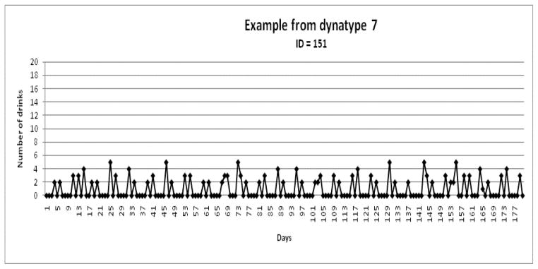
Dynatype 7 (N = 25): Set Point and Moderately Cyclic with Moderate Consumption
Figure 8.

Example from Dynatype 8 (N = 17): Set Point and Cyclic with High Consumption
External Validity
To demonstrate external validity of the eight dynatypes of alcohol users, a set of variables, not included in the cluster analysis but theoretically relevant to clustering variables, were used. A series of analysis of variance (ANOVA) were used to examine differences among dynatypes on continuous demographic and psychosocial variables, and logistic regression was used to examine differences on categorical demographic and psychosocial variables. Due to the non-normal distribution of frequency of drug use among participants who reported any drug use in the 6 month time period, generalized linear mixed model (GLIMM) with a negative binomial distribution was implemented. Significant differences among the eight dynatypes were found on gender, marital status, frequency of drug use, lifetime alcohol dependence, family history of alcohol use and SIP (see Table 4).
Table 4.
External validity of alcohol users typology
| Total sample | Dynatype 1 | Dynatype 2 | Dynatype 3 | Dynatype 4 | Dynatype 5 | Dynatype 6 | Dynatype 7 | Dynatype 8 | Test statistics | |
|---|---|---|---|---|---|---|---|---|---|---|
| Demographic characteristics | ||||||||||
| Age M (SD) | 39.57 (11.13) | 39.47 (10.22) | 43.05 (10.35) | 39.38 (10.65) | 39.60 (10.99) | 39.89 (12.91) | 42.07 (13.50) | 35.80 (10.99) | 38.94 (9.42) | F(7, 169) = 0.80 |
| Female N (%) | 109 (61.58) | 17 (89.47) | 6 (30.00) | 25 (64.10) | 6 (40.00) | 22 (78.57) | 8 (57.14) | 17 (68.00) | 8 (47.06) | χ2(7) = 20.25* |
| Married N (%)a | 34 (19.21) | 1 (5.26) | 0 | 12 (30.77) | 0 | 7 (25.00) | 5 (35.71) | 4 (16.00) | 5 (29.41) | χ2(7) = 18.43* |
| Hispanic N (%)a | 27 (15.25) | 4 (21.05) | 0 | 5 (12.82) | 1 (6.67) | 8 (28.57) | 2 (14.29) | 2 (8.00) | 5 (29.41) | χ2(7) = 12.63 |
| Race N (%) | ||||||||||
| White | 103 (58.19) | 11 (57.89) | 13 (65.00) | 21 (53.85) | 9 (60.00) | 15 (53.57) | 6 (42.86) | 18 (72.00) | 10 (58.82) | χ2(7) = 3.59 |
| Black | 39 (22.03) | 5 (26.32) | 6 (30.00) | 7 (17.95) | 1 (6.67) | 9 (32.14) | 6 (42.86) | 2 (8.00) | 3 (17.65) | |
| Other | 35 (19.77) | 3 (15.79) | 1 (5.00) | 11 (28.21) | 5 (33.33) | 4 (14.29) | 2 (14.29) | 5 (20.00) | 4 (23.53) | |
| Education Level N (%) | ||||||||||
| HS diploma or less | 91 (54.17) | 8 (44.44) | 11 (55.00) | 21 (60.00) | 8 (53.33) | 16 (59.26) | 10 (76.92) | 9 (39.13) | 8 (47.06) | χ2(7) = 6.29 |
| Some college or more | 77 (45.83) | 10 (55.56) | 9 (45.00) | 14 (40.00) | 7 (46.67) | 11 (40.74) | 3 (23.08) | 14 (60.87) | 9 (52.94) | |
| Employment N (%) | ||||||||||
| Full-time | 65 (36.72) | 8 (42.11) | 8 (40.00) | 14 (35.90) | 4 (26.67) | 8 (28.57) | 5 (35.71) | 10 (40.00) | 8 (47.06) | χ2(7) = 2.74 |
| Unemployed/Disabled/Retired | 71 (40.11) | 5 (26.32) | 8 (40.00) | 17 (43.59) | 9 (60.00) | 12 (42.86) | 7 (50.00) | 6 (24.00) | 7 (41.18) | |
| Other | 41 (23.16) | 6 (31.58) | 4 (20.00) | 8 (20.51) | 2 (13.33) | 8 (28.57) | 2 (14.29) | 9 (36.00) | 2 (11.76) | |
| Psychosocial Characteristics | ||||||||||
| Drug Users | ||||||||||
| N (%) | 81 (45.76) | 7 (36.84) | 10 (50.00) | 18 (46.15) | 8 (53.33) | 11 (39.29) | 9 (64.29) | 11 (44.00) | 7 (41.18) | χ2(7) = 3.58 |
| Number of Drug Use Daysb | ||||||||||
| M (SD) | 47.31 (60.81) | 31.00 (25.70) | 68.90 (71.07) | 40.11 (56.49) | 86.38 (73.48) | 50.09 (67.56) | 63.00 (75.72) | 11.64 (14.04) | 38.14 (63.67) | F(7, 73) = 2.36* |
| SCID N (%) | ||||||||||
| Personality disorder | 61 (34.46) | 10 (52.63) | 7 (35.00) | 9 (23.08) | 5 (33.33) | 9 (32.14) | 1 (7.14) | 12 (48.00) | 5 (29.41) | χ2(7) = 7.27 |
| Alcohol dependence (lifetime) | 88 (49.72) | 8 (42.11) | 13 (65.00) | 16 (41.03) | 11 (73.33) | 7 (25.00) | 9 (64.29) | 11 (44.00) | 13 (76.47) | χ2(7) = 18.49* |
| HAM | ||||||||||
| M (SD) | 19.53 (9.20) | 19.79 (9.65) | 21.20 (8.84) | 18.41 (10.39) | 21.27 (8.08) | 18.21 (9.85) | 22.36 (8.49) | 17.24 (7.66) | 21.53 (8.78) | F(7,169) = 0.86 |
| SIP | ||||||||||
| M (SD) | 5.44 (4.35) | 4.26 (4.09) | 5.05 (4.64) | 4.77 (4.00) | 9.47 (4.29) | 4.36 (3.87) | 5.71 (3.81) | 5.36 (3.91) | 6.82 (5.23) | F(7,169) = 2.89* |
| Father a Problem Drinker | ||||||||||
| N (%) | 57 (32.20) | 5 (26.32) | 5 (25.00) | 22 (56.41) | 5 (33.33) | 11 (39.29) | 3 (21.43) | 3 (12.00) | 3 (17.65 ) | χ2(7) = 78.23* |
| Treatment Services for Alcohol Use | ||||||||||
| N (%) | 48 (27.12) | 1 (5.26) | 4 (20.00) | 9 (23.08) | 7 (46.67) | 7 (25.00) | 8 (57.14) | 8 (32.00) | 4 (23.53) | χ2(7) = 12.74 |
| Readiness to Change N (%) | ||||||||||
| Precontemplation | 47 (26.55) | 6 (31.58) | 5 (25.00) | 13 (33.33) | 1 (6.67) | 12 (42.86) | 2 (14.29) | 5 (20.00) | 3 (17.65) | |
| Contemplation | 66 (37.29) | 4 (21.05) | 9 (45.00) | 14 (35.90) | 7 (46.67) | 5 (17.86) | 5 (35.71) | 12 (48.00) | 10 (58.82) | χ2(7) = 5.35 |
| Action | 64 (36.16) | 9 (47.37) | 6 (30.00) | 12 (30.77) | 7 (46.67) | 11 (39.29) | 7 (50.00) | 8 (32.00) | 4 (23.53) | |
p < .05
Fisher’s exact test
Based on participant who reported drug use
Discussion
The overarching goal of this study was to develop a typology of alcohol users. We integrated two advanced statistical methods, time series analysis and cluster analysis, each uniquely suited to understanding alcohol use behavior patterns over time. Examination of longitudinal daily and cyclic patterns of alcohol use based on individual trajectories and their application to group level data provided a new insight into the drinking behavior and its relation to commonly used measures of quantity and frequency of alcohol consumption and other indicators of alcohol use severity. We believe that the findings provide a scientifically meaningful typology of alcohol users that should be further examined in research and clinical settings.
Time series analysis
Time series provides a unique set of statistics, the autocorrelations, compared to nomothetic methods. In previous examples in the health sciences, the autocorrelation parameters have tended to be positive, restricted to the first-order term, and relatively consistent across subjects (Velicer, et al., 1992; Hoeppner, et al., 2008; Dierker et al., 2008). However, the pattern was more complex for our examples. There was a significant variability within the autocorrelation patterns among the 177 individuals. The first order autocorrelations observed in our sample of alcohol users ranged from −.76 to .72, and seventh order autocorrelations ranged from −.27 to .79.
The Set Point model was the most common, represented by a first order autocorrelation close to zero. This characterized five of the eight Dynatypes (Dynatypes 1, 2, 3, 7, &8). This suggests that alcohol is largely controlled by the current environment rather previous consumption behavior. Three of the Dynatypes involved low to moderate consumption patterns, perhaps what would be expected for this model. However, two Dynatypes involved high rates of consumption (Dynatypes 2 and 8).
Two of the Dynatypes involved a Fixed Effect Model (5 & 6), characterized by a positive autocorrelation indicating that current consumption is influenced by consumption on the previous day. One of these was a moderate consumption group, and the other was a high consumption group.
One Dynatype (4) was characterized by a Multiple Regulation Model. This model has a negative first order autocorrelation indicating that consumption levels will be opposite of the previous day.
The weekly cyclic pattern also occurred for four of the eight dynatypes (Dynatypes 1, 2, 7, and 8). All dynatypes with a cyclic pattern also were best described by a Set Point Model. This suggests that for these groups alcohol is largely under environmental or external control, both on a daily and weekly basis.
These findings confirm that alcohol use behavior is multidimensional, based on daily as well as cyclical (weekly) trends, with positive as well as negative autocorrelation patterns. Such high variability within the patterns of alcohol use is indicative of different models for alcohol regulation (Velicer, et al., 1992; Hoeppner, et al., 2008). Different patterns of drinking based on daily and weekly cycles suggest that biological as well as environmental and social components may play an important role in the pattern of alcohol use.
The slopes for each of the series were either not significant or significant but very small. The low variability in the estimated slope of the series indicates that alcohol use behavior is relatively stable over extended periods of time, which confirms Mundt’s et al. (1995) findings.
Study Sample
The study employed data from a sample of hazardous drinkers with MDD. There is a well-established association between hazardous drinking and MDD. In a key study examining a large community sample, Rodgers and colleagues (2000) found that hazardous drinkers were 1.89–2.34 times more likely to exceed clinical cutoffs on measures of depressive symptoms when compared to non-hazardous drinkers. In addition, a meta-analysis of 10 general population studies reported that heavy drinkers were consistently more likely to be depressed than light drinkers (Fillmore et al., 1998). Prospective studies have demonstrated that MDD and depressive symptoms are predictive of later hazardous drinking (e.g., Aalto-Setala, Marttunen, Tuulio-Henriksson, Poikolainen, & Lonnqvist, 2002; Wang and Patten,2001) and that hazardous drinking is predictive of later MDD (e.g., Brook, Brook, Zhang, Cohen, & Whiteman, 2002; Ross, Rehm, & Walsh, 1997). Furthermore, there is some evidence that hazardous drinking is associated with inferior depression treatment outcomes. For example, Worthington and colleagues (1996) found that heavier baseline alcohol consumption was significantly related to poorer response to fluoxetine in a sample of depressed outpatients who did not abuse substances. In addition, alcohol use has been found to play a major role in mortality among depressed patients (Moustgaard et al., 2013).
External Characteristics of the Eight Types
Dynatype 4(Multiple Regulation with High Consumption) appears to be the lowest functioning and the most at risk group. They report the highest level of alcohol use, with a heavy alcohol use episode followed by a day of relatively lower alcohol consumption. This group also has a high prevalence of lifetime alcohol dependence, the highest level of drug use, and the highest number of alcohol related problems. This group also appears to be the lowest socially functioning group, with none of the subjects reporting being married and less than 30% reporting full-time employment. On a positive note, this group reports the highest readiness to change their drinking, with over 90% of subjects characterized by this profile in the Contemplation or the Action stage.
On the basis of quantity and frequency of alcohol use, the most similar to Dynatype 4 are Dynatype 2 (Set Point and Highly Cyclical with High Consumption) and Dynatype 8 (Set Point and Cyclical with High Consumption). All three groups report high prevalence of lifetime alcohol dependence. There are interesting differences in daily and cyclical patterns of drinking behavior among these three groups. Both Dynatype 2 and 8 express a strong to moderate weekly cyclic pattern of drinking, whereas Dynatype 4 expresses a strong daily pattern, which may reflect an attempt to control their alcohol use by reducing their drinking after a day of heavy drinking episode. The other two groups appear to incorporate their alcohol consumption around an external social component.
Four groups, Dynatype 1, Dynatype 3, Dynatype 5, and Dynatype 7, reported similar frequency and quantity of alcohol use but different drinking behavior patterns. Profiles that express weekly cycles are less likely to be married than other profiles. While it seems that low frequency of alcohol use is closely related to lower severity of alcohol related problems relative to other profiles, more than 40% of the individuals characterized by these profiles reported lifetime alcohol dependence and a fourth of them utilized treatment services for alcohol use.
Dynatype 5 and Dynatype 6 present an interesting contrast. Both profiles present similar patterns of first and seventh autoregressive terms, but Dynatype 6 reports more than double the alcohol consumption of Dynatype 5. There are other differences between these two groups that are directly related to levels of alcohol use, such as increased frequency of lifetime alcohol dependence and utilization of alcohol treatment services among individuals characterized by Dynatype 6. However, subjects characterized by Dynatype 5 have a higher rate of personality disorders and are more likely to have a father with a history of alcohol abuse.
Dynatype 3 had a very low level of alcohol use but report having a father with history of alcohol abuse. We can speculate that having a close family member who had history of alcohol abuse may be a protective factor, such that individuals drink less as a preventive measure against alcohol abuse. This hypothesis is in opposition to well established genetic models of developing substance abuse disorders. Perhaps there is a non-linear relationship between genetic history and substance abuse.
Implications of the Typology of Alcohol Users
The results of this study have important implications for the research and clinical area of addictive behaviors. To date, most studies on alcohol use have been based on unrefined and insensitive measures of alcohol consumption, which can distort the conclusions drawn from such studies. The common methodological approach among longitudinal studies is based on a limited number of time points and, with the data averaged across groups, provide highly generalizable results but no information on actual drinking behavior of any of the study participants. However, a combination of nomothetic and idiographic methodology, can potentially advance our understanding of alcohol use behaviors.
Identification of the eight subgroups of alcohol users has the potential to further advance the understanding of the substance use behavior and consequently improve treatment outcomes. We have shown that temporal patterns of drinking behavior are as important in defining subtypes of alcohol users as are quantity and frequency of alcohol use. Our findings demonstrate that individuals with very similar quantities of alcohol consumption can have different temporal patterns of drinking behavior. These daily and cyclic patterns of alcohol use may be an important behavioral correlate affecting the severity of consequences associated with drinking and may provide insight into the processes involved in the development of alcohol abuse and dependence.
High heterogeneity within patterns of drinking can have strong clinical implications. It appears that daily patterns of drinking play a different role in the drinking behavior than weekly cycles, such that a strong daily negative pattern may be related to an attempt at controlling level of substance use whereas weekly cycles are related to social and lifestyle activities.
Tailoring treatment to specific behavior patterns that these eight dynatypes manifest could improve the clinical outcomes and consequently allocate available resources in a more effective fashion. We were able to show that the population of alcohol users is highly heterogeneous and that a one-size–fits-all approach may be highly ineffective in research as well as in clinical settings.
Limitations
This study has several limitations. First, cluster analysis is an exploratory method that serves more to develop hypotheses rather than to test them. Therefore, it should not be used solely as an outcome variable but more as a tool for further exploration of highly heterogeneous populations. This analytical approach requires replication of the findings for more extensive generalization of the results. Second, this study is based on a limited sample of ambulatory patients whose primary diagnosis was Major Depressive Disorder and who were recruited into the original randomized trial. Replication of the findings in a more general population of alcohol users is necessary to confirm the results. Third, this study is based on a secondary data analysis, and it was not powered to allow for multiple group comparison. Therefore, external validity could be compromised by insufficient power to detect all significant psychosocial and demographic differences among the eight profiles of alcohol users. Fourth, the predictive validity of the identified dynatypes through longitudinal research is necessary to better understand how individuals characterized by different patterns of alcohol use respond to treatment and their long term prognoses. Fifth, the results rely on the primary measure employed, Alcohol Timeline Followback. The measure involves recall assisted by a calendar. While widely employed with good validity information, the measure is subject to all the problems associated with recall measures. Having alcohol consumption assessed concurrently by a method such as telemetric monitoring (Goodwin, Velicer, & Intille, 2008) should produce a more accurate assessment.
Conclusions
Through the innovative combination of idiographic and nomothetic methodology, we identified eight distinct profiles of alcohol users, based on their daily and weekly patterns of alcohol use as well as longitudinal trajectories of drinking. We demonstrated that this population of substance users is highly heterogeneous, and commonly used measures of quantity and frequency of alcohol use are not sensitive enough to accurately reflect the complexity of their drinking behavior. The existence of these subtypes has implication for both the analysis of alcohol treatment data and the design of treatments. The use of a Hierarchical Linear Model with Dynatype as a factor nested within intervention condition is potentially the optimal design. The examination of the external validity confirmed the theoretical relevance of different patterns of alcohol use and their different associations with psychosocial and demographic characteristics related to substance use. These findings show that integration of time series analysis and cluster analysis is an effective methodological approach to advance our understanding of the unique patterns of heterogeneity in a sample of alcohol users.
Highlights.
Idiographic methodology examined the longitudinal patterns of alcohol use.
A dynamic cluster analysis was employed to identify homogenous longitudinal patterns.
The analysis employed 180 daily observations of alcohol use for a sample of 177.
Eight distinct patterns of alcohol users were identified.
The patterns may be used to design tailored interventions for problem drinkers.
Acknowledgments
This paper was partially supported Grant DA020112 from NIDA (Velicer, PI) and Grant AA013895 from NIAAA (Ramsey, PI).
Footnotes
Publisher's Disclaimer: This is a PDF file of an unedited manuscript that has been accepted for publication. As a service to our customers we are providing this early version of the manuscript. The manuscript will undergo copyediting, typesetting, and review of the resulting proof before it is published in its final citable form. Please note that during the production process errors may be discovered which could affect the content, and all legal disclaimers that apply to the journal pertain.
Contributor Information
Magdalena Harrington, Cancer Prevention Research Center, University of Rhode Island.
Wayne F. Velicer, Cancer Prevention Research Center, University of Rhode Island
Susan Ramsey, The Warren Alpert Medical School of Brown University and Rhode Island Hospital.
References
- Aalto-Setala T, Marttunen M, Tuulio-Henriksson A, Poikolainen K, Lonnqvist J. Depressive symptoms in adolescence as predictors of early adulthood depressive disorders and maladjustment. American Journal of Psychiatry. 2002;159:1235–1237. doi: 10.1176/appi.ajp.159.7.1235. [DOI] [PubMed] [Google Scholar]
- Aldenderfer MS, Blashfield RK. Cluster Analysis. Beverly Hills, CA: Sage Publications; 1984. [Google Scholar]
- Aloia MS, Goodwin MS, Velicer WF, Arnedt JT, Zimmerman M, Skrekas J, Harris S, Millman RP. Time Series Analysis of Treatment Adherence Patterns in Individuals with Obstructive Sleep Apnea. Annuals of Behavioral Medicine. 2008;36:44–53. doi: 10.1007/s12160-008-9052-9. [DOI] [PubMed] [Google Scholar]
- Babbin SF, Velicer WF, Aloia M, Kushida C, Berry R. Time series analysis of adherence to treatment for obstructive sleep apnea. Annuals of Behavioral Medicine. 2011;41:S170. (Abstract) [Google Scholar]
- Babor TF, Hofmann M, DelBoca FK, Hesselbrock V, Meyer RE, Dolinsky ZS, et al. Types of alcoholics, I. Evidence for an empirically derived typology based on indicators of vulnerability and severity. Archives of General Psychiatry. 1992;49:599–608. doi: 10.1001/archpsyc.1992.01820080007002. [DOI] [PubMed] [Google Scholar]
- Basu D, Ball SA, Feinn R, Gelernter J, Kranzler HR. Typologies of drug dependence: Comparative validity of a multivariate and four univariate models. Drug and Alcohol Dependence. 2004;73:289–300. doi: 10.1016/j.drugalcdep.2003.11.004. [DOI] [PubMed] [Google Scholar]
- Brewer RD, Swahn MH. Binge drinking and violence. Journal of American Medical Association. 2005;294:616–618. doi: 10.1001/jama.294.5.616. [DOI] [PubMed] [Google Scholar]
- Brook DW, Brook JS, Zhang C, Cohen P, Whiteman M. Drug use and the risk of major depressive disorder, alcohol dependence, and substance use disorders. Archives of General Psychiatry. 2002;59:1039–1044. doi: 10.1001/archpsyc.59.11.1039. [DOI] [PubMed] [Google Scholar]
- Cronbach LJ, Gleser GC. Assessing similarity between profiles. Psychological Bulletin. 1953;50:456–473. doi: 10.1037/h0057173. [DOI] [PubMed] [Google Scholar]
- Del Boca FK, Darkes J, Greenbaum PE, Goldman MS. Up close and personal: Temporal variability in the drinking of individual college students during their first year. Journal of Consulting and Clinical Psychology. 2004;72:155–164. doi: 10.1037/0022-006X.72.2.155. [DOI] [PubMed] [Google Scholar]
- Dierker L, Stolar M, Lloyd-Richardson E, Tiffany S, Flay B, Collins L, et al. Tobacco, alcohol, and marijuana use among first-year U.S. college students: A time series analysis. Substance Use & Misuse. 2008;43:680–699. doi: 10.1080/10826080701202684. [DOI] [PMC free article] [PubMed] [Google Scholar]
- Fillmore KM, Golding JM, Graves KL, Kniep S, Leino EV, Romelsjo A, Shoemaker C, Ager CR, Allebeck P, Ferrer HP. Alcohol consumption and mortality I. Characteristics of drinking groups. Addiction. 1998;93:183–203. doi: 10.1046/j.1360-0443.1998.9321834.x. [DOI] [PubMed] [Google Scholar]
- First MB, Spitzer RL, Gibbon M, Williams JBW. Structured Clinical Interview for DSM-IV Axis I Disorders-Patient Edition. New York: New York State Psychiatric Institute; 1997. [Google Scholar]
- Glass GV, Willson VL, Gottman JM. Design and analysis of time series experiments. Charlotte, NC: Information Age Publishing; 2008. [Google Scholar]
- Goldman MS, Greenbaum PE, Darkes J, Obremski-Brandon K, Del Boca FK. How many versus how much: 52 weeks of alcohol consumption in emerging adults. Psychology of Addictive Behaviors. 2011;25:16–27. doi: 10.1037/a0021744. [DOI] [PMC free article] [PubMed] [Google Scholar]
- Goodwin MS, Velicer WF, Intille SS. Telemetric monitoring in the behavior sciences. Behavior Research Methods. 2008;40:328–341. doi: 10.3758/brm.40.1.328. [DOI] [PubMed] [Google Scholar]
- Hoeppner BB, Goodwin MS, Velicer WF, Mooney ME, Hatsukami DK. Detecting longitudinal patterns of daily smoking following drastic cigarette reduction. Addictive Behaviors. 2008;33:623–639. doi: 10.1016/j.addbeh.2007.11.005. [DOI] [PMC free article] [PubMed] [Google Scholar]
- Hoeppner BB, Barnett NP, Jackson KM, Colby SM, Kahler CW, Monti PM, Read J, Tevyaw T, Wood M, Corriveau D, Fingeret A. Daily College Student Drinking Patterns across the First Year of College. Journal of Studies on Alcohol and Drugs. 2012;73:613–624. doi: 10.15288/jsad.2012.73.613. [DOI] [PMC free article] [PubMed] [Google Scholar]
- Humphreys K, Rosenheck R. Sequential validation of cluster analytic subtypes of homeless veterans. American Journal of Community Psychology. 1995;23:75–98. [Google Scholar]
- Jarvik ME. Further observations on nicotine as the reinforcing agent in smoking. In: Dunn WL Jr, editor. Smoking Behavior: Motives and incentives. Washington, D. C: V. H. Winston; 1973. [Google Scholar]
- Leventhal H, Cleary PD. The smoking problem: A review of the research and theory in behavioral risk modification. Psychological Bulletin. 1980;88:370–405. doi: 10.1037/0033-2909.88.2.370. [DOI] [PubMed] [Google Scholar]
- Maibach EW, Maxfield A, Ladin K, Slater M. Translating health psychology into effective health communication: The American health styles audience segmentation project. Journal of Health Psychology. 1996;1:261–277. doi: 10.1177/135910539600100302. [DOI] [PubMed] [Google Scholar]
- Marczinski CA, Combs SW, Fillmore MT. Increased sensitivity to the disinhibiting effects of alcohol in binge drinkers. Psychology of Addictive Behaviors. 2007;21:346–354. doi: 10.1037/0893-164X.21.3.346. [DOI] [PubMed] [Google Scholar]
- McLellan AT, Alterman AI, Cacciola J, Metzger D, O’Brien CP. A new measure of substance abuse treatment: Initial studies of the Treatment Services Review. Journal of Nervous and Mental Disease. 1992;180:101–110. doi: 10.1097/00005053-199202000-00007. [DOI] [PubMed] [Google Scholar]
- Milligan GW. An examination of the effect of six types of error perturbation of fifteen clustering algorithms. Psychometrica. 1980;45:325–342. [Google Scholar]
- Milligan GW, Cooper MC. An examination of procedures determining the number of clusters in a data set. Psychometrica. 1985;50:159–179. [Google Scholar]
- Milligan GW, Cooper MC. Methodology review: Clustering methods. Applied Psychological Measurement. 1987;11:329–354. [Google Scholar]
- Miller IW, Bishop S, Norman WH, Maddever H. The Modified Hamilton Rating Scale for Depression: Reliability and validity. Psychiatry Research. 1985;14:131–142. doi: 10.1016/0165-1781(85)90057-5. [DOI] [PubMed] [Google Scholar]
- Miller WR, Tonigan JS, Longabaugh R. The Drinker Inventory of Consequences (DrInC): An Instrument for assessing adverse consequences of alcohol abuse. 4. US Department of Health and Human Services, Public Health Service, National Institute of Health, National Institute on Alcohol Abuse and Alcoholism; Rockville, MD: 1995. (Project MATCH Monograph Series) (NIH Publication No. 95-3911) [Google Scholar]
- Molenaar PCM. A manifesto on psychology as idiographic science: Bringing the person back into the scientific psychology, this time forever. Measurement. 2004;2:201–218. [Google Scholar]
- Molenaar PCM, Campbell CG. The new person – specific paradigm in psychology. Current Direction in Psychological Science. 2009;18:112–117. [Google Scholar]
- Moss HB, Chen CM, Yi HY. Subtypes of alcohol dependence in a nationally representative sample. Drug and Alcohol Dependence. 2007;91:149–158. doi: 10.1016/j.drugalcdep.2007.05.016. [DOI] [PMC free article] [PubMed] [Google Scholar]
- Moustgaard H, Joutseeniemi K, Sihvo S, Martikainen P. Alcohol-related deaths and social factors in depression mortality: A register-based follow-up of depressed in-patients and antidepressant users in Finland. Journal of Affective Disorders. 2013;148:278–285. doi: 10.1016/j.jad.2012.12.008. [DOI] [PubMed] [Google Scholar]
- Mundt JC, Searles JS, Perrine MW, Helzer JE. Cycles of alcohol dependence: Frequency-domain analyses of daily drinking logs for matched alcohol-dependent and nondependent subjects. Journal of Studies on Alcohol. 1995;56:491–499. doi: 10.15288/jsa.1995.56.491. [DOI] [PubMed] [Google Scholar]
- Norman GJ, Velicer WF. Developing an empirical typology for regular exercise. Preventive Medicine. 2003;37:635–645. doi: 10.1016/j.ypmed.2003.09.011. [DOI] [PubMed] [Google Scholar]
- Norman GJ, Velicer WF, Fava JL, Prochaska JO. Dynamic typology clustering within the stages of change for smoking cessation. Addictive Behaviors. 1998;23:139–153. doi: 10.1016/s0306-4603(97)00039-7. [DOI] [PubMed] [Google Scholar]
- Quinlan KP, Brewer RD, Siegel P, Sleet DA, Mokdad AH, Shults RA, et al. Alcohol impaired driving among U.S. adults, 1993–2002. American Journal of Preventative Medicine. 2005;28:346–350. doi: 10.1016/j.amepre.2005.01.006. [DOI] [PubMed] [Google Scholar]
- Rapkin BD, Luke DA. Cluster analysis in community research: Epistemology and practice. American Journal of Community Psychology. 1993;21:247–277. [Google Scholar]
- Rodgers B, Korten AE, Jorm AF, Jacomb PA, Christensen H, Henderson AS. Non-linear relationships in associations of depression and anxiety with alcohol use. Psychological Medicine. 2000;30:421–432. doi: 10.1017/s0033291799001865. [DOI] [PubMed] [Google Scholar]
- Rollnick S, Heather N, Gold R, Hall W. Development of a short ‘readiness to change’ questionnaire for use in brief, opportunistic interventions among excessive drinkers. British Journal of Addiction. 1992;87:743–754. doi: 10.1111/j.1360-0443.1992.tb02720.x. [DOI] [PubMed] [Google Scholar]
- Ross H, Rehm J, Walsh G. Patterns of alcohol consumption and psychiatric disorders among Ontario adults. Contemporary Drug Problems. 1997;24:533–556. [Google Scholar]
- Russell MA. Nicotine chewing gum as a substitute for smoking. British Medical Journal. 1977;1:1060–1063. doi: 10.1136/bmj.1.6068.1060. [DOI] [PMC free article] [PubMed] [Google Scholar]
- Schachter S. Nicotine regulation in heavy and light smokers. Journal of Experimental Psychology: General. 1977;106:5–12. [Google Scholar]
- Shaw SY, Shah L, Jolly AM, Wylie JL. Identifying heterogeneity among injection drug users: A cluster analysis approach. American Journal of Public Health. 2008;98:1430–1437. doi: 10.2105/AJPH.2007.120741. [DOI] [PMC free article] [PubMed] [Google Scholar]
- Sobell LC, Sobell MB. Alcohol Timeline Followback (TLFB) Users’ Manual. Toronto, Canada: Addiction Research Foundation; 1996. [Google Scholar]
- Solomon RL. The opponent-process theory of acquired motivation. American Psychologist. 1980;35:691–712. doi: 10.1037//0003-066x.35.8.691. [DOI] [PubMed] [Google Scholar]
- Solomon RL, Corbit JD. An opponent-process theory of motivation: II. Cigarette addiction. Journal of Abnormal Psychology. 1973;81:158–171. doi: 10.1037/h0034534. [DOI] [PubMed] [Google Scholar]
- Solomon RL, Corbit JD. An opponent-process theory of motivation: I. Temporal dynamics of affect. Psychological Review. 1974;81:119–145. doi: 10.1037/h0036128. [DOI] [PubMed] [Google Scholar]
- Standerwick K, Davies C, Tucker L, Sheron N. Binge drinking, sexual behavior and sexually transmitted infection in the UK. International Journal of STD & AIDS. 2007;18:810–813. doi: 10.1258/095646207782717027. [DOI] [PubMed] [Google Scholar]
- Substance Abuse and Mental Health Services Administration. NSDUH Series H-36, HHS Publication No. SMA 09-4434. Office of Applied Studies; Rockville, MD: 2009. Results from the 2008 National Survey on Drug Use and Health: National findings. [Google Scholar]
- Velicer WF. Applying Idiographic Research Methods: Two Examples. In: Reading C, editor. Data and context in statistics education: Towards an evidence-based society; Proceedings of the Eighth International Conference on Teaching Statistics (ICOTS8, July, 2010); Ljubljana, Slovenia. Voorburg, The Netherlands: International Statistical Institute; 2010. www.stat.auckland.ac.nz/~iase/publications.php. [Google Scholar]
- Velicer WF, Harrop J. The reliability and accuracy of time series model identification. Evaluation Review. 1983;7:551–560. [Google Scholar]
- Velicer WF, Hughes SL, Fava JL, Prochaska JO, DiClemente CC. An empirical typology of subjects within stage of change. Addictive Behaviors. 1995;20:299–320. doi: 10.1016/0306-4603(94)00069-b. [DOI] [PubMed] [Google Scholar]
- Velicer WF, McDonald RP. Time series analysis without model identification. Multivariate Behavioral Research. 1984;19:33–47. doi: 10.1207/s15327906mbr1901_2. [DOI] [PubMed] [Google Scholar]
- Velicer WF, Redding CA, Anatchkova MD, Fava JL, Prochaska JO. Identifying cluster subtypes for the prevention of adolescent smoking acquisition. Addictive Behaviors. 2007;32:228–247. doi: 10.1016/j.addbeh.2006.03.041. [DOI] [PubMed] [Google Scholar]
- Velicer WF, Redding CA, Richmond RL, Greeley J, Swift W. A time series investigation of three nicotine regulation models. Addictive Behaviors. 1992;17:325–345. doi: 10.1016/0306-4603(92)90039-x. [DOI] [PubMed] [Google Scholar]
- Velicer WF, Rossi JS. A dynamic typology and cross sequential profiles: An example. Paper presented at the Psychometric Society Meeting; Toronto, Canada. 1986. [Google Scholar]
- Velicer WF, Molenaar P. Time Series Analysis. In: Schinka J, Velicer WF, editors. Research Methods in Psychology. 2. 2013. Volume 2 of Handbook of Psychology. [Google Scholar]
- Velicer WF, Babbin SF, Palumbo R. Idiographic Applications in Behavioral Medicine: Issues of Ergodicity and Generalizability. In: Molenaar PM, Lerner, Newell, editors. Handbook of Developmental Systems Theory and Methodology. New York: Guilford Publications; pp. 00–00. (in press) [Google Scholar]
- Velicer WF, Palumbo R, Babbin SF. Time Series Analysis. In: Cautin RL, Lilienfeld SO, editors. Encyclopedia of Clinical Psychology. Hoboken, NJ: Wiley-Blackwell; pp. 00–00. (in press) [Google Scholar]
- Vogel-Sprott M, Chipperfield B, Hart DM. Family history of problem drinking among young male social drinkers: Reliability of the Family Tree Questionnaire. Drug and Alcohol Dependence. 1985;16:251–256. doi: 10.1016/0376-8716(85)90049-3. [DOI] [PubMed] [Google Scholar]
- Wang JL, Patten SB. A prospective study of sex-specific effects of major depression on alcohol consumption. Canadian Journal of Psychiatry. 2001;46:422–425. doi: 10.1177/070674370104600507. [DOI] [PubMed] [Google Scholar]
- Worthington J, Fava M, Agustin C, Alpert J, Nierenberg AA, Pava JA, Rosenbaum JF. Consumption of alcohol, nicotine, and caffeine among depressed outpatients. Psychosomatics. 1996;37:518–522. doi: 10.1016/S0033-3182(96)71515-3. [DOI] [PubMed] [Google Scholar]