Circadian clocks optimally adapt to sunlight for reliable synchronization

Abstract

Circadian oscillation provides selection advantages through synchronization to the daylight cycle. However, a reliable clock must be designed through two conflicting properties: entrainability to synchronize internal time with periodic stimuli such as sunlight, and regularity to oscillate with a precise period. These two aspects do not easily coexist, because better entrainability favours higher sensitivity which may sacrifice regularity. To investigate conditions for satisfying the two properties, we analytically calculated the optimal phase–response curve with a variational method. Our results indicate an existence of a dead zone, i.e. a time period during which input stimuli neither advance nor delay the clock. A dead zone appears only when input stimuli obey the time course of actual solar radiation, but a simple sine curve cannot yield a dead zone. Our calculation demonstrates that every circadian clock with a dead zone is optimally adapted to the daylight cycle.

1. Introduction

Circadian oscillators are prevalent in organisms from bacteria to humans and serve to synchronize bodies with the environmental 24 h cycle [1,2]. Although the molecular implementation of oscillation is species-specific [3–6], every circadian clocks satisfies two requirements to achieve reliable synchronization to the environment: entrainability to synchronize internal time with periodic stimuli and regularity to oscillate with a precise period. Circadian clocks are acquired through evolution independently in bacteria, fungi, plants and animals [7]. Nonetheless, entrainability and regularity constitute major characteristics conserved in all circadian clocks [6], which strongly suggest that these two properties are essential for survival. A main source of interference with regularity is discreteness of molecular species, i.e. molecular noise [8–13]. Many studies have analysed the resistance mechanisms of circadian oscillators against noise [14–17]. Regarding entrainability, circadian clocks synchronize their internal time with the environmental cycle via sunlight, and its effect depends on the wavelength or fluence, as well as on the phase of the stimulation. However, entrainability and regularity are conflicting factors, because circadian clocks with better entrainability are sensitive not only to the periodic light stimuli, but also to the molecular noise which interferes with regularity.

Because both regularity and entrainability are important adaptive values, we expect actual circadian oscillators to optimally satisfy these two factors (figure 1). Here, we investigate the optimal phase–response curve (PRC), which is both entrainable and regular, in the phase oscillator model [18] by using the Euler–Lagrange variational method. Our main finding is the inherent existence of a dead zone in the PRC: optimality is achieved only when the PRCs have a time period during which light stimuli neither advance nor delay the clock (figure 2a). In other words, a PRC with a dead zone (figure 2a) is better adapted than those without a dead zone (figure 2b). This result is intriguing, because a dead zone, with which oscillators tend to be unaffected by stimuli (i.e. lower entrainability), achieves better entrainability. We also tested this with two types of input stimuli: a solar radiation-type input that simulated the time course of solar radiation intensity (cf. equation (2.24) and figure 4a) and a simple sinusoidal input (sine curve). Surprisingly, the dead zone in the optimal PRC emerges only for the solar radiation-type input, not for the sinusoidal input. Many experimental studies reported the existence of a dead zone in various species (figure 2c,d show experimentally observed PRCs of fruitfly [19] and mouse [20], respectively). Our results indicate that circadian oscillators in various species have adapted to solar radiation for reliable synchronization.

Figure 1.

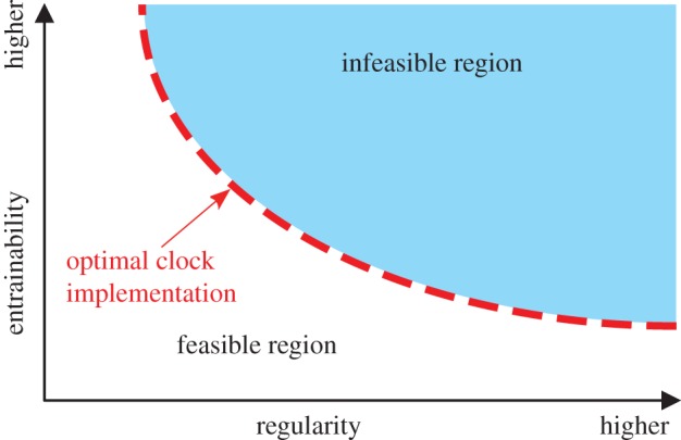
Illustrative relation between two trade-off properties: entrainability and regularity. There is an infeasible region with respect to entrainability and regularity (coloured area), inside which no clocks can be implemented. Actual circadian clocks are considered to optimally satisfy them and such optimal clocks lie on the edge between feasible and infeasible regions (thick-dashed line).

Figure 2.

Illustrations of typical PRCs (a) with and (b) without a dead zone. Experimentally observed PRCs as a function of time in (c) fruitfly (Drosophila) [19] and (d) mouse (Mus) [20] with light pulses (circles) and their trigonometric fitting curves (solid line). Shaded and non-shaded regions indicate subjective night and day, respectively.

Figure 4.

(a) Solar radiation input of equation (2.24), where the shaded region denotes night. (b) Comparison between solar radiation input (equation (2.24)) and actual observed irradiance data taken from Vick & Moss [39]. The solar radiation input (solid line) and the observed data (circle) refer to left and right axes, respectively. (c) Gene regulatory circuit of hypothetical circadian clock. In this example, x₁ and x₂ describe mRNA and protein, respectively, and x₃ represses the transcription of x₁. Light stimulus increases the translational efficiency. (d) Time course of x_LC,k(ϕ) (equation (3.2)), which is a variable to be multiplied by the parameter ρ (equation (3.1)).

2. Models and methods

2.1. Phase oscillator model

Circadian oscillators basically comprise interaction between mRNAs and proteins, whose dynamics can be modelled by differential equations. A circadian oscillator of N molecular species can be represented by

2.1

where the N-dimensional vector x = (x₁, x₂, … ,x_N) denotes the concentration of molecular species (mRNAs or proteins). The effect of noise on genetic oscillators has been a subject of considerable interest, and noise-resistant mechanisms have been extensively studied [14–17,21–23]. In general, the dynamics of the ith molecular concentration in a circadian oscillator subjected to molecular noise is described by the following Langevin equation (Stratonovich interpretation):

2.2

where Q_i(x) is an arbitrary function representing the multiplicative terms of the noise, ξ_i(t) is white Gaussian noise with the correlation 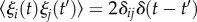(a bracket denotes expectation), and ρ is a model parameter.

Circadian oscillators synchronize to environmental cycles by responding to a periodic input signal (light stimuli). We let ρ in equation (2.2) be stimulated by the input signal: for example, ρ can be the degradation rate (for the sake of simplicity, we consider that the input signal affects only one parameter). We use equation (2.2) for calculating regularity and entrainability of circadian oscillators.

2.2. Definition of regularity

Because the circadian oscillator of equation (2.2) is subjected to noise, its period varies cycle to cycle. We use the term regularity for the period variance of the oscillation (higher regularity corresponds to smaller period variance). Let us first consider the case without input signals (i.e. ρ is constant). As equation (2.1) exhibits periodic oscillation, we can naturally define the phase ϕ ∈ [0,2π) on equation (2.1) by

2.3

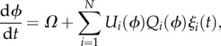
where Ω = 2π/T is the angular frequency of the oscillation (T is a period of the oscillation). The phase ϕ in equation (2.3) is defined only on a closed orbit of the unperturbed limit-cycle oscillation. However, we can expand the definition into the entire x = (x₁, x₂, … ,x_N) space, where the equiphase surface is referred to as the isochron ℐ(ϕ) (figure 3a). By using standard stochastic phase reduction [18], equation (2.2) can be transformed into the following Langevin equation with respect to the phase variable ϕ (Stratonovich interpretation):

2.4

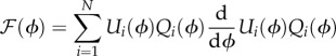
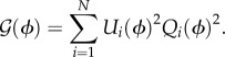
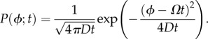
where U(ϕ) = (U₁(ϕ), … ,U_N(ϕ)) is an infinitesimal PRC (iPRC) 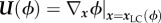, and we abbreviated Q_i(x_LC(ϕ)) as Q_i(ϕ). iPRC U_i(ϕ) quantifies the extent of phase advance or delay when perturbed along an x_i coordinate direction at phase ϕ. The N-dimensional vector x_LC(ϕ) denotes a point on the limit-cycle trajectory at phase ϕ, where LC stands for limit cycle. The value of iPRC U_i(ϕ) is calculated as a solution of an adjoint equation [24] or as the set of eigenvectors of a monodromy matrix in the Floquet theory [18] for arbitrary oscillators. Let P(ϕ; t) be the probability density function of ϕ at time t. From equation (2.4), the Fokker–Planck equation (FPE) [25] of P(ϕ; t) is given by

2.5

where

2.6

and

2.7

Introducing a slow variable φ = ϕ – Ωt, the FPE of the probability density function Π(φ; t) = P(ϕ = φ + Ωt; t) is given by

2.8

Figure 3.

(a) Illustration of the isochron ℐ(ϕ), the solid and dashed lines describing a limit-cycle trajectory and its isochron drawn at intervals of π/6, respectively. (b) Relation between the phase variance and the period variance in Langevin equation (2.2) (the solid lines represent trajectories of the Langevin equation). is the variance of the phase ϕ at time t = T and is the variance of the first passage time from 0 to 2π, which can be approximated by 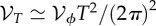. (d) Arnold tongue (coloured region), which shows the parameter region for synchronization to an input signal, with respect to the signal angular frequency ω (vertical axis) and the signal strength χ (horizontal axis). The dashed line is a linear approximation (equation (2.17)) of the border of the Arnold tongue when the input strength χ is sufficiently small.

With sufficiently weak noise, Π(φ; t) is a slowly fluctuating function of t. In such cases, ℱ(φ + Ωt) and 𝒢(φ + Ωt) fluctuate much faster than Π(φ; t), thus these two terms can be averaged for one period while keeping Π(φ; t) constant (phase averaging). In other words, we separate time scales between ℱ(φ + Ωt), 𝒢(φ + Ωt) and Π(φ; t). By phase averaging, ℱ(φ + Ωt) vanishes because of the periodicity (use integration by parts), yielding

2.9

with

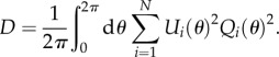2.10

See Kuramoto [18] for further details of stochastic phase reduction and the phase-averaging procedure. From equation (2.9), because Π(φ = ϕ–Ωt; t)[ = P(ϕ; t)] obeys a simple one-dimensional diffusion equation, its solution is represented by

2.11

Equation (2.11) shows that the variance of the phase after one period T is

In equation (2.4), the average period corresponds to the mean first passage time with ϕ starting from 0 to 2π, and the period variance is the variance of the first passage time. Because direct calculation of the period variance is difficult, we approximate the period variance with the phase variance , after Kori et al. [26]. As the phase ϕ crosses a threshold ϕ = 2π with gradient 2π/T without noise, there is a scaling relation 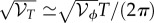for sufficiently weak noise [26] (figure 3b). Consequently, the variance of the period is approximated by

2.12

2.3. Definition of entrainability

The entrainment property is an important characteristic of limit-cycle oscillators and attracts attention in systems biology [27–32]. For instance, a period mismatch in coupled oscillators is known to enhance entrainability in genetic oscillators [31]. Light stimuli affect the rate constants, i.e. the parameter ρ in equation (2.2) is perturbed as ρ + dρ by the input signal. Phase dynamics of equation (2.2) can be viewed as representing that of a tilted periodic potential (i.e. ratchet) subjected to noise. Because a synchronizable condition corresponds to the existence of stable points in the ratchet-like potential, the entrainability can be discussed without considering the noise. Consequently, in contrast to the calculation of regularity, in the evaluation of the entrainability, we consider a case without molecular noise (i.e. Q_i(x) = 0 in equation (2.2)).

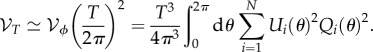
Let p(ωt) be an input signal with angular frequency ω. Considering a weak periodic input signal dρ = χp(ωt), where χ is the signal strength (χ ≥ 0), and applying the phase reduction approach to equation (2.2), the time evolution of the phase variable ϕ is given by

2.13

with F_i(ϕ; ρ) = F_i(x_LC(ϕ); ρ) and

2.14

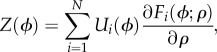
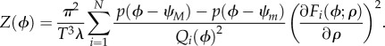
where Z(ϕ) is the PRC with respect to the parameter ρ and corresponds to experimentally observed PRCs. In order to distinguish Z(ϕ) from iPRC U_i(ϕ), we will refer to Z(ϕ) as the parametric PRC (pPRC) [33]. Note that the definition of measured PRCs is different from pPRCs Z(ϕ) in a rigorous definition; the experimentally measured PRCs quantify the phase shift Δϕ caused by light stimuli, whereas pPRCs Z(ϕ) are normalized by the strength of perturbation, i.e. . Therefore, the ranges of the measured pPRCs have limitation −π ≤ Δϕ < π, whereas pPRCs Z(ϕ) do not. The phase reduction can yield reliable results only when the perturbed trajectory is close to the unperturbed limit-cycle trajectory (i.e. χ is sufficiently small).

We next evaluate the extent of synchronization to the periodic input signal. By introducing another slow variable ψ = ϕ–ωt in equation (2.13), we can again apply the phase-averaging procedure, which yields

2.15

with ΔΩ = Ω – ω and

2.16

The oscillator of interest can synchronize to input signals when there is a stable solution of ψ in (equation (2.15)). The stable solution is an intersection point of Θ(ψ) and –ΔΩ with dΘ/dψ < 0 (an empty circle in figure 3c). Then, a condition for the existence of a stable solution is

2.17

where and .

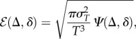
We define entrainability, the extent of synchronization to the periodic input signal, by the width of the Arnold tongue, which is a domain with respect to χ (signal strength) and ω (signal angular frequency). The shaded region in figure 3d represents the Arnold tongue; with parameters χ and ω inside the Arnold tongue, the oscillator can synchronize to a periodic input signal. Because equation (2.17) constitutes a linear approximation of the Arnold tongue for sufficiently small χ, the width of the Arnold tongue is given by χ(Θ(ψ_M) – Θ(ψ_m)) under the linear approximation. Thus, we define the entrainability ℰ, or the extent of synchronization, as

2.18

Intuitively, a circadian oscillator with better entrainability (i.e. larger ℰ) can synchronize to an input signal that has a period further from that of the oscillator. The calculation above is standard in the phase reduction approach, and further details are available in Kuramoto [18].

2.4. Variational method

We use the variational method to calculate the optimal PRCs which maximize the entrainability ℰ subject to constant variance (the optimal solutions correspond to the edge in figure 1, which is described by the thick-dashed line). The constrained optimization of U_i(ϕ) can be intuitively interpreted as maximization of weighted area (equation (2.18)), where the input being the weight, with constant area under the squared magnitude (equation (2.12)). In simple terms, the optimality is reached when the magnitude of the PRC is small during intervals when the input magnitude is small (and vice versa). In the context of neuronal oscillators, a study [34] has used the variational method to calculate the optimal PRCs for stochastic synchrony (noise-induced synchronization [35,36]).

The variational equation to be optimized is

2.19

where λ is the Lagrange multiplier. Note that variational equation (2.19) is similar to Harada et al. [37], which optimizes the input signal for the maximal entrainment under constant power of the input. The variational condition δℒ[U] = 0 yields the optimal iPRC

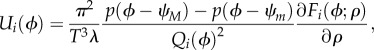2.20

and the pPRC is calculated with equation (2.14):

2.21

Because ψ_M and ψ_m themselves depend on U_i(ϕ), they have to satisfy a self-consistent condition, i.e. equation (2.18) is maximal with ψ_M and ψ_m. Consequently, we maximize the following function:

2.22

with

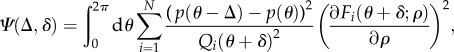2.23

where Δ = ψ_M – ψ_m and δ = ψ_m. The optimal iPRC can be obtained by first finding the maximum solution of Ψ(Δ, δ) with respect to Δ and δ, and then substituting the obtained solution ψ_m = δ and ψ_M = δ + Δ into equations (2.20) and (2.21).

2.5. Input signal of solar radiation model

Optimal PRCs depend on input signals, as seen in equations (2.20) and (2.21). The most common synchronizer in circadian oscillators is sunlight, for which the strength is determined by 24 h-periodic solar irradiance. The solar irradiance is calculated by I = I₀ cos ϑ and I = 0 when the sun is above the horizon (0 ≤ ϑ < π) and below the horizon (π ≤ ϑ < 2π), respectively, where ϑ is the zenith angle and I₀ is the maximum irradiance [38]. It can be approximated by

2.24

where ramp(x) is the ramp function defined by ramp(x) = x for x ≥ 0 and ramp(x) = 0 for x < 0. We call equation (2.24) the solar radiation input, whose plot is shown in figure 4a (the shaded region represents night). In order to show the validity of the solar radiation modelling, we compare equation (2.24) with observed irradiance data from Vick & Moss [39], which are shown in a dual axis plot of figure 4b. In figure 4b, equation (2.24) is plotted by the solid line (left axis) and the observed data by the dashed line (right axis). The solar radiation input of equation (2.24) is shifted horizontally, so that equation (2.24) becomes a good fit to the data. From figure 4b, the solar radiation input is in good agreement with the observed data, which verifies the validity of equation (2.24) as a solar radiation model.

For comparison, we also use a sinusoidal input, which is common in nonlinear sciences:

2.25

Note that p(ωt) = B + sin(ωt), where B is an arbitrary constant, also yields the same optimal PRCs as equation (2.25), because a constant B in the signal is offset in equations (2.20)–(2.23). Although a constant B does not play any roles in formation of the optimal PRCs, different B result in different Arnold tongues in general. For calculating the optimal PRCs, we use equations (2.24) and (2.25).

3. Results

3.1. Optimal phase–response curve of solar radiation input

Light stimuli generally affect the oscillatory dynamics multiplicatively, i.e. they act on the rate constants or transcriptional efficiency of the gene regulatory circuits [3,40]. We assume that the jth molecular species includes a parameter ρ as

3.1

where represents the terms that do not include ρ, and x_k is the concentration of the kth molecular species. Here, k∈{1,2, … ,N} can take any value, regardless of j (both j ≠ k and j = k are allowed). For example, let figure 4c be a gene regulatory circuit of a hypothetical circadian clock, where symbols → and ⊣ represent positive and negative regulations and x_i are molecular species (see Novák & Tyson [41] for typical motifs of biochemical oscillators). Suppose x₁ and x₂ are mRNA and corresponding protein, respectively, and light stimuli increase the translational efficiency. In this case, the dynamics of light entrainment can be described by equation (3.1) with j = 2, k = 1 and ρ being the translation rate. In equation (3.1), although we can also consider an alternative case 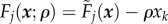(a negative sign), the optimal pPRCs remain unchanged under the inversion which is seen from equations (2.21) and (2.23). Consequently, we consider only the positive case to calculate the optimal PRCs (i.e. equation (3.1)). However, note that relations between iPRCs and pPRCs are affected by the inversion of the sign, and the difference matters when considering biological feasibility.

When using phase reduction, the dynamics of the limit cycle are considered on the unperturbed limit-cycle trajectories x_LC, and hence the points on the limit cycle can be uniquely determined by the phase ϕ. Consequently, under the phase reduction, x_k is replaced by x_LC,k(ϕ) in equation (3.1), where x_LC,k(ϕ) is the kth coordinate of x_LC (i.e. in equation (2.20)). Here, corresponds to the time course of the concentration of the kth molecular species. Because x_LC,k(ϕ) constitutes a core clock component and is generally a smooth 2π-periodic function, we approximate it with a sinusoidal function:

3.2

where u is the initial phase and α denotes the amplitude of the oscillation (figure 4d). To ensure , we set 0 ≤ α ≤ 1, and α = 0 recovers the additive case. Because the initial phase u does not play any role (u is offset by δ in equation (2.23)) when the white Gaussian noise is additive (i.e. Q_i(x) ∝ 1), we also set u = 0. The parametric approximation of equation (3.2) enables an almost closed form for the overall calculations. Although we assumed in equation (3.1) that effects of ρ only depend on x_k, we can generalize equation (3.1) to , where K(x) is a nonlinear function and is assumed to be well approximated by 1 – αsin(ϕ + u). By this generalization, our theory can be applied to other possible light entrainment mechanisms such as the intercellular coupling [42]. Our model needs only details about molecular species which have light input entry points but not about a whole molecular network. However, this advantage, in turn, means that we cannot specify iPRCs U_i(ϕ) of molecular species not having light input entry points. Consequently, for a noise term Q_i(x), we assume that the white Gaussian noise is additive and is present only in the jth coordinate equation (, where q is the noise intensity and Q_i(ϕ) = 0 for i ≠ j).

Figure 5a–c shows the landscape of Ψ(Δ,δ) as functions of Δ and δ, and figure 5d–f expresses the optimal iPRCs U_j(ϕ) and pPRCs Z(ϕ) for the solar radiation input (an explicit expression of Ψ(Δ, δ) is given in appendix A). The optimal PRC shape does not depend on the model parameters such as the period T, its variance , or noise intensity q. These three parameters only act on the magnitude of the PRCs (i.e. the vertical scaling of the PRCs). Consequently, we normalized T = 1, , and q = 1, as shown in figure 5. As the optimal PRCs depend on α, Ψ(Δ, δ) is plotted for three cases: α = 0, (figure 5a), α = 0.5 (figure 5b) and α = 1.0 (figure 5c), where the maximal points (Δ, δ) yield the optimal PRCs using equations (2.20) and (2.21). The maximal parameters Δ and δ are calculated numerically. Figure 5d–f describes the optimal iPRCs (solid line) and pPRCs (dashed line) for α = 0, 0.5 and 1.0, respectively. When α = 0, i.e. the input signal is additive, Ψ(Δ,δ) achieves a maximum for Δ = π and arbitrary δ, yielding sinusoidal PRCs as the optimal solution (figure 5d). Although the input signal p(ϕ) is not sinusoidal, the optimal PRCs obtained using the variational method become sinusoidal. In other words, considering optimality, resonator-type oscillators have an advantage over integrator-type oscillators. For α > 0, the input signal p(ϕ) depends on the concentration of the kth molecular species. From figure 5b, the optimal parameters for α = 0.5 are (Δ, δ) = (2.31, 1.99) and (3.98, 4.30), which are different from Δ = π (these two sets yield symmetric PRCs with respect to the horizontal axis). Figure 5e shows the optimal iPRCs U_j(ϕ) and pPRCs Z(ϕ) for α = 0.5. Interestingly, the optimal iPRCs and pPRCs for α = 0.5 have a dead zone (region of in figure 5e) in which the input signal neither advances nor delays the clock. From equations (2.20)–(2.21) and the solar radiation input of equation (2.24), the optimal PRCs inevitably include a dead zone if the optimal Δ is not π. For α = 1.0, there are four sets of parameters (Δ, δ) that give optimal PRCs: (2.30, 2.72), (2.30, 1.26), (3.98, 3.56) and (3.98, 5.02) (PRCs with these four sets are symmetric with each other with respect to the horizontal axis or ϕ = 3π/2). Consequently, the optimal PRCs shown in figure 5f have a dead zone as in the case of α = 0.5.

Figure 5.

(a–c) Landscape of Ψ(Δ, δ) as a function of Δ and δ with solar radiation input (equation (2.24)) for (a) α = 0, (b) α = 0.5 and (c) α = 1.0, where the maximum points are parameters for the optimal PRC. (d–f) Optimal PRCs with solar radiation input: (d) α = 0, (e) α = 0.5 and (f) α = 1.0. In (d–f), the solid and dashed lines denote iPRCs U_j(ϕ) and pPRCs Z(ϕ), respectively (in (d), solid and dashed lines are indistinguishable). The maximal parameters (Δ,δ) for (d–f) are (d) (π, 0), (e) (2.31, 1.99) and (f) (2.30, 2.72). In (d), a parallel shift of the PRC is also optimal (δ can be an arbitrary value). In (e), symmetric PRCs with respect to the horizontal axis are also optimal. In (f), symmetric PRCs with respect to the horizontal axis or ϕ = 3π/2 are also optimal (see the text). The pPRCs correspond to experimentally observed PRCs.

3.2. Dead zone length

From the results discussed above, the optimal PRCs have a dead zone when α > 0. We next studied the length of the dead zone as a function of α (figure 6a) and improvements in the entrainability induced by the dead zone (figure 6b) for the solar radiation input. Because the dead zone, which is a null interval in PRCs, emerges when the optimal parameter is Δ ≠ π, we can naturally define its length as

3.3

where Δ is the maximum value of Ψ(Δ, δ). As seen in figure 6a, a dead zone clearly exists when α > 0, and the length increases with increasing α for α < 0.8. Even for α = 0.1, when the oscillation amplitude of x_LC,k(ϕ) (the concentration of a molecular species modulated by the light-sensitive parameter ρ; cf. figure 4d) is very small, we observe a dead zone with a length of L = 0.475, which corresponds to about 3 h within 24 h, indicating the universality of having a dead zone in order to attain optimality. The improvement in the entrainability that is induced by a dead zone is calculated by comparing the entrainability of the optimal PRCs with that of typical sinusoidal PRCs. We consider sinusoidal functions for both the iPRC U_j(ϕ) and pPRC Z(ϕ) by setting

3.4

and

3.5

where c is the parameter to be optimized so that entrainability is maximized for each α (see appendix B for the explicit expressions). Equations (3.4) and (3.5) are scaled, so that they satisfy the constraints on the period variance (equation (2.12)). We calculated the ratios

3.6

where and represent the entrainabilities for the cases of the sinusoidal iPRC and pPRC, respectively, calculated for the solar radiation input. For the sinusoidal iPRC of equation (3.4), the entrainability is calculated with pPRC via equation (2.14). R_U and R_Z quantify the improvement rate of the optimal PRCs over the sinusoidal iPRC (R_U) and pPRC (R_Z). In figure 6b, the solid and dashed lines show R_U and R_Z, respectively, as a function of α. Both ratios monotonically increase as α increases, which shows that the optimal PRC with a dead zone exhibits better entrainability when the oscillation of x_LC,k(ϕ) has a larger amplitude. When the concentration of x_LC,k(ϕ) is low, the effects of the input signal on the circadian oscillators are smaller. This is because pPRC Z(ϕ), which quantifies the extent of the phase shift owing to the stimulation of the parameter, depends on the concentration x_LC,k(ϕ) (see equation (2.14)). However, even within the range ϕ where x_LC,k(ϕ) has smaller values, the iPRC U_j(ϕ) contributes to an increase in the variance of the period, regardless of the concentration. From this, we see that having an iPRC with a smaller magnitude when the concentration of x_LC,k(ϕ) is smaller results in a smaller variance, which results in a larger entrainability for a constant variance of the period. Although this qualitatively explains the benefit of a dead zone, for some input values, the optimal PRCs may not contain a dead zone for any value of α. This will be shown in the following.

Figure 6.

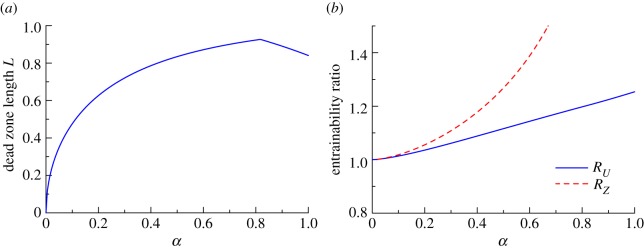
(a) α-Dependence of the dead zone length L. (b) α-Dependence of the entrainability ratios R_U (solid line) and R_Z (dashed line; equation (3.6)). R_U and R_Z are the ratios of the entrainability of the optimal PRC to that of the sinusoidal iPRC (equation (3.4)) and the pPRC (equation (3.5)), respectively.

3.3. Optimal phase–response curve of sinusoidal input

Because the optimal PRCs depend on input signals (equations (2.20) and (2.21)), we next consider a typical periodic input signal, a sinusoidal function (equation (2.25)). In this case, Ψ(Δ, δ) is calculated in a closed form (an explicit expression of Ψ(Δ, δ) is given in appendix A), which is plotted as functions of Δ and δ in figure 7a–c for three cases: α = 0 (figure 7a), α = 0.5 (figure 7b) and α = 1.0 (figure 7c). As can been seen from figure 7a–c, Ψ(Δ, δ) yields the maximal value for (Δ, δ) = (π, nπ) for 0 < α ≤ 1, where n is an integer and when α = 0, δ can take any value. Figure 7d–f expresses the optimal iPRCs U_j(ϕ) and pPRCs Z(ϕ) for the sinusoidal input. For α = 0, the optimal PRC is sinusoidal (figure 7d) and for α = 0.5, the optimal PRC is still close to a sinusoidal function (figure 7e). When increasing α to α = 1.0, the PRC diverges from the sinusoidal function and exhibits almost positive values (figure 7f). We see that the optimal PRCs owing to equations (2.20) and (2.21) do not exhibit a dead zone for any α-values (figure 7d–f) when the input signal is a simple sinusoidal function.

Figure 7.

(a–c) Landscape of Ψ(Δ, δ) as functions of Δ and δ with sinusoidal input for (a) α = 0, (b) α = 0.5 and (c) α = 1.0, where the maximum points are parameters for the optimal PRC. (d–f) Optimal PRCs with sinusoidal input (equation (2.25)): (d) α = 0, (e) α = 0.5 and (f) α = 1.0, where the solid and dashed lines denote iPRCs U_j(ϕ) and pPRCs Z(ϕ). The maximal parameter (Δ, δ) is (π, 0) in all cases. In (d), a parallel shift of the PRC is also optimal (δ can be an arbitrary value). PRCs that are symmetric with respect to the horizontal axis are also optimal. The pPRCs correspond to experimentally observed PRCs.

4. Discussion

The existence of a dead zone optimizes both entrainability and regularity. It is rather obvious that optimization of regularity alone leads to a dead zone [43], because null response means no effect by any kind of fluctuations. Our result instead shows that optimality of both entrainability and regularity, which are in a trade-off relationship, is uniquely achieved by a dead zone. Our finding is fairly general, because a dead zone always exists in an optimal PRC unless α = 0 (additive stimulation). Along with the fact that T, σ_T and q affect only the scaling of the optimal PRCs, when the input signal affects the dynamics multiplicatively (i.e. α > 0), the existence of a dead zone always provides a synchronization advantage. This is supported by many experimental studies of various species that report the existence of a dead zone in the PRC [1] (cf. figure 2c,d). Our general result suggests that circadian oscillators have fully adapted to solar radiation to improve synchronization. Indeed, many experimental findings imply that circadian oscillators have adapted to actual solar radiation [44]: for various animals, light–dark (LD) cycles that include a twilight period result in better entrainability than do abrupt LD cycles (on–off protocols) [44]. In this regard, another interesting problem is optimal entrainment [37] of circadian clocks by light stimuli. As two different input signals, the solar radiation and sinusoidal inputs, yield the same optimal PRCs for α = 0, optimal inputs and optimal PRCs do not have one-to-one correspondence. Thus, the optimal inputs are not trivial and this problem should be pursued in our future studies.

The solar radiation input plays an essential role, because it yields a dead zone in the optimal PRC, whereas a sinusoidal signal does not (figure 7). In other words, oscillators that are entrained by stimuli other than solar radiation may not exhibit a dead zone in their PRCs. This is indeed found in mammals. Mammals possess a master clock in their suprachiasmatic nucleus (SCN), which receives light stimuli via retinal photoreceptors, and peripheral clocks in body cells [45]. The peripheral oscillators are entrained by several stimuli such as feeding and signals from the SCN through chemical pathways (e.g. hormones) [45,46]. By injection experiments of a hormone, Balsalobre et al. [47] reported that the PRCs of the peripheral oscillators in the liver do not have a dead zone.

Our result also agrees with other experimental observations. Our theory implies that a dead zone should be located where the concentration x_LC,k(ϕ) is low (0 ≤ ϕ ≤ π in figure 4d), and that to achieve optimality, the concentration of x_LC,k(ϕ) should be maximal in the region where the PRCs exhibit a large phase shift. In Drosophila, the timeless (tim) gene is regarded as the molecular implementation of x_LC,k(ϕ). It is experimentally known that light enhances the degradation of the gene product (the TIM protein) [48,49], and the TIM protein peaks during the late evening. Figure 2c shows observations of the PRC of Drosophila against light pulses as a function time from Hall & Rosbash [19]; circles describe the experimental data, and the solid line expresses a trigonometric curve fitting (fourth order). Because the centre of the part of the PRC that can be phase shifted approximately corresponds to the peak of the concentration, as denoted above, when estimated from the PRC alone, the concentration peak of the TIM protein should occur at about 18 h. This time is also close to the experimental evidence (i.e. late evening). Therefore, our theory can be used to hypothesize further molecular behaviour affected by light stimuli.

In summary, we have constructed a model that regards circadian oscillators as a global optimization of entrainability and regularity. We have shown that our model is consistent with much experimental evidence as mentioned above. The extension and improvement of our method are possible and they are left as an area of future study.

Appendix A. Explicit expression of Ψ(Δ, δ)

A.1. Solar radiation input case

For the solar radiation input case (equation (2.24)), Ψ(Δ, δ) is given by

A1

with

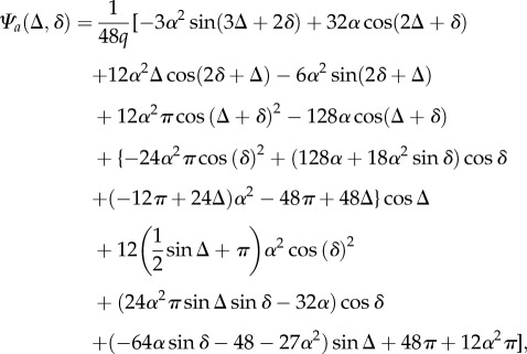where . We show equation (A 1) as functions of Δ and δ in figure 5d–f.

A.2. Sinusoidal input case

For the sinusoidal input case (equation (2.25)), Ψ(Δ, δ) is given by

A2

We plot equation (A 2) as functions of Δ and δ in figure 7d–f.

Appendix B. Explicit expression of sinusoidal phase–response curves

B.1. Sinusoidal infinitesimal phase–response curve

An explicit expression for the sinusoidal iPRC (equation (3.4)) is

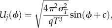B1

which yields the period variance of . Then, the corresponding pPRC is given by

B2

where we used equation (2.14).

B.2. Sinusoidal parametric phase–response curve

For the pPRC Z(ϕ) to be a sinusoidal function, the iPRC U_j(ϕ) must be

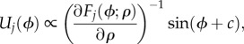B3

where we used equation (2.14). An explicit expression of equation (B 3) is

B4

where 𝒩(c) is a normalizing term

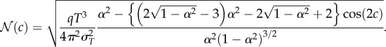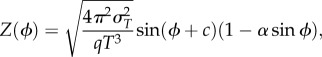
Equation (B 4) is normalized, so that the period variance becomes . Using equation (2.14), the corresponding pPRC is a sinusoidal function:

B5

which is an explicit expression of the sinusoidal pPRC (equation (3.5)).

Funding statement

This work was supported by the Global COE programme ‘Deciphering Biosphere from Genome Big Bang’ from MEXT, Japan (Y.H. and M.A.); grant-in-aid for Young Scientists B (no. 25870171) from MEXT, Japan (Y.H.); grant-in-aid for Scientific Research on Innovative Areas ‘Biosynthetic machinery’ from MEXT, Japan (M.A.).

References

- 1.Refinetti R. 2005. Circadian physiology, 2nd edn Boca Raton, FL: Taylor & Francis. [Google Scholar]
- 2.Gonze D. 2011. Modeling circadian clocks: roles, advantages, and limitations. Cent. Eur. J. Biol. 6, 712–729. ( 10.2478/s11535-011-0062-4) [DOI] [Google Scholar]
- 3.Johnsson A, Engelmann W. 2007. The biological clock and its resetting by light. In Photobiology: the science of life and light (ed. L Olof Björn), pp. 321–388 New York, NY: Springer. [Google Scholar]
- 4.Hubbard KE, Robertson FC, Dalchau N, Webb AAR. 2009. Systems analyses of circadian networks. Mol. Biosyst. 5, 1502–1511. ( 10.1039/b907714f) [DOI] [PubMed] [Google Scholar]
- 5.Ukai H, Ueda HR. 2010. Systems biology of mammalian circadian clocks. Annu. Rev. Physiol. 72, 579–603. ( 10.1146/annurev-physiol-073109-130051) [DOI] [PubMed] [Google Scholar]
- 6.Johnson CH, Stewart PL, Egli M. 2011. The cyanobacterial circadian system: from biophysics to bioevolution. Annu. Rev. Biophys. 40, 143–167. ( 10.1146/annurev-biophys-042910-155317) [DOI] [PMC free article] [PubMed] [Google Scholar]
- 7.Young MW, Kay SA. 2001. Time zones: a comparative genetics of circadian clocks. Nat. Rev. Genet. 2, 702–715. ( 10.1038/35088576) [DOI] [PubMed] [Google Scholar]
- 8.Kærn M, Elston TC, Blake WJ, Collins JJ. 2005. Stochasticity in gene expression: from theories to phenotypes. Nat. Rev. Genet. 6, 451–464. ( 10.1038/nrg1615) [DOI] [PubMed] [Google Scholar]
- 9.Perkins TJ, Swain PS. 2009. Strategies for cellular decision-making. Mol. Syst. Biol. 5, 326 ( 10.1038/msb.2009.83) [DOI] [PMC free article] [PubMed] [Google Scholar]
- 10.Raser JM, O'Shea EK. 2005. Noise in gene expression: origins, consequences, and control. Science 309, 2010–2013. ( 10.1126/science.1105891) [DOI] [PMC free article] [PubMed] [Google Scholar]
- 11.Eldar A, Elowitz MB. 2010. Functional roles for noise in genetic circuits. Nature 467, 167–173. ( 10.1038/nature09326) [DOI] [PMC free article] [PubMed] [Google Scholar]
- 12.Hasegawa Y, Arita M. 2012. Fluctuating noise drives Brownian transport. J. R. Soc. Interface 9, 3554–3563. ( 10.1098/rsif.2012.0603) [DOI] [PMC free article] [PubMed] [Google Scholar]
- 13.Viney M, Reece SE. 2013. Adaptive noise. Proc. R. Soc. B 280, 20131104 ( 10.1098/rspb.2013.1104) [DOI] [PMC free article] [PubMed] [Google Scholar]
- 14.Gonze D, Halloy J, Goldbeter A. 2002. Robustness of circadian rhythms with respect to molecular noise. Proc. Natl Acad. Sci. USA 99, 673–678. ( 10.1073/pnas.022628299) [DOI] [PMC free article] [PubMed] [Google Scholar]
- 15.Forger DB, Peskin CS. 2005. Stochastic simulation of the mammalian circadian clock. Proc. Natl Acad. Sci. USA 102, 321–324. ( 10.1073/pnas.0408465102) [DOI] [PMC free article] [PubMed] [Google Scholar]
- 16.Morelli LG, Jülicher F. 2007. Precision of genetic oscillators and clocks. Phys. Rev. Lett. 98, 228101 ( 10.1103/PhysRevLett.98.228101) [DOI] [PubMed] [Google Scholar]
- 17.Rougemont J, Naef F. 2007. Dynamical signatures of cellular fluctuations and oscillator stability in peripheral circadian clocks. Mol. Syst. Biol. 3, 93 ( 10.1038/msb4100130) [DOI] [PMC free article] [PubMed] [Google Scholar]
- 18.Kuramoto Y. 2003. Chemical oscillations, waves, and turbulence. Mineola, NY: Dover Publications. [Google Scholar]
- 19.Hall JC, Rosbash M. 1987. Genes and biological rhythms. Trends Genet. 3, 185–191. ( 10.1016/0168-9525(87)90231-9) [DOI] [Google Scholar]
- 20.Daan S, Pittendrigh CS. 1976. A functional analysis of circadian pacemakers in noctornal rodents II. The variability of phase response curves. J. Comp. Physiol. 106, 253–266. ( 10.1007/BF01417857) [DOI] [Google Scholar]
- 21.Vilar JMG, Kueh HY, Barkai N, Leibler S. 2002. Mechanisms of noise-resistance in genetic oscillators. Proc. Natl Acad. Sci. USA 99, 5988–5992. ( 10.1073/pnas.092133899) [DOI] [PMC free article] [PubMed] [Google Scholar]
- 22.Scott M, Ingalls B, Kærn M. 2006. Estimations of intrinsic and extrinsic noise in models of nonlinear genetic networks. Chaos 16, 026107 ( 10.1063/1.2211787) [DOI] [PubMed] [Google Scholar]
- 23.Yoda M, Ushikubo T, Inoue W, Sasai M. 2007. Roles of noise in single and coupled multiple genetic oscillators. J. Chem. Phys. 126, 115101 ( 10.1063/1.2539037) [DOI] [PubMed] [Google Scholar]
- 24.Izhikevich EM. 2007. Dynamical systems in neuroscience: the geometry of excitability and bursting. Cambridge, MA: MIT Press. [Google Scholar]
- 25.Risken H. 1989. The Fokker–Planck equation: methods of solution and applications, 2nd edn Berlin, Germany: Springer. [Google Scholar]
- 26.Kori H, Kawamura Y, Masuda N. 2012. Structure of cell networks critically determines oscillation regularity. J. Theor. Biol. 297, 61–72. ( 10.1016/j.jtbi.2011.12.007) [DOI] [PubMed] [Google Scholar]
- 27.Gonze D, Goldbeter A. 2000. Entrainment versus chaos in a model for a circadian oscillator driven by light–dark cycles. J. Stat. Phys. 101, 649–663. ( 10.1023/A:1026410121183) [DOI] [Google Scholar]
- 28.Hasty J, Dolnik M, Rottschäfer V, Collins JJ. 2002. Synthetic gene network for entraining and amplifying cellular oscillations. Phys. Rev. Lett. 88, 148101 ( 10.1103/PhysRevLett.88.148101) [DOI] [PubMed] [Google Scholar]
- 29.Bagheri N, Taylor SR, Meeker K, Petzold LR, Doyle FJ., III 2008. Synchrony and entrainment properties of robust circadian oscillators. J. R. Soc. Interface 5, S17–S28. ( 10.1098/rsif.2008.0045.focus) [DOI] [PMC free article] [PubMed] [Google Scholar]
- 30.Abraham U, Granada AE, Westermark PO, Heine M, Kramer A, Herzel H. 2010. Coupling governs entrainment range of circadian clocks. Mol. Syst. Biol. 6, 438 ( 10.1038/msb.2010.92) [DOI] [PMC free article] [PubMed] [Google Scholar]
- 31.Hasegawa Y, Arita M. 2013. Enhanced entrainability of genetic oscillators by period mismatch. J. R. Soc. Interface 10, 20121020 ( 10.1098/rsif.2012.1020) [DOI] [PMC free article] [PubMed] [Google Scholar]
- 32.Erzberger A, Hampp G, Granada AE, Albrecht U, Herzel H. 2013. Genetic redundancy strengthens the circadian clock leading to a narrow entrainment range. J. R. Soc. Interface 10, 20130221 ( 10.1098/rsif.2013.0221) [DOI] [PMC free article] [PubMed] [Google Scholar]
- 33.Taylor SR, Gunawan R, Petzold LR, Doyle FJ., III 2008. Sensitivity measures for oscillating systems: application to mammalian circadian gene network. IEEE Trans. Automat. Control 53, 177–188. ( 10.1109/TAC.2007.911364) [DOI] [PMC free article] [PubMed] [Google Scholar]
- 34.Abouzeid A, Ermentrout B. 2009. Type-II phase resetting curve is optimal for stochastic synchrony. Phys. Rev. E 80, 011911 ( 10.1103/PhysRevE.80.011911) [DOI] [PubMed] [Google Scholar]
- 35.Teramae J, Tanaka D. 2004. Robustness of the noise-induced phase synchronization in a general class of limit cycle oscillators. Phys. Rev. Lett. 93, 204103 ( 10.1103/physrevlett.93.204103) [DOI] [PubMed] [Google Scholar]
- 36.Nakao H, Arai K, Kawamura Y. 2007. Noise-induced synchronization and clustering in ensembles of uncoupled limit-cycle oscillators. Phys. Rev. Lett. 98, 184101 ( 10.1103/PhysRevLett.98.184101) [DOI] [PubMed] [Google Scholar]
- 37.Harada T, Tanaka H-A, Hankins MJ, Kiss IZ. 2010. Optimal waveform for the entrainment of a weakly forced oscillator. Phys. Rev. Lett. 105, 088301 ( 10.1103/physrevlett.105.088301) [DOI] [PubMed] [Google Scholar]
- 38.Hartmann DL. 1994. Global physical climatology. San Diego, CA: Academic Press. [Google Scholar]
- 39.Vick BD, Moss TA. 2013. Adding concentrated solar power plants to wind farms to achieve a good utility electrical load match. Solar Energy 92, 298–312. ( 10.1016/j.solener.2013.03.007) [DOI] [Google Scholar]
- 40.Golombek DA, Rosenstein RE. 2010. Physiology of circadian entrainment. Physiol. Rev. 90, 1063–1102. ( 10.1152/physrev.00009.2009) [DOI] [PubMed] [Google Scholar]
- 41.Novák B, Tyson JJ. 2008. Design principles of biochemical oscillators. Nat. Rev. Mol. Cell Biol. 9, 981–991. ( 10.1038/nrm2530) [DOI] [PMC free article] [PubMed] [Google Scholar]
- 42.Ohta H, Yamazaki S, McMahon DG. 2005. Constant light desynchronizes mammalian clock neurons. Nat. Neurosci. 8, 267–269. ( 10.1038/nn1395) [DOI] [PubMed] [Google Scholar]
- 43.Pfeuty B, Thommen Q, Lefranc M. 2011. Robust entrainment of circadian oscillators requires specific phase response curves. Biophys. J. 100, 2557–2565. ( 10.1016/j.bpj.2011.04.043) [DOI] [PMC free article] [PubMed] [Google Scholar]
- 44.Fleissner G, Fleissner G. 2002. Perception of natural Zeitgeber signals. In Biological rhythms (ed. V Kumar), pp. 83–93 Berlin, Germany: Springer. [Google Scholar]
- 45.Dibner C, Schibler U, Albrecht U. 2010. The mammalian circadian timing system: organization and coordination of central and peripheral clocks. Annu. Rev. Physiol. 72, 517–549. ( 10.1146/annurev-physiol-021909-135821) [DOI] [PubMed] [Google Scholar]
- 46.Dickmeis T. 2009. Glucocorticoids and the circadian clock. J. Endocrinol. 200, 3–22. ( 10.1677/JOE-08-0415) [DOI] [PubMed] [Google Scholar]
- 47.Balsalobre A, Brown SA, Marcacci L, Tranche F, Kellendonk C, Reichardt HM, Schütz G, Schibler U. 2000. Resetting of circadian time in peripheral tissues by glucocorticoid signaling. Science 29, 2344–2347. ( 10.1126/science.289.5488.2344) [DOI] [PubMed] [Google Scholar]
- 48.Hardin PE. 2005. The circadian timekeeping system of Drosophila. Curr. Biol. 15, R714–R722. ( 10.1016/j.cub.2005.08.019) [DOI] [PubMed] [Google Scholar]
- 49.Xie Z, Kulasiri D. 2007. Modelling of circadian rhythms in Drosophila incorporating the interlocked PER/TIM and VRI/PDP1 feedback loops. J. Theor. Biol. 245, 290–304. ( 10.1016/j.jtbi.2006.10.028) [DOI] [PubMed] [Google Scholar]