The evolution of continuous learning of the structure of the environment

Abstract

Continuous, ‘always on’, learning of structure from a stream of data is studied mainly in the fields of machine learning or language acquisition, but its evolutionary roots may go back to the first organisms that were internally motivated to learn and represent their environment. Here, we study under what conditions such continuous learning (CL) may be more adaptive than simple reinforcement learning and examine how it could have evolved from the same basic associative elements. We use agent-based computer simulations to compare three learning strategies: simple reinforcement learning; reinforcement learning with chaining (RL-chain) and CL that applies the same associative mechanisms used by the other strategies, but also seeks statistical regularities in the relations among all items in the environment, regardless of the initial association with food. We show that a sufficiently structured environment favours the evolution of both RL-chain and CL and that CL outperforms the other strategies when food is relatively rare and the time for learning is limited. This advantage of internally motivated CL stems from its ability to capture statistical patterns in the environment even before they are associated with food, at which point they immediately become useful for planning.

1. Introduction

Effective control of behaviour on the part of an animal requires at least a minimal grasp of the structure of the ecological niche in which it is situated. For many species, the requisite knowledge can be quite sophisticated. Thus, a forager can benefit from a representation of the spatial layout of its range, a social animal—of the dominance hierarchy in its group, and a tool user—of the cascading effects of the various actions that the tools afford. While such representations are clearly beneficial when fully in place, their acquisition—both over evolutionary time and in individual learning—presents a problem: intermediate steps in the acquisition process may not be useful and in any case are not necessarily incrementally reinforced. In this paper, we examine such learning, in which a learner continuously attempts to learn all regularities in its environment regardless of their immediate value. We refer to this mode of learning as continuous, and focus on its relationship with reinforced learning in the context of a foraging task. We chose to refer to the learning mode of interest as ‘continuous’ because the alternative (‘unreinforced’) would be misleading in that occasional reinforcement does occur in the tasks that we explore.

In psychology, the intuition behind reinforced learning [1,2] is captured by Thorndike's [3] ‘Law of Effect’, which pertains to reinforcement learning as well as to associative learning, such as classical and operant conditioning. Most learning models studied by evolutionary biologists and behavioural economists in the vast fields of game theory and decision-making fall under this rubric [2,4,5]. However, animals (and especially humans) are likely to use a much richer representation of their environment than captured by simple ‘n-armed bandit’ models of reinforcement learning. A richer representation—a causal model or a cognitive map—can be constructed by reinforcement learning through backward chaining, where items associated with primary reinforcers can become secondary reinforcers, with which additional items can be associated in turn. This process can result in associative chains or networks of secondary reinforcers through which the learner can navigate to the primary reinforcer [6–8]. The drawback of using this process for constructing a world model is that it requires that each item in the chain be reinforced and turned into a secondary reinforcer before the next item down the road can be learned.

An alternative to backward chaining is learning the environment in a non-reinforced fashion. For example, instead of learning diagnostic features only in the vicinity of food, an animal may be internally motivated to acquire a stream of data along its path, from which it can construct a world model [9]. There is ample evidence for the existence of such learning in animals, ranging from studies of exploratory behaviour in mice and rats [10] to research on play behaviour in young animals [11–13] and in adult individuals [14–16]. Young animals, in particular, often show interest in novel objects, which they can distinguish from dozens of previously encountered objects without reinforcement [17]. There are also indications that explorative actions are not random, but directed at uncovering regularities that may be adaptive [18]. Animals may also be self-motivated to learn to recognize their social peers or group members and to acquire information about them [19]. Finally, seldom-reinforced or non-reinforced, continuous learning (CL) in the present sense may be involved in some of the most advanced forms of cognition, such as vocal learning and language acquisition [20–22], and its mechanisms are becoming a central theme of exploration in machine learning, psychology and neuroscience (reviewed in [23]).

While CL seems useful, it can also be very costly in terms of memory and computation. First, it requires focusing on relevant input while discarding unnecessary information. Second, the relevant input may take the form of a constant stream of data whose segmentation and statistical analysis can be taxing [24]. How could learning mechanisms capable of addressing these problems [20,25,26] have evolved in the first place?

In this paper, we study the conditions under which CL is more adaptive than reinforced learning in the context of animal foraging and examine how it could have evolved on top of the basic learning by association. We used agent-based computer simulations to compare three learning strategies: local reinforcement learning (LR) that associates environmental cues with food only if they are experienced in the same locality as the food; reinforcement learning with chaining (RL-chain), which supports construction of a world model through backward chaining; and CL, which uses not only the same associative mechanisms as the first two strategies, but also seeks statistical regularities in the relations among all items in the environment, regardless of initial association with food. To identify the ecological conditions that favour the evolution of CL, we tested the three models in foraging environments differing in their statistical properties. The CL model described here is based on the same algorithms elaborated elsewhere for the more complex task of learning grammatical structure from child-directed speech [20], thus offering a common framework for studying the evolution of CL in a wide range of cognitive tasks.

2. Material and methods

In our framework, all three types of learners construct a graph-based model that represents some properties of the environment. The learners then use a decision-making procedure to apply this knowledge to guide foraging, whose outcomes in turn determine fitness. Depending on the type of learning and on the learning process, the resulting world model may be as simple as a single association between a food item and one or more environmental cues, or as complex as a rich network representing almost all the elements of the environment and their statistical relationships. For simplicity, we assume that all the elements that comprise the simulated environments are stimuli or reinforcers that can be learned, such as sticks, rocks, leaves, berries or edible insects. Foraging environments were constructed using Matlab (2012) scripts, simulations were programmed in Java (using JDK v. 6.0) and statistical analysis was carried out in JMP v. 10.0.

2.1. The environments

Environments in our simulations are represented by graphs, with vertices standing for discrete elements—natural objects, such as rocks or trees; edges denote immediate spatial proximity between elements. For each type of environment, the structure of the graph is generated by a set of rules, some of which are stochastic. For simplicity, we assume that the objects are recognized by learners with no perceptual errors. Each type of object is denoted by a letter (‘a’ through ‘z’); the type denoted by ‘f’ represents an external reinforcer (food) and is typically rare. In all simulations described in this paper, the environment was composed of 11 element types, including the food element: {a,b,c,d,e,f,v,w,x,y,z}.

To simplify the simulations, the environments were generated as linear sequences intended to correspond directly to the learner's experience of the encounters with the stimuli rather than to the (possibly more complex) structure of the world (figure 1). This allowed us to define the rules governing the structure of an environment in terms of a matrix of transition probabilities M, whose entry m_ij corresponds to the probability that element i will be followed by element j (see the electronic supplementary material, tables T1–T11)—in other words, as a first-order probabilistic Markov chain [27]. The environment in each simulation run is described by a single such matrix. For details on the construction of each training set, see §2.3.

Figure 1.

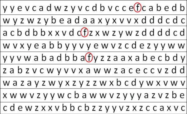
An example of a part of a training set from one of the environments. Circles (red in online version) emphasize occurrences of the reinforcer 'f’ (food). The learner receives the data as a single continuous linear sequence (illustrated in the figure as in a text page ordered from left to right, one row after the other). (Online version in colour.)

We simulated four types of environment:

• (1) Uniform environment, in which the transition probabilities between all types of elements, including food, are identical (see the electronic supplementary material, table T1).

• (2) Environment with cues for finding food, in which the transition probabilities between all non-food elements are identical, but some of them (group A: {a,b,c,d,e}) can serve as cues for the presence of food (i.e. have a non-zero probability of appearing before food), while all the others (group B: {v,w,x,y,z}) are non-cue elements in that they never occur before food (see the electronic supplementary material, table T2). The positive probability of finding an ‘f’ after one of the cues (‘a’, ‘b’, ‘c’, ‘d’ or ‘e’) was taken from a narrow gamma distribution with parameters Γ(100, 2⁻⁵). This choice of distribution leads to a clear distinction between the two groups of elements and reasonably low variance over repeated runs in the overall number of food elements in a training set.

• (3) Patchy environment, which is similar to the previous type, with the exception of being composed of patches: runs of elements of the same group (A, B). This structure is generated by setting the within-group transition probability (TP) to be higher than the between-groups TP. As a result, after an encounter with the element ‘a’ (from group A), there is a greater probability of encountering the elements ‘b’, ‘c’, ‘d’, ‘e’, (also from group A) than ‘v’, ‘w’, ‘x’, ‘y’, ‘z’ (from group B; see figures 2 and 3, and electronic supplementary material, table T3).

• (4) Directed network environment, in which the transition probabilities between any two types of elements may be non-zero and are generally not equal. The sequential patterns that can emerge under these conditions are common, for example, in natural environments with hierarchies of elements, such as a forest environment where an animal can expect the order: forest floor → tree trunk → branches → twigs → leaves. We generated and explored a number of subtypes of the directed network environment that differed in their level of entropy and in the rarity of food predictors (see the detailed description in the Results section, and references therein to TP matrices and illustrations of these various subtypes).

Figure 2.

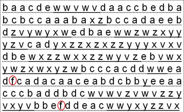
An example of a part of a training set in a patchy environment. To emphasize the patchy structure of the environment, elements that belong to the two groups (group A{a,b,c,d,e} and group B{v,w,x,y,z}) were underlined by a different line style. Circles (red in online version) mark the occurrences of the reinforcer ‘f’ (food). (Online version in colour.)

Figure 3.

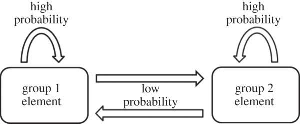
An illustration of the structure of patchy environments.

2.2. The learning models

As mentioned earlier, we modelled three types of learning mechanisms: LR, RL-chain (henceforth referred to as ‘chaining’) and CL (figure 4). In all three of them, the learner receives a sequence of elements, representing a corpus of experience of a certain foraging environment. From this, the learner constructs an internal representation, which can then be used to choose between alternatives in a simulated foraging task. As a baseline, we used a non-learner model that chooses at random.

Figure 4.

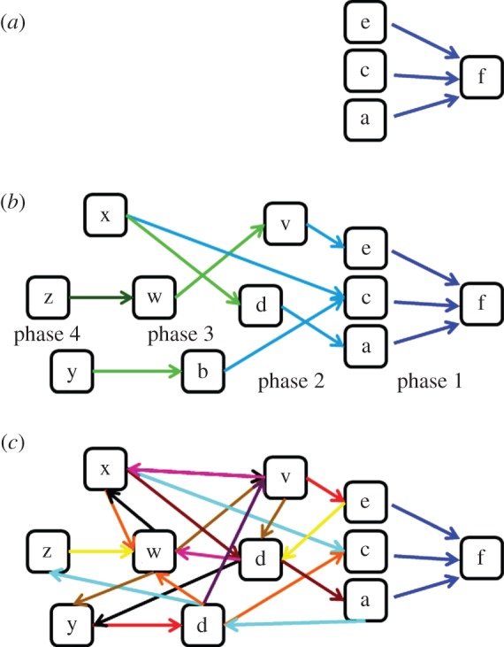
A schematic of the graph types constructed by each learning model: (a) LR, (b) RL-chain and (c) CL. Only nodes connected with links to some other nodes are shown in the figure (although all nodes encountered are monitored for their frequency of occurrence; see main text). Backward reinforcement learning (b) operates in phases, marked by different colours. In the first phase, associations between the predicting elements (cues) and the primary reinforcer are constructed. In the second phase, these predicting elements turn into secondary reinforcers and further associations can be added to them from other elements, and so on for the third and fourth phases. In the CL (c) the phases (marked with a different set of colours) may be much faster, occurring whenever data elements are encountered. Note that all links in (c) which do not involve the primary reinforcer are highly likely to be constructed before phase 1 of (b) is completed, because the primary reinforcer is typically rare, while other elements are common. Thus on completion of phase 1 by the backward chaining learner (b), the continuous learner (c) would have already constructed a full world model.

2.2.1. Model 1: local reinforcement

In this model, every encounter with an element is registered by the learner and the element is represented by a node whose weight increases linearly with each additional encounter. Yet, an association link between the element and the reinforcer (food element) is established and receives weight only when the element occurs immediately before the food element. The weight of this link increases linearly with every additional occurrence of that element immediately before the food element. The result is a simple directed graph with links leading from the learned elements (that can now be regarded as foraging cues) to the food element (figure 4a). The weights of the links represent the number of times each element was experienced immediately before food during the training period.

To choose between alternatives in a simulated foraging task (see further details in §2.3), a decision rule is applied according to which the learner always chooses the element with the highest food-finding score. This score is calculated in this case as the weight of the link between the element and the food element, divided by that element's node's weight in the graph (which represents its total number of occurrences)

2.1

Thus, the score provides a measure of the probability of finding food after the element is encountered.

2.2.2. Model 2: reinforcement learning with chaining

A learner that uses this model functions initially similar to a local reinforcement learner, but additionally, once the weight of a link between an element and the food element crosses some threshold, that element turns into a secondary reinforcer. From this point on, links between any other non-food element and the secondary reinforcer may be established and increase in weight each time the non-food element occurs immediately before the secondary reinforcer. For reasons of reliability, a non-food element can turn into a secondary reinforcement only if it has occurred at least twice, and only if the score of its link to food (or to a previously established secondary reinforcement) crosses a certain threshold. The score of this link is calculated as described in equation (2.1), representing the probability of encountering food (or a previously established secondary reinforcer) after encountering the element. The score threshold that must be crossed for an element to become a secondary reinforcer increases with the distance of this element from the original reinforcer (the food element). This setting corresponds to the notion that the strength of the reinforcement should be the strongest for the primary reinforcer and should decrease gradually along the chain (the thresholds were set to 0.004, 0.2, 0.2353, 0.2768, 0.3257, 0.3831, 0.4507, 0.5303 and 0.6239, using the formula 0.2×0.85^−(d−1) to determine all thresholds after the first one, d being the location of the secondary reinforcer along the chain). The choice of thresholds and of minimum number of occurrences for becoming a secondary reinforcer should, in a realistic setting, be adapted to the typical environment that a learner must learn; in our simulations, the thresholds were chosen so as to result in a reasonable backward chaining process. Specifically, the thresholds were set to a value that would not be too high, preventing any chaining in most simulations runs, nor too low, rendering the thresholds meaningless (turning all potential candidates into secondary reinforcers on the first encounter would make the backward chaining almost identical to CL—see below).

After the backward chaining process constructs a graph of nodes and links (figure 4b), it can be used for making foraging decisions based on the food-finding score of each element. However, this time the calculation of this score is much more complicated; it cannot be derived from equation (2.1) because it should represent the probability of finding food along the entire sequence that follows the scored element (not only the probability of finding food in the next step). To assign these scores, we used a method inspired by the spread of excitation in neural networks. An activation (of magnitude 1) is injected into the graph at the node representing the element to be scored. This propagates in the graph along the directed links. At each node, the activation is multiplied by a decay factor (0.95) and is distributed among the node's outgoing links, in proportion to each link's relative weight. An activation that drops below a certain threshold (0.05) stops propagating. Once all activations have stopped, those that arrived at the primary reinforcer node (food) are added together, and the sum is assigned to the initial element as its score. This heuristic forms an estimate of the probability that a reinforcer (food) will be found in the sequence of elements following the scored element.

2.2.3. Model 3: continuous learning

A continuous learner creates associations between any two adjacent elements as these are encountered, without regard to whether or not they are reinforcers. As in the two previous cases, the world representation that ensues is a directed graph over nodes that represent elements in the environment (figure 4c). The algorithm used to assign a food-finding score to nodes in the graph is the same excitation spread process as described above for the chaining model.

It is reasonable to assume that constructing a world model (either by chaining or by CL) requires more memory and computation than using simple reinforcement learning. However, because the magnitude of this cost and its effect on fitness are not clear, we compared the success of the three learning models assuming no differential cost in memory or computation. Our results may therefore set the minimal requirements for chaining and CL to be more successful than purely local reinforcement (see Discussion).

2.3. Training and test procedure

In each simulation, a learner was trained on a particular environment, and then tested for its foraging success in this environment. We repeated the simulation 500 times for each environment type or subtype. For each simulation run, an independent set of rules (a TP matrix) that define the environment were constructed. This was done by populating the TP matrix with randomly drawn TPs, drawn from the proper distribution (see the Results section for details regarding each environment and the electronic supplementary material, tables T1–T11 for specific examples). Using the TP matrix, a training set was generated: an initial element was chosen at random, and then each successive element was chosen probabilistically, based on the TPs from the previous element. Except where noted otherwise, all training sets were composed of 4000 elements, among which typically between 2 and 7 were food elements (the mean number of food elements in each training set was 4.5±0.25). A test set prepared for each simulation run consisted of a large number (2000, unless noted otherwise) of four-element sequences generated using the same TP matrix used to generate the training environment.

In each simulation, each learner was provided first with the training set as input. After training, the learner was presented with the 2000 test sequences. The learner could only ‘see’ the first element of each test sequence and had to choose the most promising 1000 sequences based on the food-finding score of the first element. The success rate of a learner in each simulation was defined as the total number of food elements that occurred in the sequences it chose, divided by the total number of food elements that occurred in the test set (sequences in which the first element happened to be food were not taken into account and runs in which the entire test set contained no food elements were also omitted).

We compared the success rates of the three learning models in relation to each other and in relation to the baseline (random choice) model. In each simulation, all three learning mechanisms were trained and tested with copies of the training corpus and the test set that were drawn from the probability distribution especially for that simulation. We ran 500 simulations under each condition (set of parameter values) as described later. The training corpus and test sets in each simulation were unique, and thus the statistical analyses we conducted were two-tailed paired t-tests between each two learners. Unless noted otherwise, all ‘statistically significant differences’ refer to paired t-tests with N = 500, d.f. = 498 and p < 0.0001, which remained highly significant also when controlling for multiple testing.

3. Results

3.1. Uniform environment

As expected, when the environment is uniform, no learner had an advantage over another learner or over the baseline random-choice model (figure 5a). This result confirms that when there are no cues or other regularities in the environment that can aid foraging, learning by all three models is not adaptive. It also confirms that no model has a built-in advantage or disadvantage owing to some programming artefacts or other factors unrelated to learning as such. The results remained the same with a training set of 10 000 characters (see electronic supplementary material, figure S1).

Figure 5.

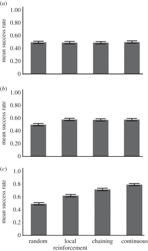
The success rate of the three types of learners and a non-learner (random choice) in: (a) uniform environment (see related TP matrix in the electronic supplementary material, table T1), (b) environment with cues for finding food (see related TP matrix in the electronic supplementary material, table T2) and (c) patchy environment (see related TP matrix in the electronic supplementary material, table T3). Success rate was calculated as the total number of food items found in the 1000 chosen sequences out of the total number of food items in the test set (2000 sequences of four characters). The bars represent the means and 95% CIs over 500 runs.

3.2. Environment with cues for finding food

In this environment, all three learners foraged with significantly higher efficiency than the random-choice baseline (paired t-tests, t₄₉₈ > 5.45, p < 0.0001 in all cases) but no learner was better than the other (figure 5b). Thus, all three learners were equally successful, showing no advantage for constructing a world model through chaining or CL. This result demonstrates a case where learning is clearly adaptive but because the only useful regularities in the environment are local, no further elaboration beyond LR is necessary. We ran the simulation with a training set of 10 000 elements to ensure sufficient time for learning, and the results remained the same (see electronic supplementary material, figure S2).

3.3. Patchy environment

In the patchy environment (figure 5c), all learners outperformed the non-learner baseline and there were significant differences among the three: RL-chain was significantly better than LR, and CL was significantly better than RL-chain (p < 0.0001 in all cases, see above).

Recall that in the patchy environment, the elements of group A ({a,b,c,d,e}) are more likely to lead to food, both directly, as ‘f’ is more likely to occur after an element of group A, and indirectly, as elements of each group are reliable predictors of one another. This helps to explain the present result: the LR may eventually reach the optimal foraging rule, after experiencing multiple instances in which each of the different elements of group A preceded the food element. If food is rare, this takes a long time. The RL-chain learner is similarly limited in its first phase of learning, but once some elements of group A are associated with food, other elements of this group quickly become secondary reinforcers and can be used to identify the correct patch even if they had never occurred immediately before food. This can explain why RL-chain is more successful than the LR. Finally, the CL is expected to be the fastest; from the beginning of the training phase, it collects data that allow it to uncover associations between food and non-food elements, as well as between different non-food elements. This logic predicts that a longer training phase, or more frequent food elements, would decrease and eventually eliminate the difference in success rate among the learners, which we confirmed through additional simulations (see the electronic supplementary material, §4).

3.4. Directed network environment

3.4.1. Constructing different subtypes of the directed network environment

We simulated four subtypes of the directed network environment. A significant dimension on which these subtypes differed is the entropy of the network: the variance among transition probabilities, which determines the predictability of paths through the network (we use the term ‘entropy’ here informally to refer to a measure of orderliness of a network; see [28]). In a high-entropy network, the probability of all trajectories of a given length is similar, whereas in a low-entropy network, certain trajectories are much more likely than the others.

Another dimension along which the directed graph subtypes differed is in the frequency of the reliable predictor of food—the one most likely to turn into a secondary reinforcer. In nature, not only is the reinforcer itself sometimes rare, but in many cases its most immediate and reliable predictors are rare as well (the footprint or the smell of prey, for example).

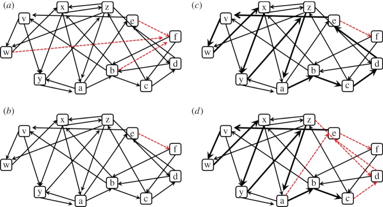
The four directed network subtypes are illustrated in figure 6. Concrete examples of each are provided in the electronic supplementary material as probability matrices (see electronic supplementary material, tables T5, T7, T8 and T10). The first subtype, a high-entropy network (figure 6a), was implemented by allowing all transitional probabilities (TPs) among non-food elements to differ from one another, by randomly drawing them from an exponential distribution (see the electronic supplementary material, §5.1 for details).

Figure 6.

An illustration of directed graphs representing regularities governing the four subtypes of web environments: (a) high-entropy network, (b) high-entropy network with a bottleneck, (c) low-entropy network and (d) a network with low entropy and rare predictors of the reinforcer. Note that in all subtypes, an edge links every two elements in the network but for the sake of clarity most edges do not appear in the illustration. Edges marked by a dotted (red in online version) line denote a low probability occurrence that may lead to a food element. Edges in bold denote probabilities that are on average greater by two orders of magnitude than the other transition probabilities. See the results section for details regarding the differences among the four environment types, and see the electronic supplementary material for examples of TP matrices that represent each type. (Online version in colour.)

In the second network subtype (figure 6b: high-entropy network with a bottleneck), we did the same, using an exponential distribution for the TPs, but also determined that besides the element ‘e’, all non-food elements would have a zero probability of preceding ‘f’ (food), while the element ‘e’ would have a positive small probability of preceding it, so that the mean number of ‘f’ occurrences in each training set would be as before (see the electronic supplementary material, table T7 for a typical TP matrix example). Thus, ‘e’ was the only direct predictor of food, but links between all other non-food elements may be learned in order to navigate to ‘e’. This feature of the graph is realistic in many real-life foraging tasks, but precludes high foraging success based on LR alone (because the number of test sequences where ‘e’ is the first element is, on average, only around 10%).

To produce a directed network with low entropy (figure 6c), we applied the same principles described above but also formed a dominant trajectory among the elements in the TP matrix. This was done by increasing the probabilities of moving along the chain: v → w → x → y → z → a → b → c → d → e to be approximately 100 times greater than the background TPs in the network (see bold arrows in figure 6c, and the electronic supplementary material, table T8).

Finally, to produce a low-entropy network with rare predictors of food, we combined the low-entropy condition with a situation in which ‘e’ and ‘d’, the closest predictors of food, were also rare (figure 6d). This was done by dividing all the TPs leading to ‘d’ and ‘e’ from all other non-food elements by 75 (before normalizing the TP matrix; see the electronic supplementary material, table T10 as an example).

3.4.2. Learning performance in high-entropy environments

When the directed graphs representing the environment had a high entropy, the differences in foraging success among the three learners were small (figure 7a). Their improvement over the baseline should be attributed mainly to learning of the local dependency between elements ‘e’ and ‘f’. The network-constructing learners (RL-chain and CL) were not more successful than LR. A possible reason for this is that although the TPs among elements were different from each other, and some routes in the network were more likely to lead to food than others, when entropy is high, even perfect knowledge of the TPs allows only limited predictive power. This explanation is supported by a set of 500 simulations in which the training set was extremely long: 50 000 elements (see the electronic supplementary material, §5.2)

Figure 7.

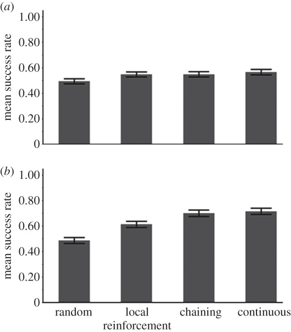
The success rate of the three types of learners in high-entropy environments, in which all elements have a certain probability of leading to ‘f’. The variance in the TPs among the elements is higher in (b) than in (a). The advantage of chaining and of CL over local reinforcement in (b) but not in (a) suggests that a high-entropy network does not offer an advantage to model-constructing learners, but networks with a somewhat lower entropy do. The difference between the chaining and the continuous learners in (b) is marginally significant and increases when training is shorter (see the electronic supplementary material, figure S4b). See related TP matrices in the electronic supplementary material, tables T5 and T6.

To decrease slightly the entropy of the graph, we generated a similar environment, while drawing the TPs from a gamma distribution, leading to higher variance among them (see the electronic supplementary material, table T6). The results in this case (figure 7b) show that RL-chain and CL performed significantly better than LR, suggesting that they could take advantage of inferring the probability of encountering food along routes in the network and not only of local regularities. Moreover, in this environment, when training was shortened to only 2000 elements, CL had a significant advantage over RL-chain (see the electronic supplementary material, §5.3).

3.4.3. Learning performance in high-entropy networks with bottlenecks

When the directed graph had a ‘bottleneck’ in the form of a single element (‘e’) that could precede food (‘f’; figure 6b), there were significant differences in foraging success among the three learners (figure 8). The learners that construct a model of the environment (RL-chain and CL) were clearly better than LR (paired t-tests, t₄₉₈ = 7.45, 9.41; p < 0.0001 in both cases). Between them, CL was the best, although only marginally so (paired t-test, t₄₉₈ = 2.66; p = 0.0081). CL's advantage was larger when the training set was shortened to 2000 elements (see electronic supplementary material, figure S5, p < 0.0002), demonstrating that the advantage of CL over RL-chain in this environment stems from its speed.

Figure 8.

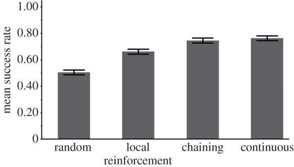
The success rate of the three learners in a high-entropy directed network with a bottleneck: transition probabilities among all elements are as in the environment in figure 7a, but the only element that leads to the reinforcer (‘f’) is ‘e’ (see illustration in figure 6b and related TP matrix in the electronic supplementary material, table T7). The continuous learner has a marginally significant advantage over the chaining learner, which becomes more significant when the training set is shortened (see the electronic supplementary material, figure S5).

3.4.4. Learning performance in directed networks with low entropy

In environments derived from a network that is highly structured and contains a bottleneck (figure 6c), we found the same trend as before: RL-chain and CL were significantly more successful than LR (figure 9a), and CL had a large advantage over RL-chain when the training set was shortened to 2000 elements (figure 9b). When we extended the training set to 24 000 characters or increased the ‘f’ frequency, we found, as expected, that the differences between these learners decreased (see electronic supplementary material, figures S6a, S6b and table T9). It is important to note that extending the training set, or increasing the frequency of food occurrence in it, did not help LR as it did in the patchy environment (compare to electronic supplementary material, figures S3a, S3b). The reason for this is that in this type of environment the occurrence of food can be inferred reliably from elements that are typically found a number of elements ‘upstream’ from it and disregarding this information is costly.

Figure 9.

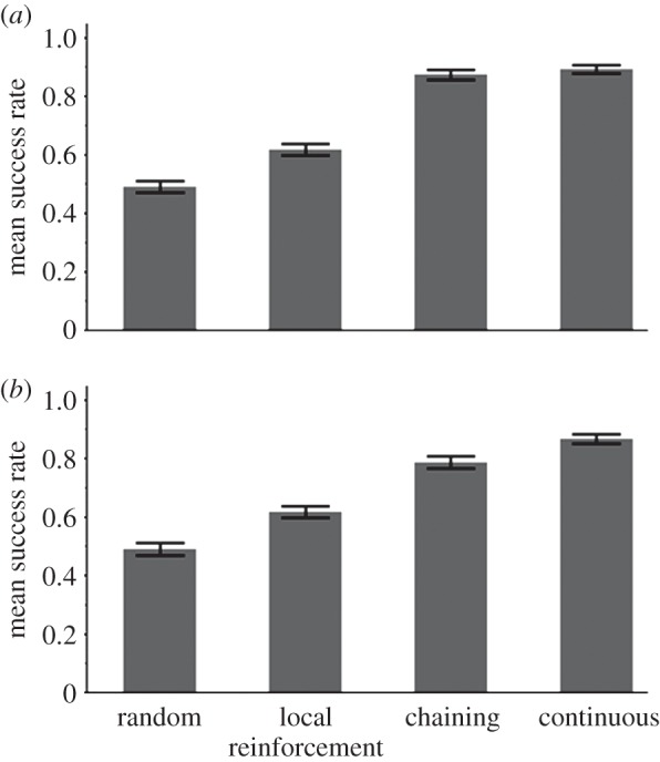
The success rate of the three learners in a low-entropy (highly ordered) network: a dominant trajectory among the elements in the network occurs with a high frequency, allowing high-accuracy prediction by model-constructing learners, thus giving a significant advantage to chaining and CL. CL has a significant advantage over chaining when the training set is shortened from 4000 to 2000 characters, (a) and (b), respectively. See related TP matrix in the electronic supplementary material, table T8.

3.4.5. Learning performance in low-entropy networks with rare predictors of food

In an environment that is structured and in which not only the food is rare but also its predictors (figure 6d), there is an advantage to RL-chain and CL over LR and a large advantage—greater than those seen previously—to CL over RL-chain (figure 10a). This is because CL, which takes advantage of all encountered data, is much faster than the gradual backward construction of a graph, which is severely limited when the key elements are all rare. Even extending the training set to 16 000 elements or increasing the frequency of food occurrence by a factor of 25 did not significantly alter this outcome (figure 10b,c), because the rarity of local predictors maintains a bottleneck for the chaining process.

Figure 10.

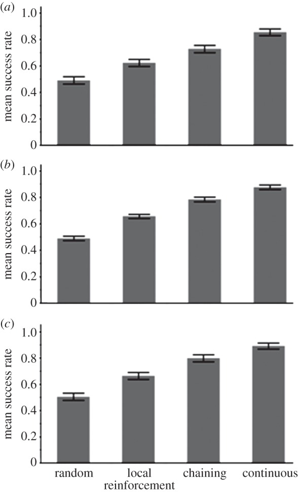
(a) The success rate of the three learners and a non-learner (random choice) in a low-entropy (highly ordered) network, with rare predictors of food (see related TP matrix in the electronic supplementary material, table T10). (b), (c) The success rate of the three types of learners and a non-learner (random choice) in a low-entropy environment with rare predictors of food, but with a high frequency of ‘f’ (b, 25 times greater than standard runs; see related TP matrix in the electronic supplementary material, table T11) or with a long training set (c, 16 000 characters; see related TP matrix in the electronic supplementary material, table T10).

4. Discussion

In this study, we explored the possible reasons for an evolutionary transition from strictly reinforced to continuous, rarely reinforced, learning. We focused on animal foraging, for which reinforcement learning is typically applied and where the goal of learning is clearly defined [29]. Using the foraging paradigm, we identified conditions under which individuals that learn the environment in a continuous manner, regardless of food findings, can nevertheless find more food items than those that rely on reinforcement learning. Moreover, all our models of learning were based on the same mechanistic building blocks of associative learning and differed only in the rules governing the acquisition of new data. Thus, our results point to a specific characteristic of the learning process on which natural selection can act in generating the evolutionary transition from reinforced to CL, or vice versa, depending on environmental conditions. At the proximate level, the transition to CL may be achieved by assigning relevance not only to data items that are in close proximity to the reinforcer but also to continuous streams of data, for example those observed along the animal's path of movement [9]. Then, the mere detection of repeated elements and regularities in the data streams may in itself evolve to be rewarding [9,26].

In what follows, we discuss some aspects of the simulation results and their possible implications.

4.1. The conditions for the evolution of continuous learning

We compared the success of CL with that of LR and RL-chain (or chaining) in a set of simulated foraging environments. The comparison with chaining was important for teasing apart the advantage stemming from constructing a world model in general and the advantage of constructing such a model in a continuous, non-reinforced fashion. As mentioned earlier, because we did not assign costs to memory and computation in our simulations, our results set the minimal requirements for the success of backward chaining and CL (see also §4.3).

We identified two main factors favouring the evolution of CL: structured environment and limited time for training. The structured environment gives advantage to model-constructing learners that can then predict the presence of food more than one step ahead. Thus, a structured environment favours both CL and RL-chain. However, the limited time for training gives CL an advantage over RL-chain because CL learners construct their world model much faster; they acquire data and construct a network right from the outset, without waiting for multiple encounters with food. As expected and confirmed by our simulations, this advantage increases when food or its most reliable predictors are rare. It is important to note that the advantage of faster model construction may be realized not only when a well-defined time window for training is limited (as in our simulations). In the real world, food depletion by other foragers is extremely common and a competitive head start is highly advantageous [30,31]. In such competitive situations, time for learning is in practice almost always limited, and therefore if the environment is sufficiently structured to justify modelling, it is probably more adaptive to construct the model through CL. Evolutionary simulations in which the various learners would actually compete with each other may further elucidate the role of competition and population dynamics in the evolution of the learning mechanisms considered here. While such simulations are beyond the scope of this paper they certainly offer an interesting direction for future work. In particular, such simulations may be useful in exploring the conditions under which a stable polymorphism of more than one learning strategy may emerge.

In addition to the main findings discussed above, our simulations yielded a few less intuitive results that are important to consider:

• (a) Not every type of highly structured environment favours model-constructing learners. In the patchy environment, for example, we found that given enough time or frequent food elements, LR was as successful as CL or RL-chain. The patchy environment is structured, but it is structured in a way that requires a forager only to identify whether a data item belongs to one patch type or another. Given sufficient time to experience food in the vicinity of each of the other elements, LR learners can obtain this information (see the electronic supplementary material, figure S3). Their representation of the world would be simple but sufficient for making the necessary foraging decisions. This result suggests that for animals that live in a stable patchy environment, LR may be good enough.

• (b) Model-constructing learners are favoured only if the environment is ‘sufficiently’ structured. Our results show that LR learners can be as successful as model-constructing learners also when the environment is somewhat structured but not structured enough, i.e. when the network's entropy is high. Although, intuitively, a structured environment is expected to favour model-constructing learners, in §3.4.2 we showed that if the entropy of a directed network environment is high, even perfect knowledge of the statistical regularities of the environment may not improve foraging success. This is because the probabilities of finding food along different paths in the network are quite equal, making chance events more influential than the ability to act according to these probabilities. In nature, we believe, many environments are structured and may be best characterized as directed network environments. Yet, it is quite possible that many of these networks are not sufficiently structured to make model construction sufficiently effective. Moreover, given that model construction may also incur costs in terms of memory and computation, not every structured environment would favour it; the environment must be sufficiently structured that the predictive power of the model improves foraging success to the extent that it outweighs the costs of constructing and managing a world model.

• (c) In strongly directed network environments, model construction is better even when food is common and the time for learning is unlimited. We already stressed the advantage of model-constructing learners in strongly directed network environments but it is still worth noting that this advantage over LR persisted even when food items were common and the learning period was in practice unlimited (see §3.4.4). The reason for this is that orderly structured environments contain useful information for finding food that cannot be learned by LR. This implies that even when the environment is stable and organisms are long lived, if the environment is also structured as a strongly directed network, LR learners will be displaced by model-constructing learners.

When considering the above-mentioned types of learning, it is important to bear in mind that for the same individual it may still be adaptive to use different learning strategies for different tasks or domains. For example, it is possible that a visual search for food in the forest may be best supported by CL of the statistical regularities of the forest environment, while searching for food by scent may be best served by local reinforcement. This is to be expected if the visual environment is structured while the olfactory environment is either patchy or insufficiently structured. Thus, a prediction of our study that may be tested by future empirical work is that the type of learning applied for different tasks or domains should be related to the statistical properties of the data available to the learner in these domains. Note that we distinguish between the statistical properties of the acquired data (see [9]) and that of the real environment, because dogs, for example, may be able to sense the complex structure of an olfactory environment that will be perceived by humans as poorly structured or patchy.

4.2. Further benefits of continuous learning

There are several benefits of CL that were not demonstrated explicitly by our simulations but can be inferred from them indirectly. First, the advantage of CL when time for learning is limited implies that it will also be advantageous in environments whose structure is changing, either seasonally, periodically, or as a result of habitat loss or succession. This should also be the case for organisms that frequently change their environment as a result of migration or dispersal. Obviously, if changes are too frequent and the learning period is therefore too short, any learning is likely to fail [32], especially learning that is more complex [4]. However, our results suggest that given a certain level of environmental complexity, CL is always faster than chaining, implying that it is likely to succeed under a wider range of changing environments.

The second potential benefit of CL is the ability to adapt quickly to changes in the behavioural goal, for example, when switching to a new type of food. Because continuous learners construct a more complete world model, and not only goal-directed chains, which lead to a particular reinforcer, they can quickly use regularities that previously had no direct use but had been learned nonetheless. When a new type of reinforcer is introduced, learning its association with only one or two items that are already represented in the network would immediately provide multiple cues for searching it from almost anywhere in the environment.

Finally, our foraging model can also be applied to the case of predator avoidance and fear learning [33,34]. The main difference is that instead of learning to navigate to the reinforcer, animals will now learn to navigate away from it, as it represents a source of danger or the location of a predator. Most importantly, in this case, CL is expected to be better than chaining because not only it is faster, but also any encounter with the reinforcer is potentially dangerous.

4.3. The costs and challenges of continuous learning as a driving factor in cognitive evolution

As mentioned earlier, our model did not assign cost to memory and computation, and therefore only set the minimal conditions for the evolution of CL. The prevalence of CL in nature (see Introduction) suggests that at least on several occasions in the course of evolution, its benefits exceeded the costs. The amount of data that can be acquired by the sensory system is typically enormous, making memory and computation extremely challenging issues to a continuous learner [24]. Moreover, the acquisition of continuous streams of data presents the challenges of segmenting the input into the most useful units [35,36] and of constructing the model in a way that would facilitate efficient search, as well as appropriate decision-making and planning [37,38]. It is therefore expected that right from the start, the evolution of CL would give rise to new selective pressures acting towards reducing the costs of memory and computation, improving the management and use of the model, and minimizing the acquisition and storage of unnecessary data. In short, the transition to CL selects for the evolution of relatively advanced cognitive mechanisms.

In this study, we simulated only simplified environments with a relatively small number of discrete data units, bypassing the above-mentioned challenges of data segmentation and complex statistical regularities. Elsewhere [20], we successfully used an extended version of our model to replicate empirical results from human language acquisition, including those involved in word segmentation, syntax learning and sentence production. We therefore suggest that modelling the evolution of CL from its most basic forms (as we did here) to elaborate ones [20,26,39] offers a biologically plausible framework for studying the incremental evolution of advanced cognition from its basic associative elements [9,40–42]. In theory, the rapid transition from reinforced to continuous, rarely reinforced, learning that can then select for more complex cognitive mechanisms could have taken place almost as early as the evolution of associative learning itself, possibly near the Cambrian explosion [43,44]. If this understanding is correct, CL and its resulting cognitive structures may be much more common than implied by current knowledge of behavioural and neural mechanisms (see [41] for the case of insects). Evidence for CL may nevertheless be revealed by different responses to familiar and novel items that have no reward value (as in [17]), or by showing a preference for such items that cannot be explained by local reinforcement or chaining.

Funding statement

O.K. was partially supported by a Dean's scholarship from the Faculty of Life Sciences at Tel-Aviv University and by a Wolf Foundation award. A.L. and O.K. were partially supported by the Israel Science Foundation grant no. 1312/11.

References

- 1.Pearce JM, Bouton ME. 2001. Theories of associative learning in animals. Annu. Rev. Psychol. 52, 111–139. ( 10.1146/annurev.psych.52.1.111) [DOI] [PubMed] [Google Scholar]
- 2.Erev I, Roth AE. 1998. Predicting how people play games: reinforcement learning in experimental games with unique, mixed strategy equilibria. Am. Econ. Rev. 88, 848–881. [Google Scholar]
- 3.Thorndike EL. 1911. Animal intelligence: experimental studies. New York, NY: Macmillan. [Google Scholar]
- 4.Arbilly M, Motro U, Feldman MW, Lotem A. 2010. Co-evolution of learning complexity and social foraging strategies. J. Theor. Biol. 267, 573–581. ( 10.1016/j.jtbi.2010.09.026) [DOI] [PMC free article] [PubMed] [Google Scholar]
- 5.Trimmer PC, McNamara JM, Houston AI, Marshall JAR. 2012. Does natural selection favour the Rescorla–Wagner rule? J. Theor. Biol. 302, 39–52. ( 10.1073/pnas.0812513106) [DOI] [PubMed] [Google Scholar]
- 6.Ferster CB, Boren MCP. 1968. Behavior principles. New York, NY: Appleton-Century-Crofts. [Google Scholar]
- 7.Millenson JR. 1967. Principles of behavioral analysis. New York, NY: Macmillan. [Google Scholar]
- 8.Skinner BF. 1966. The behavior of organisms. New York, NY: Appleton-Century-Crofts. [Google Scholar]
- 9.Lotem A, Halpern JY. 2012. Coevolution of learning and data-acquisition mechanisms: a model for cognitive evolution. Phil. Trans. R. Soc. B 367, 2686–2694. ( 10.1098/rstb.2012.0213) [DOI] [PMC free article] [PubMed] [Google Scholar]
- 10.Fonio E, Benjamini Y, Golani I. 2009. Freedom of movement and the stability of its unfolding in free exploration of mice. Proc. Natl Acad. Sci. USA 106, 21 335–21 340. ( 10.1073/pnas.0812513106) [DOI] [PMC free article] [PubMed] [Google Scholar]
- 11.Bateson P, Young M. 1979. Influence of male kittens on the object play of their female siblings. Behav. Neural Biol. 27, 374–378. ( 10.1016/S0163-1047(79)92468-3) [DOI] [PubMed] [Google Scholar]
- 12.Barrett P, Bateson P. 1978. Development of play in cats. Behaviour 66, 106–120. ( 10.1163/156853978X00422) [DOI] [Google Scholar]
- 13.Auersperg AMI, Gajdon GK, Huber L. 2009. Kea (Nestor notabilis) consider spatial relationships between objects in the support problem. Biol. Lett. 5, 455–458. ( 10.1098/rsbl.2009.0114) [DOI] [PMC free article] [PubMed] [Google Scholar]
- 14.Diamond J, Bond AB. 2004. Social play in kaka (Nestor meridionalis) with comparisons to kea (Nestor notabilis). Behaviour 141, 777–798. ( 10.1163/1568539042265680) [DOI] [Google Scholar]
- 15.Dingemanse NJ, Both C, Drent PJ, Van Oers K, Van Noordwijk AJ. 2002. Repeatability and heritability of exploratory behaviour in great tits from the wild. Anim. Behav. 64, 929–938. ( 10.1006/anbe.2002.2006) [DOI] [Google Scholar]
- 16.Archer J, Birke LIA. 1983. Exploration in animals and humans. Wokingham, UK: Van Nostrand Reinhold (UK). [Google Scholar]
- 17.Heinrich B. 1995. Neophilia and exploration in juvenile common ravens, Corvus corax. Anim. Behav. 50, 695–704. ( 10.1016/0003-3472(95)80130-8) [DOI] [Google Scholar]
- 18.Pisula W. 2009. Curiosity and information seeking in animal and human behavior. Boca Raton, CA: Brown Walker Press. [Google Scholar]
- 19.Valone TJ. 2007. From eavesdropping on performance to copying the behavior of others: a review of public information use. Behav. Ecol. Sociobiol. 62, 1–14. ( 10.1007/s00265-007-0439-6) [DOI] [Google Scholar]
- 20.Kolodny O, Lotem A, Edelman S. In press. Learning a generative probabilistic grammar of experience: a process-level model of language acquisition. Cogn. Sci. [DOI] [PubMed]
- 21.Edelman S, Waterfall HR. 2007. Behavioral and computational aspects of language and its acquisition. Phys. Life Rev. 4, 253–277. ( 10.1016/j.plrev.2007.10.001) [DOI] [Google Scholar]
- 22.ten Cate C, Okanoya K. 2012. Revisiting the syntactic abilities of non-human animals: natural vocalizations and artificial grammar learning. Phil. Trans. R. Soc. B 367, 1984–1994. ( 10.1098/rstb.2012.0055) [DOI] [PMC free article] [PubMed] [Google Scholar]
- 23.Gottlieb J, Oudeyer PY, Lopes M, Baranes A. 2013. Information-seeking, curiosity, and attention: computational and neural mechanisms. Trends Cogn. Sci. 17, 585–593. ( 10.1016/j.tics.2013.09.001) [DOI] [PMC free article] [PubMed] [Google Scholar]
- 24.Harris ZS. 1991. A theory of language and information. Oxford, UK: Clarendon Press. [Google Scholar]
- 25.Tenenbaum JB, Kemp C, Griffiths TL, Goodman ND. 2011. How to grow a mind: statistics, structure, and abstraction. Science 331, 1279–1285. ( 10.1126/science.1192788) [DOI] [PubMed] [Google Scholar]
- 26.Goldstein MH, Waterfall HR, Lotem A, Halpern J, Schwade J, Onnis L, Edelman S. 2010. General cognitive principles for learning structure in time and space. Trends Cogn. Sci. 14, 249–258. ( 10.1016/j.tics.2010.02.004) [DOI] [PubMed] [Google Scholar]
- 27.Norris JR. 1997. Markov chains. New York, NY: Cambridge University Press. [Google Scholar]
- 28.Mowshowitz A, Dehmer M. 2012. Entropy and the complexity of graphs revisited. Entropy 14, 559–570. ( 10.3390/e14030559) [DOI] [Google Scholar]
- 29.Stephens DW, Dunlap AS. 2008. Foraging. In Learning and memory: a comprehensive reference (ed. Menzel R.), pp. 365–384. Oxford, UK: Elsevier. [Google Scholar]
- 30.Krebs JR, Davies NB. 1987. An introduction to behavioral ecology. Oxford, UK: Blackwell. [Google Scholar]
- 31.Fretwell SD, Lucas HLJ. 1969. On territorial behavior and other factors influencing habitat distribution in birds. Acta Biotheor. 19, 16–36. ( 10.1007/BF01601953) [DOI] [Google Scholar]
- 32.Stephens DW. 1991. Change, regularity, and value in the evolution of animal learning. Behav. Ecol. 2, 77–89. ( 10.1093/beheco/2.1.77) [DOI] [Google Scholar]
- 33.Webster MM, Laland KN. 2008. Social learning strategies and predation risk: minnows copy only when using private information would be costly. Proc. R. Soc. B 275, 2869–2876. ( 10.1098/rspb.2008.0817) [DOI] [PMC free article] [PubMed] [Google Scholar]
- 34.Ydenberg RC. 1998. Behavioral decisions about foraging and predator avoidance. In Cognitive ecology: the evolutionary ecology of information processing and decision making (ed. Dukas R.), pp. 343–378. Chicago, IL: University of Chicago press. [Google Scholar]
- 35.Gobet F, Lane PCR, Croker S, Cheng PCH, Jones G, Oliver L, Pine JM. 2001. Chunking mechanisms in human learning. Trends Cogn. Sci. 5, 236–243. ( 10.1016/S1364-6613(00)01662-4) [DOI] [PubMed] [Google Scholar]
- 36.Terrace H. 2001. Chunking and serially organized behavior in pigeons, monkeys and humans. In Avian visual cognition (ed. Cook RG.). See http://www.pigeon.psy.tufts.edu/avc/terrace/. [Google Scholar]
- 37.Anderson JR. 1993. Rules of the mind. Hillsdale, MI: Erlbaum. [Google Scholar]
- 38.Gallistel CR. 2008. Learning and representation. In Learning theory and behaviour (ed. Menzel R.), pp. 227–242. Oxford, UK: Elsevier. [Google Scholar]
- 39.Solan Z, Horn D, Ruppin E, Edelman S. 2005. Unsupervised learning of natural languages. Proc. Natl Acad. Sci. USA 102, 11 629–11 634. ( 10.1073/pnas.0409746102) [DOI] [PMC free article] [PubMed] [Google Scholar]
- 40.Jacobs LF. 2012. From chemotaxis to the cognitive map: the function of olfaction. Proc. Natl Acad. Sci. USA 109(Suppl. 1), 10 693–10 700. ( 10.1073/pnas.1201880109) [DOI] [PMC free article] [PubMed] [Google Scholar]
- 41.Webb B. 2012. Cognition in insects. Phil. Trans. R. Soc. B 367, 2715–2722. ( 10.1098/rstb.2012.0218) [DOI] [PMC free article] [PubMed] [Google Scholar]
- 42.Cook R, Bird G, Catmur C, Press C, Heyes C. In press Mirror neurons: from origin to function. Behav. Brain Sci. [DOI] [PubMed] [Google Scholar]
- 43.Ginsburg S, Jablonka E. 2010. The evolution of associative learning: a factor in the Cambrian explosion. J. Theor. Biol. 266, 11–20. ( 10.1016/j.jtbi.2010.06.017) [DOI] [PubMed] [Google Scholar]
- 44.Trestman M. 2013. The Cambrian explosion and the origins of embodied cognition. Biol. Theory 8, 80–92. ( 10.1007/s13752-013-0102-6) [DOI] [Google Scholar]