Measurement of the toughness of bone: A tutorial with special reference to small animal studies

Abstract

Quantitative assessment of the strength and toughness of bone has become an integral part of many biological and bioengineering studies on the structural properties of bone and their degradation due to aging, disease and therapeutic treatment. Whereas the biomechanical techniques for characterizing bone strength are well documented, few studies have focused on the theory, methodology, and various experimental procedures for evaluating the fracture toughness of bone, i.e., its resistance to fracture, with particular reference to whole bone testing in small animal studies. In this tutorial, we consider the many techniques for evaluating toughness and assess their specific relevance and application to the mechanical testing of small animal bones. Parallel experimental studies on wild-type rat and mouse femurs are used to evaluate the utility of these techniques and specifically to determine the coefficient of variation of the measured toughness values.

Introduction

There are numerous studies that have investigated the effects of age, drug treatments and disease on the structure and properties of bone [1-11]. Many of these studies employed mechanical testing to evaluate how the structural properties of the bone are affected. Of these, the fundamental structural properties of greatest importance are generally the stiffness, strength and toughness, together with more complicated properties such as the fatigue resistance. Biomechanical testing to evaluate the stiffness, which is defined in terms of the elastic modulus (generally Young’s but sometimes shear), and the strength (assessed in terms of the hardness or the yield, ultimate or fracture strength tested in tension, compression, bending or shear) are well documented. For macroscopic testing, which dictates how bone will actually behave, articles by Turner and Burr [12] and more recently by Akhter et al. [13] give precise descriptions as to how these properties of bone can be quantitatively assessed, both on whole bones, such as femurs and vertebrae, and with standard specimens cut from the cortical shell. For more mechanistic evaluation, the stiffness and hardness can also be assessed for both cortical and trabecular bone at local (nano-/microscopic) dimensions using nanoindentation testing, as documented in refs. [14,15], although for biological materials, it is more difficult with this technique to get reproducible results. Indeed, Silva et al. [14] have recently found little correlation between moduli measured with nanoindentation, as compared to whole bone mechanical testing.

However, since the critical structural property of bone is arguably its fragility or more correctly its resistance to fracture, it is perhaps surprising that there have been no corresponding “tutorials” published on how similarly to evaluate the toughness of bone. Indeed, there is no standard method that has been used to assess bone toughness; historically, parameters such as the “work to fracture” (the work necessary to break a solid and form two surfaces, W_f) have been employed [16] although more recently there has been increasing use of fracture mechanics parameters, such as the fracture toughness [1,3]. Although standards exist for the methods of assessing toughness in structural materials, such as the American Society for Testing and Materials (ASTM) standards [17,18], there have been few comprehensive descriptions of their optimum application and interpretation to biological materials. In bone where test samples can be machined from the cortical shell, there have been several recent studies where various fracture mechanics test methods have been utilized to evaluate toughness; these include measurements of:

• linear-elastic fracture mechanics (LEFM) fracture toughness (K_c) [1,3,19-26]

• nonlinear-elastic fracture mechanics fracture toughness (J_c) [27,28]

• crack-resistance curves (R-curves) [6,7,28-30]

• nonlinear methods involving cohesive-zone models [31-33].

However, each of these methods assesses a different aspect of fracture resistance; i.e., K_c measurements essentially define the toughness to initiate cracking, J_c values include the additional contribution from inelastic deformation (e.g., plasticity), and R-curves are a measure of the toughness of a growing crack. Moreover, in biological studies, the strict specifications on test sample size, geometry, and configuration, and the need for an atomically-sharp starter crack, which are required to obtain “valid” results from such measurements, are not always (or often cannot be) followed.¹ For this reason, it is difficult to perform quantitative comparisons between published data from different researchers; furthermore, many of the fracture toughness (particularly K_c) measurements in the literature are size- and geometry-dependent.

For biological materials the difficulty in performing “valid” measurements is due to the physiological size limitations of the samples that can be fabricated. Because of the small sample sizes available in some bones (this is even more difficult for some orientations), achieving a state of plane strain² or satisfying the requirements to apply linear-elastic fracture mechanics can be a challenge. Generating an atomically-sharp starter crack is nontrivial because the technique of fatiguing in a starter crack requires precise control for the small biological specimen and constraint at the crack tip to prevent changes to the bulk material. This is important as the effective stress intensity developed at a notch or crack can be severely reduced if the stress concentrator is not sharp (typically the value of stress intensity K is decreased by an amount inversely proportional to the square-root of the root radius of the notch).³

The situation is even more complicated where fracture resistance testing is performed on whole bones, especially in small animal models such as rat and mouse. In these cases, as the samples are not physically large and vary in size, requirements of standard specimen sizes and geometry are all but impossible to meet, and the mechanical testing itself becomes especially challenging. This problem is compounded by the fact that there is also little information about what the expected variation in such measurements should be, which is critical to know when small animal models are used to evaluate the effects of specific therapeutic treatments, such as glucoctorticoids, bisphosphonates, etc., on the fragility of bone. Indeed, a recent study by Currey et al. [36] on the variability of mechanical properties in human, bovine, equine and various vertebrates’ bone, reported that the coefficient of variation (standard deviation/mean) for various measures of toughness, specifically the work to fracture and similar energy parameters measured in tension and impact, all exceeded 30% and were greater than all other mechanical properties (mainly stiffness and strength) considered.

Accordingly, in the current work we first describe in some detail the various test methods and parameters that can be used to assess the toughness of bone. We then discuss how these approaches can be actually applied to the toughness testing of whole bone, with special reference to small animal model studies specifically involving mouse and rat bone. Finally, we describe the results of a “large-N” study on small animal bone to evaluate the variability in toughness values measured using some of these techniques.

Strength vs. toughness

The toughness is a measure of resistance to fracture. However, before describing the various means of measuring this quantity in bone, it is worth discussing first its distinction from the more commonly measured quantity of strength. In ductile materials such as metals, this distinction is quite clear. The strength is a measure of resistance to permanent (plastic) deformation. It is defined, invariably in uniaxial tension, compression or bending, either at first yield (yield strength) or at maximum applied load (ultimate strength). In most ductile materials, high strength implies low toughness and vice versa. In contrast, in brittle materials such as ceramics where macroscopic plastic deformation is essentially absent, the strength measured in a uniaxial tensile or bending test is governed by when the sample fractures; it is not only a function of how much stress or strain that the material can endure but primarily a function of the distribution of defects, e.g., microcracks, that may be present,⁴ i.e., the fracture stress will not be a material constant like the yield strength but will depend on the size of pre-existing defects [37]. With certain older measures of toughness, such as the work to fracture, which are determined by breaking an unnotched sample, the toughness and strength may be measuring the same property (although the units are different). However, what this implies is that in all classes of material, fracture resistance does not simply depend upon simply the maximum stress or strain to cause fracture but also on the ubiquitous presence of crack-like defects and their size. Since the pre-existing defect distribution is rarely known in strength tests, the essence of the fracture mechanics description of toughness is to first precrack the test sample, with a known (nominally) atomically-sharp (worst-case) crack (generally a fatigue crack), and then to determine the stress intensity or energy required to fracture the material in the presence of this worst-case flaw (this property is termed the fracture toughness).

Bone is a brittle material which microcracks and displays some degree of inelasticity; consequently, the strength of bone will be a measure of the stress required to deform and fracture the material and will depend upon whatever flaw-like defects might be present [37]. Toughness assessed in terms of the work to fracture will measure similar properties although now in terms of an energy. The fracture mechanics based fracture toughness on the other hand will provide a measure of the toughness in the presence of a dominant flaw of known worst-case size; it is therefore a better representation of the resistance to fracture and dictates how the stress or strain to cause fracture will vary with defect size.

It should be noted that our interpretation of the meaning and significance of strength and toughness to bone does differ somewhat from previous deliberations [3]. Since specimens that assess strength are unnotched whereas fracture toughness test geometries all contain a precrack or sharp notch, the former tests invariably “probe” a larger statistical sampling volume of material. However, by initiating fracture from a pre-existing “worse-case” precrack/notch, the mechanical role of microstructural defects, specifically microcracks, is minimized [37]. As such, fracture toughness measurements characterize the inherent resistance of a material to fracture, and with such techniques as R-curve analysis (described below) can be used to separate the individual contributions from crack initiation and crack growth, which is an important distinction for bone. We would therefore contend that the evaluation of toughness, by the methods proposed in this work, has intrinsic merit that exceeds its use as a parameter to predict strength, as has been previously proposed [3].

Measurement of toughness

Work to fracture

A measure of toughness which has been used in the past to assess the toughness of bone is the so-called work to fracture, W_f [16]. This is defined as the work per unit area to break an unnotched specimen loaded in bending or tension into two pieces; it is therefore determined by the fracture energy normalized by the surface of the fracture, i.e., the area under the load/displacement curve divided by twice the area of the fracture surface.

As noted above, as the sample, is tested without any precrack or notch, this measure of toughness is essentially the energy equivalent of a fracture strength. It will depend not simply on the bone-matrix structure but also on the distribution of defects in the bone (either natural or created during specimen preparation). This method suffers from a dependence on specimen size and geometry; it is thus inadvisable to compare work to fracture data from different investigators and different studies.

Linear-elastic fracture mechanics

Fracture toughness (crack-initiation toughness)

The standard means today of quantitatively assessing the fracture resistance of most materials is to use fracture mechanics. In its simplest form, linear-elastic fracture mechanics, the material is considered to be nominally elastic, with the region of inelasticity at the crack tip, the plastic zone, remaining small compared to the (in-plane) specimen dimensions (“small-scale yielding”). The local stresses, σ_ij, at distance r and angle θ to a crack tip can be expressed (as r → 0) by σ_ij → [K/(2πr)^1/2]f_ij(θ), where f_ij(θ) is an angular function of θ, and K is the stress-intensity factor⁵, which is defined in terms of the applied stress, σ_app, crack length a, and a geometry function Q of order unity, i.e., K=Q σ_app (πa)^1/2, and represents a scalar parameter characterizing of the local stress (and displacement) fields [38]. Provided it characterizes the local stresses and strains over dimensions comparable to the scale of local fracture events, it can be deemed to reach a critical value, the fracture toughness, at fracture, K=K_c [39]. For this approach to be valid, small-scale yielding must apply, which requires the plastic zone, r_y ~ 1/2π (K/σ_y)² (σ_y is the yield strength),⁶ to be more than an order of magnitude smaller than the in-plane dimensions of crack size a, specimen width W, and remaining uncracked ligament (W–a); for plane-strain conditions to apply, the plastic zone must be similarly small compared to the out-of-plane thickness dimension B [40].

An alternative, yet equivalent, approach, which is often preferable for mixed-mode fracture, involves the strain-energy release rate, G, which is defined as the rate of change in potential energy per unit increase in crack area. Given the equivalence between K and G for linear-elastic materials [39]:

$$G=\frac{K_{\mathrm{I}}^2}{E^{\prime }}+\frac{K_{\mathrm{II}}^2}{E^{\prime }}+\frac{K_{\mathrm{III}}^2}{2\mu },$$ (1)

where μ is the shear modulus and E′ = E (Young’s modulus) in plane stress and E/(1 − ν²) in plane strain (ν is Poisson’s ratio), G_c can be also used as a measure of fracture toughness.

ASTM has developed standard test methods for measuring the plane-strain fracture toughness in mode I for metallic materials (ASTM E399-90 [17]), and by default for other materials. The most widely used specimen configurations for bone are the single-edge notched three-point bend SE(B) and compact-tension C(T) specimens (Fig. 1), where K_I is given in terms of the applied load P and loading S, respectively, as [18]:

$$K_{\mathrm{I}}=\frac{\mathit{PS}}{B{W}^{3/2}}f(a/W)\mathrm{and}{K}_{\mathrm{I}}=\frac{P}{B{W}^{1/2}}{f}^{\prime }(a/W),$$ (2)

where f(a/W) and f′(a/W) are geometric functions of a/W tabulated in ref. [18]. The critical load at crack initiation, or instability, defines the toughness K_c provided small-scale yielding conditions apply. If additionally plane-strain conditions prevail, this is termed the plane-strain fracture toughness, K_Ic, and can be considered a material property under these conditions.⁷

Fig. 1.

Schematic diagrams of mammalian long bone showing the locations where samples can be harvested from the cortex. Samples can be fabricated to test bone in the transverse or the longitudinal directions. Shown here are the SE(B) and C(T) geometries for testing the transverse and longitudinal directions respectively.

Measurements of the toughness performed in this manner are single-valued, strictly pertain to crack initiation being synonymous with instability, and do not incorporate any contribution from plastic or inelastic deformation.

Crack-resistance curve (crack-growth toughness)

In many materials, fracture instability takes place well after crack initiation due to the occurrence of subcritical crack growth, i.e., stable crack growth at K<K_c. This is a characteristic of ductile materials and also more brittle materials that are toughened extrinsically.⁸ Indeed, bone is such a material and actually develops its prime sources of toughness during crack growth [6,7,28,29,43,44]. In order to assess the crack-growth toughness, the crack-resistance curve, or R-curve, is generally determined, which entails the measurement of the crack-driving force, e.g., K or G, as a function of stable crack extension, Δa. Crack extension must be monitored; a commonly-used procedure involves measuring the elastic unloading compliance, C, and relating this to crack length from handbook solutions [18] for the particular test-piece geometry.

As the R-curve, K_R(Δa) or G_R(Δa), should be independent of the initial crack size, it can be considered as a measure of the crack-growth toughness, although the slope of the R-curve has also been referred to by this term. Fig. 2 provides a schematic of crack-growth resistance curves for a material with a flat R-curve and a rising R-curve.

Fig. 2.

Schematics of flat and rising crack-growth resistance curves (R-curves). Unstable fracture occurs when the materials resistance to fracture ceases to increase faster than the driving force for crack propagation; this corresponds to the driving force as a function of crack size being tangent to the crack-growth resistance curve. For a material that has a flat R-curve, a single value of toughness unambiguously characterizes the material. For a material with a rising R-curve there is no single value of toughness that characterizes the material as the driving force for unstable crack propagation depends on the extent of crack growth. For materials with rising R-curves crack-growth resistance, measurements are needed to determine how the resistance to fracture evolves with crack extension. For materials with flat R-curves, there is no stable crack extension and the initial crack size (a_o) is the same as the critical crack size (a_c). In materials with a rising R-curve, stable crack growth occurs and the critical crack size will be larger than the initial crack size. Crack-growth resistance curves are typically plotted with crack extension (Δa) instead of crack size because the shape of the R-curve does not vary with crack size. The driving force for crack propagation can be quantified by K, G, or J.

Nonlinear-elastic fracture mechanics

J-integral measurements

In the presence of more extensive plastic deformation, nonlinear-elastic fracture mechanics may provide an improved assessment of toughness. Here, for a material satisfying a nonlinear-elastic constitutive law relating stress σ to strain ε in the form of ε/ε_o = α (σ/σ_o)ⁿ, where σ_o and ε_o are reference values, α is a constant, and n is the strain hardening coefficient, the local stresses, σ_ij, at distance r and angle θ to a crack tip can be expressed by another unique asymptotic solution [45,46]:

$$\mathrm{as}r\to 0,{\sigma }_{\mathrm{ij}}(\theta ,n)\to \alpha {\left(\frac{J}{(\alpha {\sigma }_{\mathrm{o}}{\epsilon }_{\mathrm{o}}{I}_{n}r)}\right)}^{1/n}{f}_{\mathrm{ij}}(\theta ,n),$$ (3)

where f_ij(θ,n) is an angular function of θ and n, I_n is an integration constant, and J is the J-integral [47]. Akin to K in the linear-elastic singularity, J is the characterizing parameter for the nonlinear-elastic (HRR) singularity [45,46]; as such, it uniquely characterizes the crack-tip stress and strain fields. Provided this is true over dimensions comparable to the scale of fracture events, J also can be used as a correlator to crack initiation and growth, but now for a solid undergoing some degree of inelastic deformation. At fracture initiation, J = J_c, which can be used as a descriptor of the (crack-initiation) fracture toughness [18].

As J can also be defined as the rate of change in potential energy per unit increase in crack area for a nonlinear-elastic solid, it is equal to G under linear-elastic conditions; consequently J_c values can this be used to estimate K_c fracture toughnesses simply using Eq. (1).

ASTM has similarly developed standard test methods for measuring the J_c (or plane-strain J_Ic) fracture toughness and J_R(Δa) R-curves (ASTM E1820-06 [18]), using several standard specimen configurations, most notably the SE(B) and C(T) specimens (Fig. 1). For the three-point bending SE(B) and compact-tension C(T) configurations, J is given by [18]:

$$J=\frac{K^2}{E^{\prime }}+\frac{\eta }{B(W-a)}{A}_{\mathrm{pl}},$$ (4)

where η (a geometry factor)=2 for the SE(B) geometry and =2+0.522 (W-a)/W for the C(T) geometry, and A_pl is the area under the applied load/plastic load-line displacement plot. Typically, a J_R(Δa) R-curve is measured and then the initiation J_c (or J_Ic) value computed by extrapolating the R-curve essentially back to Δa → 0 (or to a blunting line, as described in ASTM E1820-06 [18]). There are requirements for this approach to be valid; unlike K though, they depend upon the specific specimen geometry used. For both the SE(B) and C(T) specimens, the validity of the J-field is assured if W-a>25 J/σ_f, where σ_f is the flow stress (mean of the yield and ultimate tensile strengths). Plane-strain conditions would prevail where B>25 J/σ_f, in which case the fracture toughness is termed J_Ic.

Akin to linear-elastic fracture mechanics, whereas the crack-initiation fracture toughness can be characterized in terms of J_c and J_Ic, the J_R(Δa) R-curve (or its slope, dJ_R/dΔa) provides a measure of the crack-growth toughness. However, unlike K-based measurements, J-based measurements include the important contribution of inelasticity (e.g., plastic deformation) in the quantitative assessment of the fracture toughness. This latter effect is important for bone, as has been recently demonstrated in refs. [27,28], in particular because of the occurrence of diffuse damage and microcrack formation which can act as mechanisms of inelasticity.

Toughness testing of whole bone: small animal models

Rat and mouse models

K_c fracture toughness measurements

Femurs are the ideal rat and mouse bones to evaluate the fracture toughness properties in small animal model studies. These bones are 30–40 mm long with a ~3–4 mm diameter in rats and ~15 mm long with a ~1–2 mm diameter in mice, and can be readily tested in three-point bending. The ends of the bones are best cut off with a low-speed saw, then notched and loaded such that the posterior surface is in tension and the anterior surface is in compression (Fig. 3). Slow-speed sawing is recommended through the thickness of the cortical wall in the case of a long bone, and for machining a circumferential through-wall notch. The latter can then be subsequently sharpened by “polishing” with a razor blade irrigated with 1 μm diamond suspension; this razor micronotching technique [35] results in a consistently sharp notch with a root radius of ~10 μm. All measurements need to be performed in fluid that simulates in vivo conditions, e.g., Hanks’ Balanced Salt Solution (HBSS), at 37 °C.

Fig. 3.

Schematic diagram of where the specimens were taken from the femurs. For the mice the entire shaft of the femur was used and for the rats only the half of the shaft closest to the kneewas used. Unnotched specimens were obtained in the same manner. Also shown is a schematic of the measurement of the half-crack angles. To measure the half-crack angle for the crack-initiation and maximum load methods for calculating K_c, the half-crack angle for the notch is defined in the left-hand figure. Two lines should be extended from the geometric center of the bone (located by the intersection of major and minor axes) to the edge of the notch. These lines should terminate in the middle of the cortical wall. For the fracture instability method, the same process should be applied, except the lines should terminate at the boundary of the stable crack-growth region and the unstable crack-growth region, as shown by the right-hand figure.

Since mouse and rat bones are somewhat small to generate full R-curve behavior, particularly since this would involve the very difficult task of monitoring crack extension over such small dimensions, the best alternative measure of toughness is to determine a single-valued K_c. As noted above, this involves testing the samples in three-point bending and measuring the load and crack length at crack initiation, maximum load or fracture instability. To calculate the mode I stress-intensity factor, solutions for circumferential through-wall cracks in cylindrical pipes [48,49], can be used, where the value of K_I is given in terms of the wall (bone cortex) thickness t, mean radius R_m of the bone (to middle of the cortex), and crack length, defined in terms of the half-crack angle Θ in Fig. 3:

$$K_{\mathrm{I}}=F_{\mathrm{b}}{\sigma }_{\mathrm{b}}\sqrt{\pi R_{\mathrm{m}}\Theta ,}$$ (5)

where F_b is a geometry factor and σ_b, the applied bending stress, is calculated from the bending moment M (=PS/4) in terms of the distance from the neutral axis, c, and area moment of inertia I, as σ_b=Mc/I. This solution is valid for both thin-walled and thick-walled bones, specifically for 1.5<R_m/t<80.5, and for a range of half-crack angles, 0<Θ/π<0.611. Takahashi [49] assumed a thin-walled pipe solution to compute σ_b, namely:

$${\sigma }_{\mathrm{b}}=\frac{M}{2\pi R_{\mathrm{m}}^{2}t},$$ (6)

although for applications involving femurs, a thick-walled pipe solution for the moment of inertia is more appropriate in terms of the inner, R_i, and outer, R_o, radius of the cortical shell; this gives the definition of σ_b as:

$${\sigma }_{\mathrm{b}}=\frac{M{R}_{\mathrm{o}}}{\frac{\pi }{4}(R_{\mathrm{o}}^4-R_{\mathrm{i}}^4)}.$$ (7)

Under these conditions, F_b is given by:

$$F_{\mathrm{b}}=\left(1+\frac{t}{2R_{\mathrm{m}}}\right)\left[A_{\mathrm{b}}+B_{\mathrm{b}}\left(\frac{\Theta }{\pi }\right)+C_{\mathrm{b}}{\left(\frac{\Theta }{\pi }\right)}^2+D_{\mathrm{b}}{\left(\frac{\Theta }{\pi }\right)}^3+E_{\mathrm{b}}{\left(\frac{\Theta }{\pi }\right)}^4\right],$$ (8)

where

$$\begin{array}{l}{A}_b=0.65133-0.5774\xi -0.3427{\xi }^2-0.0681{\xi }^3,\\ B_b=1.879+4.795\xi +2.343{\xi }^2-0.6197{\xi }^3,\\ C_b=-9.779-38.14\xi -6.611{\xi }^2+3.972{\xi }^3,\\ D_b=34.56+129.9\xi +50.55{\xi }^2+3.374{\xi }^3,\\ E_b=-30.82-147.6\xi -78.38{\xi }^2-15.54{\xi }^3,\\ \xi =\log \left(\frac{t}{R_{\mathrm{m}}}\right).\end{array}$$

These solutions assume a circular cross section whereas long bones generally are far less uniform. A “propagation of errors” calculation through these “thick-walled pipe” stress-intensity solutions shows that deviations of the bone dimensions away from a circular cross section with a uniform thickness have the greatest effect on the accuracy of the K-solution. An analysis of the resulting worst-case errors in computed stress-intensity values reveals an uncertainty of ~17%, as described in Appendix I.

With respect to the point on the load-displacement curve where the toughness is measured, there are several approaches that can be employed to define the critical load P_c and crack size (i.e., the half-crack angle Θ) used to compute the value of K_c (Fig. 3). For an intrinsic, crack-initiation toughness value, ideally the onset of cracking should be monitored independently and the load at crack initiation noted (crack-initiation method). As per the ASTM Standards [17], this can be estimated by noting the load P_Q at the intercept of the load/displacement curve with a 5% secant line, i.e., a line drawn from the origin with a slope 95% of the initial elastic loading line (this is intended to represent a crack extension of roughly 2% of the remaining ligament). However, for this latter (5% secant) construction to work, there must be only limited plasticity (as this also affects the compliance slope); to ensure that this is the case, the E-399 Standard [17] also requires that P_max/P_Q≤1.1 (where P_max is the maximum load) for a valid K_c result.

Due to the presence of plasticity in samples which are physically small, the 5% secant construction can be inaccurate in small animal studies. Accordingly, a more straightforward and simple way is to define instability at maximum load, P_c=P_max, and to use the length of the starter notch, a_c=a_init (Θ_c=Θ_init) as the initial crack size (maximum load method). However, the latter approach is also liable to be inaccurate due to the possibility that some degree of subcritical (stable) cracking occurs prior to instability; moreover, in actuality, crack initiation rarely takes place exactly at maximum load. Since subcritical crack growth does occur in mouse and rat femurs, an alternative, more accurate, approach is to take the load at fracture instability, P_f, and to use backscattered scanning electron microscopy (SEM) to determine the extent of subcritical cracking⁹ in order to determine the corresponding crack size at instability Θ_c=Θ_inst (fracture instability method). Fig. 4 shows an SEM image of the notch, region of stable crack growth, and the onset of overload fracture. Fig. 5 shows environmental SEM images of the stable crack profile and unstable crack profile taken in situ,¹⁰ and fractography images of each region.

Fig. 4.

SEM image showing the machined notch, region of stable crack growth, and the region of unstable fracture, used to measure the crack size (half-crack angle) for the instability method of determining the fracture toughness. This micrograph is of a mouse femur; the inset shows the region of the cortex where the image was taken.

Fig. 5.

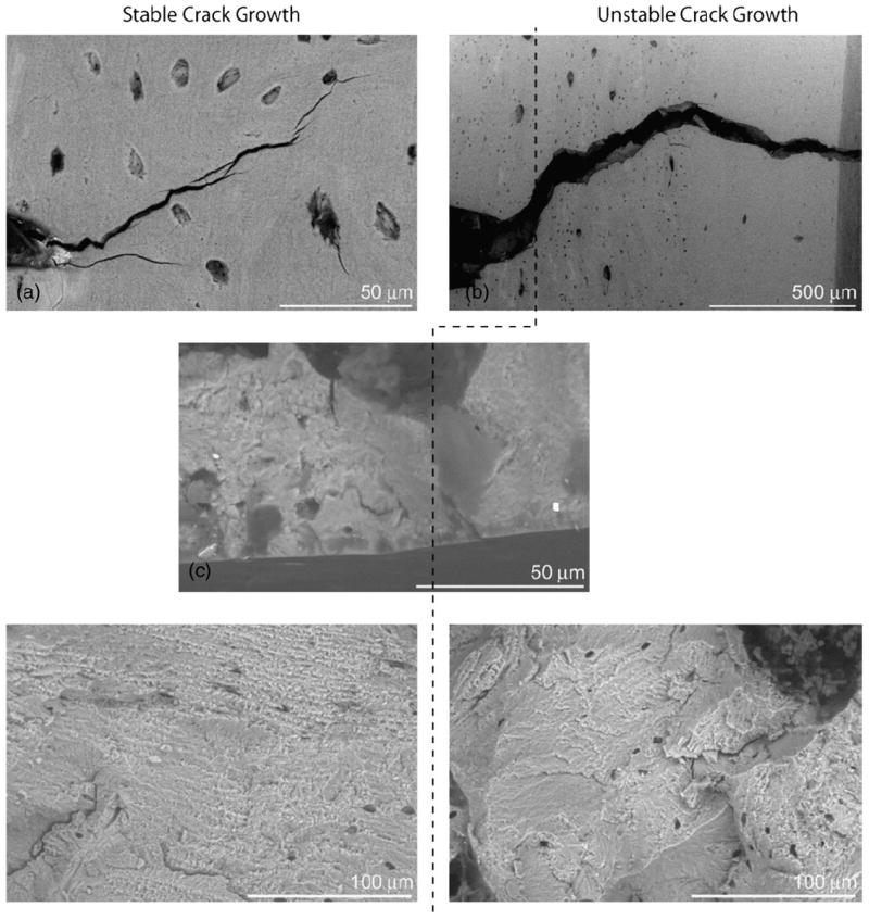
Environmental SEM images of the stable and unstable crack profiles and fractography for rat bone. The samples were tested in situ in an environmental SEM (at 35 Pa) to determine if the onset of unstable crack growth could be identified using fractography. Images (a) and (b) are of the same crack immediately before and after the onset of unstable fracture, respectively. To the left of the dotted line the crack growthwas stable and to the right of the dotted line the crack growth was unstable. It was verified via these experiments that the regions of stable and unstable crack propagation could be identified using fractography.

The “positions” of these various measurement points are shown schematically in Fig. 6 which illustrates a load–displacement curve for a notched femur. In all three cases, the fracture toughness can be calculated from:

$$K_{\mathrm{c}}=F_{\mathrm{b}}\frac{P_{\mathrm{s}}S{R}_{\mathrm{o}}}{\pi \left(R_{\mathrm{o}}^4-R_{\mathrm{i}}^4\right)}\sqrt{\pi {\Theta }_{\mathrm{c}},}$$ (9)

where P_c=P_Q and Θ_c=Θ_init for the crack-initiation method, P_c=P_max and Θ_c=Θ_init for the maximum load method, and P_c=P_f and Θ_c=Θ_inst for the instability method.¹¹ This K-solution of Eq. (9) has a claimed accuracy of “a few %” for half-crack angles between 0 and 110° [49].

Fig. 6.

Representative load-displacement curve for a sharply-notched bend specimen. On the plot are the constructions for the determination of the loads P_Q, P_max, and P_f used to compute the fracture toughness K_c. P_Q is given by the intersection of the loading curve with a line that has a 5% lower slope than the elastic deformation slope (5% secant construction), P_max is given by the maximum load, and P_f is given by the load at unstable fracture (instability). The loads are used with Eq. (9) to calculate the crack-initiation, maximum load, and fracture instability toughnesses, respectively.

The crack-initiation method will yield the lowest values, representing an intrinsic (no crack growth) toughness; this will be between 2 to 3 MPa√m for most types of bone, irrespective of orientation. The other two measures include some contribution from crack growth, which is where bone primarily derives its toughness [7,29]. As the maximum load procedure generally involves a higher load but a smaller crack size than instability, the difference in toughness values calculated using these two procedures will not be large; however, because the instability method uses a fracture load which corresponds directly to a known crack length, we believe that this approach provides a more appropriate and reliable measure of the single-valued K_c fracture toughness; additionally it incorporates contributions from both crack initiation and crack growth.

Advanced measurements

More elaborate procedures for evaluating the toughness of mouse and rat femurs involve full R-curve measurements, which fully quantify the role of crack-growth toughness, and J_c fracture toughness measurements, which incorporate the contribution from plastic deformation; in the latter case, K_c values can be back-calculated by noting that K_c,eq=(J_cE’)^1/2. In principle, both measurements require accurate monitoring of crack extension and load-line displacement, which for small samples is best done with an in situ mechanical testing stage inside an environmental SEM (see ref. [28]); however, this may not be deemed to be a reasonable proposition for routine testing.¹²

J_c fracture toughness measurements can be made through using the same definitions of fracture criticality as used above for the K_c measurements, in terms of the initial and final crack sizes. Although relationships for J are far less common than for K, one nonlinear-elastic solution of relevance to bone is the edge-cracked cylindrical pipe solution, which was originally derived for nuclear piping industry [51]:

$$J_{\mathrm{pl}}=\alpha {\sigma }_{\mathrm{o}}{\epsilon }_{\mathrm{o}}\pi R_{\mathrm{m}}{\left(1-\frac{\Theta }{\pi }\right)}^2{h}_1{\left(\frac{M}{M_0}\right)}^{n+1},$$ (10)

where α, σ_o, ε_o, and n are determined from fitting the stress–strain curve to the Ramberg–Osgood constitutive relationship: ε/ε_o=σ/σ_o + α(σ/σ_o)ⁿ. M₀ is given by:

$$M_0=4{\sigma }_{\mathrm{o}}{R}_{\mathrm{m}}^{2}t\left[\cos \left(\frac{\Theta }{2}\right)+0.5\sin \left(\frac{\Theta }{2}\right)\right],$$ (11)

and h₁ is the plastic geometric factor determined from tabulated values in ref. [51]. This solution is valid for 0.5>Θ/π>0 and for 20≥R_m/t≥5 [51]. Eq. (10) defines the plastic component of J, whereas the elastic component is K²/E′, as described above; the total J is then the sum of these two components. This solution, however, is only valid for nominally thin-walled cylinders, specifically for R_m/t≥5, which limits its strict applicability to bones, in particular mouse and rat femurs which tend to be more akin to thick-walled cylinders with R_m/t typically varying from 2 to 4. Currey has tabulated common values of R_m/t for a variety of animals and found that this ratio ranges from 1 to 4 for most land mammals; R_m/t only exceeds 5 for certain species of birds [52]. Unfortunately, the accuracy of the J-solution in Eq. (10) is not known for values of R_m/t<5.

Evaluation of toughness testing methods

To examine the use of some of these toughness measurement techniques for small animal bone testing and in particular to deduce the expected variation in measured values, a series of large-N studies was performed on mouse and rat bone. Specifically, femurs from 28 wild-type rats (14 tested in the notched condition and 14 in the unnotched condition) and 15 wild-type mice (all tested notched) were evaluated in:

• unnotched three-point bending — to measure the work to fracture, W_f,

• notched three-point bending — to measure the single-value fracture toughness, both under linear-elastic, K_c (Eq. (9)) and nonlinear-elastic, J_c (Eq. (10)) conditions,

• for comparison of the coefficients of variation (CV), measurements of the elastic (bending) modulus E (Eq. (12)) and yield and ultimate tensile strength, σ_y, σ_u, (Eq. (13)) were also made on unnotched rat femurs.¹³

Methods

Preparation

15 mouse femurs were collected from C7BL/6J mice (all male), sacrificed at age 154 days, the soft tissue removed, and the whole bones frozen in HBSS-soaked gauze at −20 °C. 28 rat femurs from Sprague Dawley rats (all female) were similarly collected from rats sacrificed at an age of 180 days, the soft tissue removed, and the whole bones was stored in 70% ethanol at 20 °C. Prior to testing, the ends of each bone were cut off using a low-speed saw to accommodate full bending of the femur without contacting the loading apparatus (Fig. 3). The mouse bones were ~15 mm long, with a mean cortical wall thickness t of 0.19 mm (S.D.=0.01 mm) and mean outer radius R_o of 0.82 mm (S.D.=0.02 mm); corresponding rat bones were ~35 mm long, with a mean cortical thickness t of 0.67 mm (S.D.=0.06 mm) and mean radius R_m of 1.75 mm (S.D.=0.07 mm). R_m/t values ranged from 2.6 to 3.8 in mouse bone and from 1.8 to 2.7 in rat bone.

Notched three-point bend testing

For the rat femurs, a low-speed saw was used to start a notch in the mid-femur region; mouse femurs did not require this step since they have much thinner walls. As noted above, notches were cut into the mid-shaft region using standard razor blades irrigated with 1 μm diamond suspension to generate a sharp starter notch. The notch was cut into the posterior of the bone, mid-shaft, such that the bone could lay with the notch facing down in the on the outer span of the three-point-bend rig.

After notching, each femur was immersed in HBSS for 24 h and heated to 37 °C by immersion in a water bath for 1 h prior to testing. The mouse femurs were tested in three-point bending on an EnduraTec Elf 3200 mechanical testing machine (BOSE, Eden Prairie, MN) with a outer loading span of S=4.7 mm. The rat femurs were tested in three-point bending on an MTS 831 (MTS Systems Corporation, Eden Prairie, MN) with a outer span of S=10.3 mm. Each femur was placed such that the posterior surface was resting on the lower supports and the notch opposite of the middle loading pin (this allowed for the posterior surface to be in tension with the anterior surface in compression). The notched mouse and rat femurs were tested with a displacement rate of 0.001 mm/s until failure.

Following testing, samples were examined in an SEM (Hitachi S-4300SE/N ESEM, Hitachi America, Pleasanton, CA), and the dimensions and the initial and instability half-crack angles were measured directly. Fracture toughness K_c values were computed using Eq. (9), employing the three methods of defining fracture criticality: crack initiation, maximum load and crack instability, as described above. Corresponding nonlinear-elastic J measurements were made from the same experiments using Eq. (10) for the J-solution for an edge-cracked cylinder in bending. Electronic calipers were used to measure the dimensions of the unnotched rat femurs.

Although variations in displacement rate of testing were not part of this study, they can influence measurements of the fracture toughness of bone [43]. However, it takes many orders of magnitude change in strain or displacement rate to have any significant effect on the toughness. For example, Zioupos [43] reported a increase in the K_c value for equine hoof walls by ~30% for a five orders of magnitude increase in testing displacement rate [43]. In the literature displacement rates for testing bone are typically between 0.0004 and 0.08 mm/s although larger variations have been examined [21,24,25]. In this study, we used a displacement rate of 0.001 mm/s, which is in the middle of this range and provided excellent reproducibility.

Other mechanical property measurements

14 rat femurs (N=14) were tested in similar fashion, immersed in HBSS for 24 h and heated to 37 °C prior to testing, only in the unnotched condition in order to measure the elastic modulus E, yield σ_y and ultimate tensile σ_u strengths and work to fracture, W_f. The unnotched rat femurs were tested with a displacement rate¹⁴ of 0.01mm/s until failure. Work to fracture values were calculated by measuring the area under the load/load-point displacement curve and dividing by twice the area of the fracture surface, as measured in the SEM. Bending modulus and strength parameters were calculated using the relations given in ref. [13]; specifically:

$$E=\frac{T{S}^3}{48I},$$ (12)

$${\sigma }_{\mathrm{y}}=\frac{P_{\mathrm{y}}S{r}_{\mathrm{m}}}{4I},{\sigma }_{\mathrm{u}}=\frac{P_{\max }S{r}_{\mathrm{m}}}{4I},$$ (13)

where T is the slope of the load/load-point displacement plot, I is the second moment of inertia for femoral cross section, and P_y and P_max are, respectively, the yield load (at the onset of nonlinearity in the load/displacement plot) and the maximum load.

Analysis of mechanical property results and their variability

Mechanical property data (work to fracture, bending modulus and strength parameters) for the rat (N=14) and mouse (N=15) femur bones are listed in Table 1. First, we discuss the observed variability of these bone toughness measurements in relation to that of strength and stiffness. Then, we consider in greater detail the best ways to measure the toughness of small animal bone and the likely variation in results associated with the various methodologies used.

Table 1.

Mechanical property results and their respective coefficients of variation for rat (N=14) and mouse (N=15) femurs

Mechanical property	Units	Average	Standard deviation	Coefficient of variation
Rat femurs (N=14)
Bending modulus	E (GPa)	3.44	0.68	0.20
Yield stress	σy (MPa)	87.77	15.17	0.17
Ultimate tensile stress	σu (MPa)	158.32	22.94	0.15
Work to fracture	Wf (kJ/m2)	4.90	1.08	0.22
Fracture toughness
Crack initiation*	Kc (MPa√m)	2.16	0.67	0.31
Maximum load		3.63	0.43	0.12
Crack instability		4.89	0.93	0.19
Mouse femurs (N = 15)
Fracture toughness
Crack initiation*	Kc (MPa√m)	2.89	0.34	0.12
Maximum load		3.60	0.33	0.09
Crack instability		4.60	0.58	0.13

^*These values are strictly invalid as P_max/P_Q≥1.1.

Comparison of mechanical properties of rat bone

For the rat bone, the toughness data (normalized by the mean of the applicable data set and derived from the fracture instability method only) are presented with the modulus and yield and ultimate tensile strength results as “box and whisker” plots in Fig. 7. Corresponding coefficients of variation are compared in Fig. 8 and a statistical comparison of values is given in Appendix II.

Fig. 7.

Comparison of variation in the various mechanical properties measured for rat femurs. Each property has been normalized by the mean value of that property. The legend in the top right corner indicates the values represented by the box plots. The upper asterisk is the maximum data point, the whisker is +1 standard deviation (SD) above mean, the top of the box is quartile 3, the middle line is the median, the small box in the center is the mean, the bottom of the box is quartile 1, the lower whisker is −1 standard deviation below mean, and the lower asterisk is the minimum data point.

Fig. 8.

Comparison of the coefficient of variation (standard deviation/mean) of the various mechanical properties measured on rat femurs. In this comparison, the K_c toughness values are for the fracture instability method.

The important result from Table 1 is that, with the crack-initiation K_c values excluded (see discussion below), measurements of the toughness of bone for a single vertebrate using the fracture toughness K_c parameter have a coefficient of variation (CV) of less than 20%; this compares with a CV of ~22% for measurements of the work to fracture. Such an inherent variability in measured bone toughness values is comparable with measurements of the bending modulus, where CV ~20%, and similar to that for the bone strength where CV ~17 and 15% for the yield and ultimate tensile strengths, respectively. A statistical comparison of values is given in Appendix II.

Fracture toughness K_c values

The present fracture toughness results indicate that the toughness of mouse and rat femurs is quite similar. Fracture toughness K_c values range from 2.2 MPa√m at crack initiation to 4.9 MPa√m at fracture instability in rat femurs, compared to corresponding K_c values of 2.9 MPa√m and 4.6 MPa√m, respectively, in mouse femurs. The specific K_c values for rat and mouse bone, computed using the initiation, maximum load and instability methods and listed in Table 1, are presented in normalized form as “box and whisker” plots in Fig. 9. The corresponding coefficients of variation of the various K_c measurement techniques for rat and mouse femurs are compared in Fig. 10.

Fig. 9.

Comparison of variation in fracture toughness for the various tests performed on rat and mouse femurs. Each data set was normalized by its mean. The maximum load method for measurements on both wild-type rat and mouse femurs shows the least variation.

Fig. 10.

Comparison of coefficients of variation (standard deviation/mean) for the various fracture toughness measurements in rat and mouse bone.

Examination of these data indicates, as expected, that the fracture toughness measured using the crack-initiation method gives the lowest values whereas the toughness values measured using the maximum load and instability methods are comparable. The variability of the crack-initiation toughness is very high, however, with CVs of over 30% for the rat femurs. We believe that this is because the 5% secant construction used to estimate the point of crack initiation is particularly inaccurate in rat bones due to the extent of plasticity compared to small section sizes (which also affects the compliance); this is evident by the fact that P_max/P_Q ratios all exceed 1.1, making these measurements strictly invalid according to the ASTM standard [18]. Because the 5% secant construction is clearly not an accurate measure of a fixed extent of crack extension (which should be 2% of the remaining uncracked ligament), we do not recommend the crack-initiation method for determining the K_c fracture toughness of small animal bones.

However, it should be noted that K_c toughness values determined by all three methods are at the limit of validity according to ASTM Standards [18]. In the present study, estimated plastic-zone sizes between crack initiation and fracture instability range from roughly 100 to 450 μm¹⁵; these need to be roughly an order of magnitude smaller than the diameter of the bone for small-scale yielding conditions to apply, i.e., to ensure K-dominance at the crack tip. Whereas this is essentially met in the rat femurs, in mouse femurs it is strictly only met for stress intensities up to 3.0 MPa√m. However, as the ASTM small-scale yielding criterion [18] tends to be rather conservative, we believe that a stress-intensity characterization is appropriate for both types of small animal femurs. Plastic-zone sizes also need to be small compared to the sample thickness for plane-strain conditions to apply. For rat and mouse bone, this implies that the thickness of the cortical shell is an order of magnitude larger than the maximum size of the plastic zone. As this is clearly not met in either the rat or mouse bone femurs, measured K_c toughnesses must be considered as plane-stress (or more strictly non-plane-strain) values. As the reality is the whole bone, which is the entity being tested, there is nothing inherently wrong with this; however, in studies where bones of widely varying sizes are evaluated, since plane-strain conditions do not prevail,¹⁶ it is possible that the actual measured toughness values may be slightly affected by the physical size of the bone, i.e., larger bones may show slightly lower toughness values as the prevailing stress-state would be closer to a plane-strain condition.

Thus, K_c toughness values, determined for mouse and rat femurs, can be considered as valid “plane-stress” measurements. As noted above, whether computed at maximum load or at fracture instability, the coefficients of variance for such K_c measurements are all below 20% (Fig. 10). Although not as simple to perform, the definition of the K_c value at fracture instability is preferred to a measurement at maximum load, because it more accurately identifies specific applied loads and crack sizes at the onset of unstable fracture.

Fracture toughness J_c values

Corresponding nonlinear-elastic estimates of the toughness of the rat and mouse femurs, in terms of J_c values, are listed in Table 2, together with approximate (back-calculated) equivalent stress-intensity values, K_c,eq=(J_cE′)^1/2. As with the LEFM measurements, the toughness was calculated at maximum load and at fracture instability, although the latter instability measurements could not be made for the rat femurs as the half-crack angles after subcritical crack growth were too large and well beyond the validity of Eq. (10). In any event, this J-solution is strictly only valid for R_m/t values greater than 5, whereas values of R_m/t ranged from a low of 1.8 in rat bone to a high of 3.8 in mouse bone. Since Eq. (10) is to our knowledge is the only J-solution presently available solution for edge-cracked cylindrical pipes applicable to such small animal bone structures, and the accuracy of the solution is uncertain for R_m/t values less than 5, we do not recommend the J-approach for the toughness evaluation of small animal bones at this time. We include the results though, as the computed J_c values do yield an estimate of the contribution to the overall toughness from plastic deformation in the bone.

Table 2.

Nonlinear-elastic J_c values of the fracture toughness, and equivalent (back-calculated) K_c,eq values, for rat (N=14) and mouse femurs (N=15) and their respective coefficients of variation

Mechanical property	Units	Average	Standard deviation	Coefficient of variation
Rat femurs (N =14)
J-integral
Maximum loada	Jc (kJ/m2)	15.90	8.17	0.51
Crack instabilityb		–	–	–
Effective fracture toughness
Maximum load	Kc,eq (MPa√m)	7.18	1.85	0.26
Crack instabilityb		–	–	–
Mouse femurs (N = 15)
J-integral
Maximum loadc	Jc (kJ/m2)	10.68	3.05	0.29
Crack instabilityd		26.71	14.12	0.53
Effective fracture toughness
Maximum load	Kc,eq (MPa√m)	7.85	1.33	0.17
Crack instability		12.28	2.96	0.24

^aValidity achieved when a, b>25 J/σ_f>3.2 mm.

^bNo value could be calculated as J-solution is invalid as Θ/π≫0.5.

^cValidity achieved when a, b>25 J/σ_f>2.3 mm.

^dValidity achieved when a, b>25 J/σ_f>5.3 mm.

As noted above, computed nonlinear-elastic toughness J_c values for the rat and mouse femurs are listed in Table 2, together with the back-calculated K_c,eq values. Comparison of the latter values with the linear-elastic K_c values in Table 1 indicates that the J-approach does elevate the K_c toughness by a factor of roughly 2 to almost 3 in the rat and mouse bone, respectively, in essence by including the contribution to the toughness from plastic (inelastic) deformation and mixed-mode loading.

The strict validity of the measured J values is determined by the uncracked ligament exceeding 25 J/σ_f, the latter being on the order of 3 mm for the rat bone and ~2–5 mm for the mouse bone. This implies that the J-field is barely valid for rat femurs, and well beyond validity for mouse femurs; furthermore, as plane-strain conditions are not met, calculated J_c values reflect a plane-stress fracture toughness. For the former reason, we do not recommend such J-based toughness measurements for small animal bone testing.

Comparative variability of toughness measurements

Finally, it is pertinent to compare these coefficients of variation with studies on the mechanical properties of bone taken from a large range of mammalian species, e.g., provided in the survey of Currey et al. [36]. Our measured CVs of less than 20% for (maximum load and fracture instability) K_c values are lower than that for the toughness measurements reported in the study of Currey et al., where the CVs ranged from 28 to 46% for unnotched toughness tests such as the work to fracture. (Note that we found a higher CV, of 22%, for the W_f measurements on rat bone in the current study). For this reason, we believe that fracture mechanics based measurements are far more reliable for evaluating the toughness of small animal bone, as compared to determining the energy, e.g., the work to fracture, to break unnotched samples. Both types of toughness measurements are useful, however.

Nonlinear-elastic fracture mechanics, e.g., the J-integral method, is in many respects an ideal means of characterizing toughness of bone as it incorporates the contribution from plasticity and characterizes single-mode and mixed-mode driving forces for crack propagation in bone. Although in the present work, there was a larger variation in the results obtained with this technique, we believe that this arose from the fact that Eqs. (10)-(11) were derived for thin-walled cylinders (with uniform circular cross sections and radii at least five times larger than the wall thicknesses). This, however, should not reflect any inadequacies of the use of nonlinear-elastic fracture mechanics to study other geometries.

Discussion

There are a variety of choices when selecting mechanical test methods to evaluate the fracture resistance of bone subjected to various biological factors such as aging, disease and therapeutic treatments. As many of the studies of these biological factors have used small animal models, the specific application of the test methods to small mammalian bones has been the primary focus of this review.

These test methods can generally be classed into two major categories, namely unnotched (e.g., the work to fracture) and notched/precracked (e.g., fracture mechanics based methods) techniques. Although the fracture mechanics methodology is more recent and certainly can be more sophisticated, for the assessment of bone fragility, both approaches can offer useful information. As discussed above, in bone, unnotched toughness tests such as the work to fracture assess both the role of the inherent bone-matrix structure (or architecture) and the presence of pre-existing defects in influencing the applied loading conditions to cause fracture; in this regard they are essentially equivalent to strength measurements (strength can be obtained in the same tests simultaneously with work to fracture). Since the size and internal distributions of such pre-existing flaws would not necessarily be known, we cannot define which flaw led to the failure; moreover, the effect of such pre-existing flaws on the toughness of bone cannot be distinguished from any fundamental changes in the bone-matrix structure. Accordingly, fracture mechanics procedures avoid this ambiguity of an unknown distribution of flaws through the use of a worst-case flaw, achieved through the creation of a precrack or sharpened notch; the measured toughness can then be associated solely with the inherent ability of the bone-matrix structure to resist fracture. However, such methods might not necessarily be as sensitive as unnotched methods to bone containing a higher fraction of microcracks, associated for example with aging or fatigue damage. For this reason, we believe that fracture mechanics measurements should be combined with traditional strength measurements to offer the optimum solution for evaluating the fracture properties of bone.

This paper has discussed the fracture mechanics measurements that can be applied to bone; namely, crack-initiation, maximum load, and instability methods. The crack-initiation method is considered the least useful of these methods as it does not take into account the amount of stable-crack growth that occurs in bone prior to outright fracture. The difference between the maximum load and instability methods is that the former uses a combination of the maximum load and initial half-crack angle and the latter uses a combination of the load and the half-crack angle at the onset of unstable fracture. Although the instability method is more difficult to apply and the coefficient of variation was higher than the maximum load method, it is still the preferred measure of the toughness of small animal bones. The instability method is superior to the other methods because it combines the real crack size and load when calculating the driving force for fracture. This represents a truer depiction of the toughness of small animal bones.

The question that now arises though is which of the fracture mechanics methods is most appropriate for bone, and specifically for the evaluating the changes in the bone toughness due to biological changes, etc., in small animal studies. Where relatively large-sized specimens (i.e., tens of millimeters or more in size) can be used, i.e., to evaluate the toughness of cortical bone in larger mammals such as humans, it is our opinion that a preferable approach is to utilize both a nonlinear-elastic fracture mechanics methodology (e.g., involving J measurements),¹⁷ in order to incorporate the important contribution from plasticity to the overall toughness, together with resistance-curve measurements to incorporate the toughness associated with crack growth (as this is where bone primarily derives its fracture resistance) [28]. These methods are recommended based on the previous work of ourselves and others [6,7,28], and the fact, which has been emphasized throughout the present work, that bone exhibits stable crack growth prior to failure and R-curve analysis is the comprehensive means of capturing this behavior (Fig. 2). However, for such tests on whole bone from small animal studies, these procedures are complicated and due to the small dimensions of the bone, may not even be feasible. Accordingly, in this work we have tried to demonstrate the utility of using whole bone fracture toughness testing on femurs as an effective means of assessing bone fragility for small animal studies. Although nonlinear-elastic J measurements would normally be preferred, existing J-solutions are not always applicable for small animal bones; indeed, they are not expected to be applicable for the whole bone testing of most land mammals [52], as in the present case of rat and mouse femurs where the resulting J_c toughness values were mostly invalid. Furthermore, the experiments to measure J_c can be difficult to perform, especially for very large N studies. Consequently, we recommend the use of K_c fracture toughness measurements, where fracture is defined at the fracture instability point, i.e., not at crack initiation but rather when the crack propagates unstably. This represents an appropriate plane-stress measurement, which is still relatively straightforward to perform, although it does require some degree of high-resolution imaging, e.g., in the SEM, to determine the extent of subcritical cracking prior to final failure. In addition to its relative simplicity, the advantage of this procedure is that by incorporating the occurrence of subcritical cracking in the toughness calculation, the vital contribution of the crack-growth toughness in the value of K_c is included; its disadvantage is that the contribution from plasticity will be naturally less than in equivalent J_c measurements. However, our studies show that careful sample preparation together with precise definition of the loads and crack sizes at fracture instability can lead to fracture toughness measurements with coefficients of variation under 20% in small animal bone testing. This represents a significant improvement over the work to fracture measurements where the variability is generally significantly larger [36].

This variability is extremely important to take into consideration when designing medical studies to investigate the influence of biological factors on the mechanical properties of bone. This work has examined a range of mechanical properties with a sample population that is larger than that often used in these studies. Commonly in small animal studies that examine the influence of different biological factors, the number of samples for each group ranges from 6–13 [54-61]. The results of this study can be used to then estimate what magnitude of differences can be detected at a statistically significant level for these properties. To compare the means of two populations with equal variance, the t-test can be used, as given by:

$$\mathrm{t}=\frac{{\zeta }_1-{\zeta }_2}{\mathrm{SD}\sqrt{\frac{1}{{\mathrm{N}}_1}+\frac{1}{{\mathrm{N}}_2}}},$$ (14)

where ζ₁ and ζ₂ are the means of the two populations, SD is the standard deviation, and N₁ and N₂ are the number of samples for each population. Rearranging this equation:

$${\zeta }_1-{\zeta }_2=\mathrm{t}\left(\mathrm{SD}\sqrt{\frac{1}{N_1}+\frac{1}{N_2}}\right),$$ (15)

allows the calculation of the difference in means that will be statistically significant at the P<0.05 level for the rats and mice having standard deviations in properties the same as found in this study. These differences for N₁=N₂=6 and N₁=N₂=13 are shown in Table 3.

Table 3.

Differences in means that are expected to be statistically significant at the P<0.05 level for the mechanical properties examined in this study.

Mechanical property	Units	Difference for N1=N2=6	Difference for N1=N2=13
Rat femurs (N =14)
Bending modulus	E (GPa)	0.7	0.5
Yield stress	σy (MPa)	15.9	10.2
Ultimate tensile stress	σu (MPa)	24.0	15.4
Work to fracture	Wf (kJ/m2)	1.1	0.7
Fracture toughness
Crack initiation	Kc (MPa√m)	0.7	0.5
Maximum load		0.5	0.3
Crack instability		1.0	0.6
Mouse femurs (N= 14)
Fracture toughness
Crack initiation	Kc (MPa√m)	0.4	0.2
Maximum load		0.4	0.2
Crack instability		0.6	0.4

The approach recommended here is to utilize instability-based K_c measurements because the observed variability is much lower, as described in Appendix II. We believe that this represents a significant improvement over work to fracture measurements as not only does the animal population have a natural variation, but the test method chosen for the study also has inherent variability which can be larger than the variation observed in the samples of the test. Statistical calculations such as ANOVA and t-tests may not be sufficient in these cases to determine significance. It is important to acknowledge that the results of a study must be more robust to overcome the variability introduced by the testing method. For fracture evaluation in small animal bone, this study has shown that any such observed variation in the fracture toughness of the bone samples must be in excess of 20% for meaningful conclusions to be made.

Conclusions

The methodologies available to measure the toughness (fracture resistance) of small mammalian bone have been evaluated quantitatively. Test procedures evaluated include the work to fracture W_f, the linear-elastic fracture mechanics based fracture toughness K_c and the nonlinear-elastic fracture mechanics based J_c toughness. We make a distinction between W_f, which uses an unnotched test procedure as compared to the fracture mechanics methods which employ notched/precracked samples. The expected variation for each of these tests was quantified by performing a large-N study with wild-type rats and mice.

It is concluded that for small animal studies, linear-elastic fracture mechanics techniques to determine a plane-stress K_c value provide the best compromise of ease of measurement and accuracy, with worst-case accuracy in K_c measurement estimated at better than 17%. Procedures to evaluate the value of K_c specifically at maximum load or preferably at fracture instability are recommended. For both wild-type mouse and rat femurs, a coefficient of variation (standard deviation/mean) of less than 20% was found for K_c toughness measurements, which compares well with the expected variability in similar measurements of bone modulus and bone strength. The coefficient of variation was significantly higher for the work to fracture measurements; use of this test would result in having less statistical power to discern toughness changes between treatment groups in, for example, a drug trial.

Nomenclature

a

crack length

a_c

critical crack size

a_init,a_inst

crack size at crack initiation, fracture instability

A_pl

area under the load/plastic load–point displacement curve

b

uncracked ligament (W – a)

B

specimen thickness

C

compliance

CV

coefficient of variation (standard deviation/mean)

c

distance from the neutral axis

E, E′

Young’s modulus

F_b

geometrical factor in K_I solution for an edge-cracked cylindrical pipe

f_ij (θ), f_ij(θ,n)

angular functions of θ and n

G

strain-energy release rate

G_c

critical value of strain-energy release rate

I

second moment of inertia

I_n

integration constant in the HRR singular field

K

linear-elastic stress-intensity factor

K_c, K_Ic

critical values of stress intensity – fracture toughness

K_c,eq

equivalent value of K_c, back-calculated from J measurements

K_I, K_II, K_III

stress-intensity factors in modes I, II, III

J

J-integral

J_c, J_Ic

critical values of J-integral – fracture toughness

M

bending moment

n

strain hardening coefficient

N

number of samples

P

applied load

P_c

critical load at fracture

P_f

critical load at fracture instability

P_max

maximum load

P_y

yield load (at the onset of nonlinearity in load/load-line displacement plot)

Q, f(a/W), f_b

geometry factors in the definition of K

R_m, R_i, R_o

mean, inner and outer radius of the cortical shell

r

radial distance ahead of a crack tip

r_y

plastic-zone size

S

outer loading span in three-point bending

SD

standard deviation

T

slope of load/load-point displacement curve

t

mean wall (cortex) thickness

W

specimen width

W_f

work to fracture (energy per unit area)

α

constant in Ramberg–Osgood relation

Δa

stable crack extension

ε

strain

η

geometry factor in J-solution

μ

shear modulus

ν

Poisson’s ratio

Θ

half-crack angle

Θ_init, Θ_inst

half-crack angle at crack initiation, fracture instability

σ

stress

σ_app

applied stress

σ_b

applied bending stress

σ_f

flow stress (mean of yield and ultimate tensile strengths)

σ_ij

local stresses

σ_o, ε_o

reference stress and strain in Ramberg–Osgood relation

σ_u

ultimate tensile strength

σ_y

yield strength

ζ₁, ζ₂

population means

Appendix I. Estimation of worst-case errors in computing stress intensities (Eqs. (5)-(9))

There are potential sources of error in the determination of stress intensities from the edge-cracked thick-walled cylinder in bending stress-intensity solutions (Eqs. (5)-(9)) due to (i) the experimental precision with which the bone geometry and mechanical parameters can be measured and (ii) the deviations of the cross sections of rat and mouse bone from the circular cylinder with uniform wall thickness which is assumed for the K-solution.

1. Consideration of Eqs. (5)-(9)) used to calculate the stress intensity in a thick-walled pipe reveals that, of the geometric parameters, uncertainties in the radius have the greatest effect on the accuracy of the solution. For rat and mouse bones, the following measurement uncertainties were estimated based on the precision of the measuring calipers and by comparison to SEM images: radius (mean radius of the bone), 0.3% (0.01 mm); thickness (mean wall thickness), 1.4% (0.01 mm), crack angle 1.7% (3°); span (0.5% (0.05 mm). When combined with the 0.3% (0.1 N) uncertainty expected from the load cell, a propagation of errors analysis yields an estimated uncertainty in the measured stress intensity of ~4%.

2. The uncertainty obtained above is due to measurement variability in the experimental parameters for a circular cylinder with a uniform wall thickness; however, the cross section of mouse and rat femurs is neither perfectly circular nor of uniform wall thickness, as depicted in Fig. A1, which gives rise to a further source of error in the computed stress intensity. These errors arise from the calculation of the difference between the outer and the inner radius (ΔR=R_o−R_i) used in the stress term of the K-solution and in the determination of the average thickness, t, of the cortex. The errors in ΔR and t are given by:

   $$\mathrm{\delta \Delta }R=\frac{1}{2}\left[\frac{\left(\mathrm{\Delta }{R}_{\max }-\mathrm{\Delta }{R}_{\mathrm{avg}}\right)+\left(\mathrm{\Delta }{R}_{\mathrm{avg}}-\mathrm{\Delta }{R}_{\min }\right)}{2}\right],$$ (A1)

   and for t:

   $$\delta \mathrm{\Delta }t=\frac{1}{2}\left[\frac{\left(t_{\max }-t_{\mathrm{avg}}\right)+\left(t_{\mathrm{avg}}-t_{\min }\right)}{2}\right],$$ (A2)

   where ΔR_avg is given by:

   $$\mathrm{\Delta }{R}_{\mathrm{avg}}=\frac{\left(R_{\mathrm{o},\max }-R_{\mathrm{o},\min }\right)}{2}-\frac{\left(R_{\mathrm{i},\max }-R_{\mathrm{i},\min }\right)}{2},$$ (A3)

   and R_o,max, R_o,min, R_i,max, and R_i,min are the maximum outer radius, minimum outer radius, maximum inner radius, and minimum inner radius, respectively (see Fig. A1). Based on experimentalmeasurements of the dimensions of the bone, the deviations of the cross section from circular and uniform wall thickness result in errors of 5% in ΔR and 7% in t. This leads to an uncertainty in the stress intensity of 17%, which is clearly much larger than that due to measurement uncertainties.

Fig. A1.

Schematic diagrams of the locations where the radii and thicknesses were measured on the fracture surface of the rat bone. The cross section is not circular nor has a uniform wall thickness (i.e., R_min≠R_max and t_min≠t_max.). The measurement locations for the two-point average for the radius and the six-point average for the thickness are indicated.

We used a two-point average to measure the radius and a six-point average to measure the cortical thickness. The two-point average was chosen for the radius because it is unambiguous to define and is not subject to bias by the observer (in this study, values obtained by the two methods differed only by 1–5%). However, we recommend an average of six evenly spaced measurements of the unnotched region for measuring the thickness (Fig. A1). This method was chosen to minimize effects due to inhomogeneities in the thickness of the cortex. In contrast, we found that a two-point average of the thickness could lead to increased errors because the extent of the maximum and minimum thickness regions can be relatively small and thus not typical of the average cortex thickness.

Appendix II. Statistical comparisons of the variations of the mechanical tests

Parametric (mean ξ, standard deviation s) and non-parametric (median, quartiles) statistics were computed for each group of mechanical measurements. To compare standard deviations between groups, the F statistic $s_1^2/s_2^2$ was calculated and tested for significance (the standard deviations used in this test were normalized to the mean of each group). A P value <0.05 was considered significant; we also note marginal significance at 0.05<P<0.1.

1. Two-sided F tests between the three different fracture toughness measurement techniques for both the rat and mouse datasets are summarized in Table A1. In mice, the fracture instability methods has significantly smaller variances compared to the crack-initiation method (instability was marginally significant). The maximum load variance was smaller than the instability variance, but this difference was not significant. The maximum load and instability tests in mice retained valid half-crack angles for each sample.

   Table A1.

   F ratios $(s_1^2/s_2^2)$ between the different toughness evaluation methods. The comparison is ordered with the group with the larger standard deviation listed first

   Test comparison	F-ratio
   Rats: Kc, initiation vs. Kc, max load	2.41
   Rats: Kc, instability vs. Kc, max load	4.66*
   Rats: Kc, instability vs. Kc, initiation	1.94
   Mice: Kc, initiation vs. Kc, max load	1.06
   Mice: Kc, max load vs. Kc, instability	3.05**
   Mice: Kc, instability vs. Kc, initiation	2.88***

   ^*

   P<0.01.

   ^**

   P<0.05.

   ^***

   0.05<P<0.1 (marginally significant).

   In rats the variance of the maximum load method was smaller than for the initiation method but this was not significant. In contrast, the maximum load variance was significantly smaller than that of the instability method. We attribute the large variance in the instability to the fact that the half-crack angles exceeded somewhat the bounds of the K-solution in the instability test. Similar to the fracture tests in mice, the initiation method exhibited a higher variation in results than the other two methods, as noted in the text, primarily due to the inaccuracy of the 5% secant construction in the presence of local plasticity. Based on these analyses, we recommend use of the maximum load or preferably the fracture instability method, with attention to the K-solution validity with respect to the size of the half-crack angle.

2. Next, we compare the variances of the fracture toughness measurement methods to the work to fracture test (Table A2). In both groups, one of the fracture toughness methods had a significantly smaller variance compared to work to fracture and the other was marginally significant. We conclude that fracture toughness measurements have a lower variance than work to fracture measurements. While the former measurement is simpler to perform, a correctly executed fracture toughness test should have more statistical power to discern clinically significant changes in treatment groups in small mammals.

   Table A2.

   Two-sided F tests $(s_1^2/s_2^2)$ between the work to fracture and different toughness evaluation methods. The comparison is ordered with the group with the larger standard deviation listed first

   Test comparison	F-ratio
   Rats: Wf vs. Kc, initiation	2.62
   Rats: Wf vs. Kc, max load	6.31*
   Rats: Wf vs. Kc, instability	1.35
   Mice: Wf vs. Kc, initiation	10.14*
   Mice: Wf vs. Kc, max load	10.77*
   Mice: Wf vs. Kc, instability	3.53**

   ^*

   P<0.01.

   ^**

   P<0.05.

3. We compared the variance observed in this study for the work to fracture W_f to that reported by Currey et al. [36] for a large data set of cortical bone samples derived from a variety of animals (bovine, horse, human, and various vertebrates). Specifically, the CV (22%) of the work to fracture test performed in the current study on rats was compared to the CV (33.8%) observed by Currey et al. A two-sided test was performed and although the variance in the Curry et al. data set is larger than that reported here (F=2.08), the difference is not statistically significant (P>0.1). We conclude that work to fracture tests may yield lower variance if only one species is investigated but, overall, a CV of 20–30% is to be expected for this type of test.

References

- 1.Behiri JC, Bonfield W. Orientation dependence of the fracture mechanics of cortical bone. J Biomech. 1989;22:863–7. doi: 10.1016/0021-9290(89)90070-5. [DOI] [PubMed] [Google Scholar]
- 2.Kalkwarf HJ, Specker BL, Bianchi DC, Ranz J, Ho M. The effect of calcium supplementation on bone density during lactation and after weaning. New Engl J Med. 1997;337:523–8. doi: 10.1056/NEJM199708213370803. [DOI] [PubMed] [Google Scholar]
- 3.Zioupos P, Currey JD. Changes in the stiffness, strength, and toughness of human cortical bone with age. Bone. 1998;22:57–66. doi: 10.1016/s8756-3282(97)00228-7. [DOI] [PubMed] [Google Scholar]
- 4.Shane E, Addesso V, Namerow P, McMahon DJ, Lo S, Staron RB, et al. Alendronate versus calcitriol for the prevention of bone loss after cardiac transplantation. New Engl J Med. 2004;350:767–76. doi: 10.1056/NEJMoa035617. [DOI] [PubMed] [Google Scholar]
- 5.Roodman GD. Mechanisms of bone metastasis. New Engl J Med. 2004;350:1655–64. doi: 10.1056/NEJMra030831. [DOI] [PubMed] [Google Scholar]
- 6.Vashishth D. Rising crack-growth-resistance behavior in cortical bone: implications for toughness measurements. J Biomech. 2004;37:943–6. doi: 10.1016/j.jbiomech.2003.11.003. [DOI] [PubMed] [Google Scholar]
- 7.Nalla RK, Kruzic JJ, Kinney JH, Ritchie RO. Mechanistic aspects of fracture and R-curve behavior in human cortical bone. Biomaterials. 2005;26:217–31. doi: 10.1016/j.biomaterials.2004.02.017. [DOI] [PubMed] [Google Scholar]
- 8.Lane NE, Yao W, Balooch M, Nalla RK, Balooch G, Habelitz S, et al. Glucocorticoid-treated mice have localized changes in trabecular bone material properties and osteocyte lacunar size that are not observed in placebo-treated or estrogen-deficient mice. J Bone Miner Res. 2006;21:466–76. doi: 10.1359/JBMR.051103. [DOI] [PMC free article] [PubMed] [Google Scholar]
- 9.Yao W, Cheng Z, Koester KJ, Ager JW, Balooch M, Pham A, et al. The degree of bone mineralization is maintained with single intravenous bisphosphonates in aged estrogen-deficient rats and is a strong predictor of bone strength. Bone. 2007;41:804–12. doi: 10.1016/j.bone.2007.06.021. [DOI] [PMC free article] [PubMed] [Google Scholar]
- 10.Balooch G, Yao W, Ager JW, Balooch M, Nalla RK, Porter AE, et al. The aminobisphosphonate risedronate preserves localized mineral and material properties of bone in the presence of glucocorticoids. Arthritis & Rheum. 2007;56:3726–37. doi: 10.1002/art.22976. [DOI] [PMC free article] [PubMed] [Google Scholar]
- 11.Taylor D, Hazenberg JG, Lee TC. Living with cracks: damage and repair in human bone. Nature Mater. 2007;6:249–317. doi: 10.1038/nmat1866. [DOI] [PubMed] [Google Scholar]
- 12.Turner CH, Burr DB. Basic biomechanical measurements of bone: a tutorial. Bone. 1993;14:595–608. doi: 10.1016/8756-3282(93)90081-k. [DOI] [PubMed] [Google Scholar]
- 13.Akhter MP, Cullen DM, Gong G, Recker RR. Bone biomechanical properties in prostaglandin EP1 and EP2 knockout mice. Bone. 2001;29:121–5. doi: 10.1016/s8756-3282(01)00486-0. [DOI] [PubMed] [Google Scholar]
- 14.Silva MJ, Brodt MD, Fan Z, Rho JY. Nanoindentation and whole-bone bending estimates of material properties in bones from the senescence accelerated mouse samp6. J Biomech. 2004;37:1639–46. doi: 10.1016/j.jbiomech.2004.02.018. [DOI] [PubMed] [Google Scholar]
- 15.Mulder L, Koolstra JH, den Toonder JMJ, van Eijden TMGJ. Intratrabecular distribution of tissue stiffness and mineralization in developing trabecular bone. Bone. 2007;41:256–65. doi: 10.1016/j.bone.2007.04.188. [DOI] [PubMed] [Google Scholar]
- 16.Currey JD. Mechanical properties of bone tissues with greatly differing functions. J Biomech. 1979;12:313–9. doi: 10.1016/0021-9290(79)90073-3. [DOI] [PubMed] [Google Scholar]
- 17.ASTM Standard E-399. Standard test method for linear-elastic plane-strain fracture toughness KIc of metallic materials. West Conshohocken, PA: American Society for Testing and Materials; 2006. [Google Scholar]
- 18.ASTM Standard E-1820. Standard test method for measurement of fracture toughness. West Conshohocken, PA: American Society for Testing and Materials; 2006. [Google Scholar]
- 19.Wright TM, Hayes WC. Fracture mechanics parameters for compact bone — effects of density and specimen thickness. J Biomech. 1977;10:419–25. doi: 10.1016/0021-9290(77)90019-7. [DOI] [PubMed] [Google Scholar]
- 20.Behiri JC, Bonfield W. Fracture mechanics of bone — the effects of density, specimen thickness and crack velocity on longitudinal fracture. J Biomech. 1984;17:25–34. doi: 10.1016/0021-9290(84)90076-9. [DOI] [PubMed] [Google Scholar]
- 21.Norman TL, Vashishth D, Burr DB. Fracture toughness of human bone under tension. J Biomech. 1995;28:309–20. doi: 10.1016/0021-9290(94)00069-g. [DOI] [PubMed] [Google Scholar]
- 22.Yeni YN, Brown CU, Wang Z, Norman TL. The influence of bone morphology on fracture toughness of the human femur and tibia. Bone. 1997;21:453–9. doi: 10.1016/s8756-3282(97)00173-7. [DOI] [PubMed] [Google Scholar]
- 23.Yeni YN, Brown CU, Norman TL. Influence of bone composition and apparent density on fracture toughness of the human femur and tibia. Bone. 1998;22:79–84. doi: 10.1016/s8756-3282(97)00227-5. [DOI] [PubMed] [Google Scholar]
- 24.Brown CU, Yeni YN, Norman TL. Fracture toughness is dependent on bone location — a study of the femoral neck, femoral shaft, and the tibial shaft. J Biomed Mater Res. 2000;49:380–9. doi: 10.1002/(sici)1097-4636(20000305)49:3<380::aid-jbm11>3.0.co;2-w. [DOI] [PubMed] [Google Scholar]
- 25.Phelps JB, Hubbard GB, Wang X, Agrawal CM. Microstructural heterogeneity and the fracture toughness of bone. J Biomed Mater Res. 2000;51:735–41. doi: 10.1002/1097-4636(20000915)51:4<735::aid-jbm23>3.0.co;2-g. [DOI] [PubMed] [Google Scholar]
- 26.Nalla RK, Kinney JH, Ritchie RO. Mechanistic fracture criteria for the failure of human cortical bone. Nat Mater. 2003;2:164–8. doi: 10.1038/nmat832. [DOI] [PubMed] [Google Scholar]
- 27.Yan J, Mecholsky J, Clifton KB. How tough is bone? Application of elastic–plastic fracture mechanics to bone. Bone. 2007;40:479–84. doi: 10.1016/j.bone.2006.08.013. [DOI] [PubMed] [Google Scholar]
- 28.Koester KJ, Ager JW, III, Ritchie RO. How tough is cortical human bone?: In-situ measurements on realistically short cracks. Nature Mater. 2008;7 doi: 10.1038/nmat2221. org/10.1038/nmat2221. [DOI] [PubMed] [Google Scholar]
- 29.Vashishth D, Behiri JC, Bonfield W. Crack growth resistance in cortical bone: concept of microcrack toughening. J Biomech. 1997;30:763–9. doi: 10.1016/s0021-9290(97)00029-8. [DOI] [PubMed] [Google Scholar]
- 30.Malik CL, Stover SM, Martin RB, Gibeling JC. Equine cortical bone exhibits rising R-curve fracture mechanics. J Biomech. 2003;36:191–8. doi: 10.1016/s0021-9290(02)00362-7. [DOI] [PubMed] [Google Scholar]
- 31.Yang QD, Cox BN, Nalla RK, Ritchie RO. Re-evaluating the toughness of human cortical bone. Bone. 2006;38:878–87. doi: 10.1016/j.bone.2005.10.014. [DOI] [PubMed] [Google Scholar]
- 32.Yang QD, Cox BN, Nalla RK, Ritchie RO. Fracture length scales in human cortical bone: the necessity of nonlinear fracture models. Biomaterials. 2006;27:2095–113. doi: 10.1016/j.biomaterials.2005.09.040. [DOI] [PubMed] [Google Scholar]
- 33.Ural A, Vashishth D. Cohesive finite element modeling of age-related toughness loss in human cortical bone. J Biomech. 2006;39:2974–82. doi: 10.1016/j.jbiomech.2005.10.018. [DOI] [PubMed] [Google Scholar]
- 34.Norman TL, Vashishth D, Burr DB. Effect of groove on bone fracture toughness. J Biomech. 1992;25:1489–92. doi: 10.1016/0021-9290(92)90061-5. [DOI] [PubMed] [Google Scholar]
- 35.Kruzic JJ, Kuskowski SJ, Ritchie RO. Simple and accurate fracture toughness testing methods for pyrolytic cabon/graphite composites used in heart valve prostheses. J Biomed Mater Res A. 2005;74A:461–4. doi: 10.1002/jbm.a.30380. [DOI] [PubMed] [Google Scholar]
- 36.Currey JD, Pitchford JW, Baxter PD. Variablility of the mechanical properties of bone, and its evolutionary consequences. J Royal Soc Interface. 2007;4:127–35. doi: 10.1098/rsif.2006.0166. [DOI] [PMC free article] [PubMed] [Google Scholar]
- 37.Bonfield W. Advances in the fracture mechanics of cortical bone. J Biomech. 1987;20:1071–81. doi: 10.1016/0021-9290(87)90025-x. [DOI] [PubMed] [Google Scholar]
- 38.Williams JG, Ewing PD. Fracture under complex stress-the angled crack problem. Int J Fract Mech. 1972;8:441–6. [Google Scholar]
- 39.Irwin GR. Analysis of stresses and strains near the end of a crack traversing a plate. J Appl Mech. 1957;24:361–4. [Google Scholar]
- 40.Knott JF. Fundamentals of fracture mechanics. London: Butterworth & Co.; 1976. [Google Scholar]
- 41.Ritchie RO, Gilbert CJ, McNaney JM. Mechanics and mechanisms of fatigue damage and crack growth in advanced materials. Int J Solids Struct. 2000;37:311–29. [Google Scholar]
- 42.Shang JK, Ritchie RO. Crack bridging by uncracked ligaments during fatigue-crack growth in SiC-reinforced aluminum-alloy composites. Metall Trans A. 1989;20A:897–908. [Google Scholar]
- 43.Zioupos P. Recent developments in the study of failure of solid biomaterials and bone: ‘fracture’ and ‘pre-fracture’ toughness. Mater Sci Eng C. 1998;6:33–40. [Google Scholar]
- 44.Nalla RK, Kruzic JJ, Kinney JH, Ritchie RO. Effect of aging on the toughness of human cortical bone: evaluation by R-curves. Bone. 2004;35:1240–6. doi: 10.1016/j.bone.2004.07.016. [DOI] [PubMed] [Google Scholar]
- 45.Rice JR, Rosengren GF. Plane strain deformation near a crack tip in a power-law hardening material. J Mech Phys Solids. 1968;16:1–12. [Google Scholar]
- 46.Hutchinson JW. Singular behaviour at the end of a tensile crack in a hardening material. J Mech Phys Solids. 1968;16:13–31. [Google Scholar]
- 47.Rice JR. A path independent integral and the approximate analysis of strain concentration by notches and cracks. J Appl Mech. 1968;35:379–86. [Google Scholar]
- 48.Lacire MH, Chapuliot S, Marie S. Stress intensity factors of through wall cracks in plates and tubes with circumferential cracks. ASME PVP. 1999;388:13–21. [Google Scholar]
- 49.Takahashi Y. Evaluation of leak-before-break assessment methodology for pipes with a circumferential through-wall crack: Part I. Stress intensity factor and limit load solutions. Int J Pres Ves Pip. 2002;79:385–92. [Google Scholar]
- 50.Koester KJ, Ager JW, III, Ritchie RO. The effect of aging on crack-growth resistance and toughening mechanisms in human dentin. Biomaterials. 2008;29:1318–28. doi: 10.1016/j.biomaterials.2007.12.008. [DOI] [PubMed] [Google Scholar]
- 51.Zahoor A. Ductile fracture handbook, 1. Palo Alto: Electric Power Research Institute; 1989. pp. 2–9–2–16. [Google Scholar]
- 52.Currey JD. Bones. Princeton: Princeton University Press; 2002. [Google Scholar]
- 53.Robertson DM, Robertson D, Barrett CR. Fracture toughness, critical crack length and plastic zone size in bone. J Biomech. 1978;11:359–64. doi: 10.1016/0021-9290(78)90070-2. [DOI] [PubMed] [Google Scholar]
- 54.Akhter MP, Wells DJ, Short SJ, Cullen DM, Johnson ML, Haynatzki GR, et al. Bone biomechanical properties in lrp5 mutant mice. Bone. 2004;35:162–9. doi: 10.1016/j.bone.2004.02.018. [DOI] [PubMed] [Google Scholar]
- 55.Gasser JA, Green JR, Shen V, Ingold P, Rebmann A, Bhatnagar AS, et al. A single intravenous administration of zoledronic acid prevents the bone loss and mechanical compromise induced by aromatase inhibition in rats. Bone. 2006;39:787–95. doi: 10.1016/j.bone.2006.04.035. [DOI] [PubMed] [Google Scholar]
- 56.Facchini DM, Yuen VG, Battell ML, McNeill JH, Grynpas MD. The effects of vanadium treatment on bone in diabetic and non-diabetic rats. Bone. 2006;38:368–77. doi: 10.1016/j.bone.2005.08.015. [DOI] [PubMed] [Google Scholar]
- 57.Bonnet N, Benhamou CL, Brunet-Imbault B, Arlettaz A, Horcajada MN, Richard O, et al. Severe bone alterations under [beta]2 agonist treatments: bone mass, microarchitecture and strength analyses in female rats. Bone. 2005;37:622–33. doi: 10.1016/j.bone.2005.07.012. [DOI] [PubMed] [Google Scholar]
- 58.Bonnet N, Bernard P, Beaupied H, Bizot JC, Trovero F, Courteix D, et al. Various effects of antidepressant drugs on bone microarchitectecture, mechanical properties and bone remodeling. Toxicol Appl Pharm. 2007;221:111–8. doi: 10.1016/j.taap.2007.02.005. [DOI] [PubMed] [Google Scholar]
- 59.Feldman S, Cointry GR, Leite Duarte ME, Sarrio L, Ferretti JL, Capozza RF. Effects of hypophysectomy and recombinant human growth hormone on material and geometric properties and the pre- and post-yield behavior of femurs in young rats. Bone. 2004;34:203–15. doi: 10.1016/j.bone.2003.09.006. [DOI] [PubMed] [Google Scholar]
- 60.Wallace JM, Rajachar RM, Allen MR, Bloomfield SA, Robey PG, Young MF, et al. Exercise-induced changes in the cortical bone of growing mice are bone- and gender-specific. Bone. 2007;40:1120–7. doi: 10.1016/j.bone.2006.12.002. [DOI] [PMC free article] [PubMed] [Google Scholar]
- 61.Washimi Y, Ito M, Morishima Y, Taguma K, Ojima Y, Uzawa T, et al. Effect of combined human pth(1–34) and calcitonin treatment in ovariectomized rats. Bone. 2007;41:786–93. doi: 10.1016/j.bone.2007.06.019. [DOI] [PubMed] [Google Scholar]