An a posteriori measure of network modularity

Version Changes

Updated. Changes from Version 1

I updated the manuscript in several places to (i) clarify the usefulness of this measure, and (ii) show how it behaves when applied to different methods of community detection. An extensive list of changes to each point raised by the two referees can be found online: https://github.com/tpoisot/ms_qr/issues?page=1&state=closed.

Abstract

Measuring modularity is important to understand the structure of networks, and has an important number of real-world implications. However, several measures exists to assess the modularity, and give both different modularity values and different modules composition. In this article, I propose an a posteriori measure of modularity, which represents the ratio of interactions between members of the same modules vs. members of different modules. I apply this measure to a large dataset of 290 ecological networks, to show that it gives new insights about their modularity.

Introduction

Modularity, the fact that groups of nodes within a network interact more frequently with themselves than with other nodes, is an important property of several systems, including genetic ^{1, 2}, informatics ³, ecological ⁴, and socio-economic ⁵ interactions, as well as biogeographic patterns ^{6, 7} and disease spread management ⁸. Because of the relevance of modularity for network properties, it is important to assess it correctly. Several methods exist to measure network modularity, some of which rely on the optimization of a given criterion ^{9, 10}, label propagation ¹¹, or combination of these approaches ^{12, 13}. These methods return two elements. The first is a value of modularity for the networks, most often within the 0–1 interval. Each method often has a threshold value, above which a network is considered to be modular. Increasing values reflect an increasingly modular structure. The second element is a “community partition”, i.e. the attribution of each node to a module.

Recently, Thébault ⁷ showed that different measures of modularity tailored to presence/absence matrices ( i.e. networks in which links have no weight), gave roughly equal estimates of the significance of modularity, but differed in the community partition they returned ( i.e. the identity of nodes composing each module varied). In such situations, one might look for a way to choose which community partition should be used. As the criterion that is optimized by each method is different, one possible way to compare the different community partitions is to use an a posteriori measure to quantify modularity, which can be applied to a network regardless of the method used to obtain the community partition.

An important feature of modular networks is the occurrence of interactions between nodes of different modules. They contribute to the propagation of disturbances ⁴, flow of information ^{14, 15}, and cross-regulation of biological processes ¹⁶, inter alia ¹⁷. In addition to measuring how modular the network is, determining to what extent modules are connected, and to identify nodes and edges responsible for connecting modules, is thus valuable information. In this article, I propose an a posteriori measure of the proportion of interactions established between modules, i.e. edges connecting different communities. I apply this measure to the community partition identified by the Louvain method on 290 ecological networks, and show that it behaves in a similar way to other modularity measures.

The measure

In this contribution I define the realized modularity, termed Q _R. Q _R measures the extent to which edges, within a network, are established between nodes belonging to the same module. For E edges in a network, if W of them are established between members of the same module, then

$$Q_R=\hspace{0.17em}\frac{W}{E}.\hspace{0.17em}\hspace{0.17em}\hspace{0.17em}\hspace{0.17em}\hspace{0.17em}\hspace{0.17em}\hspace{0.17em}\hspace{0.17em}\hspace{0.17em}\hspace{0.17em}\hspace{0.17em}\hspace{0.17em}\hspace{0.17em}\hspace{0.17em}(1)$$

When there are no between-module links, then W = E and Q _R takes the maximal value of 1. When between-module interactions are as numerous as within-module interactions, then W = E/2, and Q _R takes the minimal value of 1/2. To express the realized modularity as a value between 0 and 1, it is expressed as:

$${Q^{\prime }}_R\hspace{0.17em}=2\times \hspace{0.17em}{Q}_R\hspace{0.17em}-\mathrm{1.\hspace{0.17em}\hspace{0.17em}\hspace{0.17em}\hspace{0.17em}\hspace{0.17em}\hspace{0.17em}\hspace{0.17em}\hspace{0.17em}\hspace{0.17em}\hspace{0.17em}\hspace{0.17em}\hspace{0.17em}\hspace{0.17em}\hspace{0.17em}(2)}$$

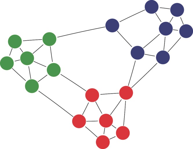
The main advantage of Q _R is that it is agnostic with regard to the measure used to optimize modularity (and even to the method by which the nodes were assigned to modules, which can be arbitrary), as it acts a posteriori, i.e. after nodes have been attributed to modules. It can therefore be used to select the community detection method maximizing modularity. This measure works on most type of networks, as it makes no difference if links are directional, or if the networks are bipartite/unipartite. An illustration of this measure is given in Figure 1. This measure is purposefully simple, (i) so that it makes no assumption about what modularity is, or how it should be optimized, and (ii) because it is not meant to be used to optimize modularity, but to either compare the outcome of different methods, or present the value of modularity in a way that is straightforward to interpretate.

Figure 1. A cartoon depiction of a modular network with links between modules.

Nodes of the same modules are identified by different colors. This network has a modularity (Louvain method) of Q = 0.527. Out of the 36 interactions, 31 are established within modules, and 5 between modules. This gives a Q _R value of 0.86, and Q′ _R = 0.72.

A python implementation of this measure, using the networkx package, is proposed at https://gist.github.com/tpoisot/4947006. It reads data in the edge list format, and offers additional functions to generate null networks, as detailed in the following section.

Example application: realized modularity in ecological networks

In this section, I analyze the modular structure of a large dataset of 290 ecological networks (187 food webs and 113 host-parasite networks) published in previous meta-analyses ^{18, 19}. Modularity is an important feature of ecological interaction networks, which is linked to their resilience ^{20, 21}, stability ⁷, biogeographic structure ²², functioning ²³, and to the evolutionary mechanisms involved in their assembly ²⁴. Notably, the occurrence of interactions between and within modules plays a central role in the structure of pollination networks ⁴, and help buffer the effect of species extinctions ²¹.

The existence of interactions in ecological systems involves a large family of processes, ranging from abudance related ^{25, 26} (abundant species are more likely to interact together) to trait related ²⁷ (pollination depends on the flower and insect having compatible morphologies, predators are constrained by the body-size of their preys). The interaction within these different families of mechanisms will drive heterogeneity in interaction strength ²⁸. Yet, the analysis of binary matrices (is there an interaction between a pair of species, or not), still has relevance to identify properties that are conserved across systems ²⁹, especially given that one could argue that quantitative information on interaction strength is an additional level of information. The systems analyzed in this section are represented by their adjacency matrix, describing the presence or absence of an interaction.

Data and analysis

I used the Louvain method ³⁰ to detect modules, due to its rapidity and efficiency on large networks. The Louvain method works in two steps: first it optimizes modularity locally, through clustering of neighboring nodes. These clusters are, in the second steps, aggregated together, until modularity ceases to increase. This method is known to give values of modularity comparable to what is found using e.g. simulated annealing, and has been observed to give modules that have a functional relevance ³⁰. Once the partition is returned by the Louvain method, I recorded its realized modularity Q′ _R, and its modularity Q (using the Newman and Girvan ³¹ measure).

For each network, I compared the values of Q and Q′ _R on the empirical networks to their random estimate using a network null model. Because random networks will by chance display a modular (among other) structure, it is important to confront the empirical measures of Q and Q′ _R to their random expectations. The null model is defined as follows. For each node n of the network, I measured its degree d _n, its number of successors (the number of node it links to, or generality in ecological terms, as per ³²) g _n, and its number of predecessors (the number of nodes that link to it, or vulnerability) v _n. In each random network, for each pair of nodes ( i, j), the probability that i interacts with j is given by

$$P(i\to j)=\frac{1}{2}\left(\frac{g_i}{d_i}+\frac{v_j}{d_j}\right),\hspace{0.17em}\hspace{0.17em}\hspace{0.17em}\hspace{0.17em}\hspace{0.17em}\hspace{0.17em}\hspace{0.17em}\hspace{0.17em}\hspace{0.17em}\hspace{0.17em}\hspace{0.17em}\hspace{0.17em}\hspace{0.17em}\hspace{0.17em}(3)$$

and conversely for P( j → i). This null model allowed the generation of pseudo-random networks through a Bernoulli process (in each replicate, the occurrence of a link is randomly determined), with the same connectance, and the same distribution of degrees, generality, and vulnerability, as the original one (these properties are also conserved at the node level). For each of the 290 networks, 1000 pseudo-random replicates are generated. For each of them, the average value of Q _R and Q′ _R are estimated along with their 90% confidence interval. When the empirical value lies outside the confidence interval, it can be assumed that the modular structure of the network is different than expected by chance.

Results

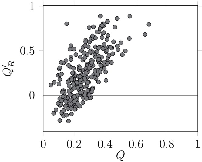
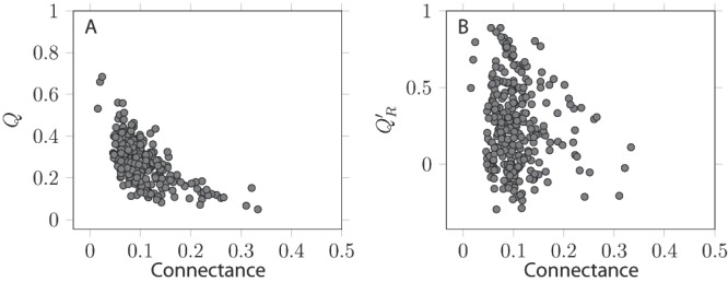
There is a strong, positive relationship, between the values of Q′ _R and the values of Q (Pearsons's product-moment correlation coefficient, as implemented in R 2.15 ³³, ρ = 0.64, 288 d.f., p < 10 ^–6), i.e. networks for which a high modularity is detected tend to have relatively few between-module links ( Figure 2). It is worth noting that some Q′ _R values were negative: in some cases, the best community division resulted in more interactions between than within modules. This result highlights why using an a posteriori measure is useful: other measures of modularity do not reveal the fact that there were more interactions between than within modules. In the dataset examined, most of the networks with a modularity lower than 0.2 had a negative realized modularities. This result suggests that discussing the modularity of such networks makes little sense, as their modules are not more densely linked than other random collections of nodes within the graph. Q and Q′ _R have different relationships with connectance ( Figure 3). Increased connectance values resulted in lower modularity ( ρ = –0.61, 288 d.f., p < 10 ^–6), but had no impact on Q′ _R. This is a desirable property, as it allows easy comparison with the Q′ _R values of networks with extremely different connectances.

Figure 2. Relationship between the modularity of the best partition using the Louvain method and the a posteriori realized modularity.

There exists a strong, positive relationship between the two variables. Worth noting is the fact that, for some networks, the best partition resulted in negative versions of Q′ _R, i.e. there were more interactions between than within modules. Each dot corresponds to a network.

Figure 3. Relationship between the two measures of modularity and network connectance.

A. Q is negatively affected by connectance, i.e. densely connected networks are more likely not to be modular. B. Q′ _R is not affected by connectance, allowing to use it to compare different networks. Each dot corresponds to a network.

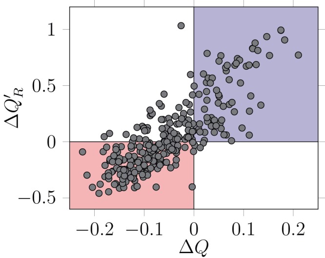
There is a linear relationship between the deviation from random expectation of Q and Q′ _R ( ρ = 0.78, 288 d.f., p < 10 ^–6 – Figure 4). The deviations (respectively Δ Q and Δ Q′ _R) are calculated as the empirical value, minus the average of the values on the networks generated by the null model. As an example, a Δ Q less than zero indicates that the empirical network is less modular than expected by chance. Confidence intervals for the average of the null models were typically very narrow (not represented in the figure to avoid cluttering – see associated original dataset), probably owing to the fact that the null model is restrictive on the type of networks which are generated. It is worth noting that for some networks, the diagnostic of the null model analysis is conflicted. In a vast majority of the situations, this corresponds to networks having a lower modularity than expected by chance, yet having a higher realized modularity (dots in the upper left corner of Figure 4). Depending on whether the true modularity, or the realized modularity, is the most relevant metric of the processes studied, the interpretation of the null models for these networks will be different.

Figure 4. Linear relationship between the deviation from random expectation in Q and Q′ _R.

Networks in the red area are detected as being less modular than expected both by Q′ _R and Q, while networks in the blue area are detected as being more modular. Although the agreement between the two measures is good (see main text for statistics), some networks are detected as having a higher than expected realized modularity Q′ _R, despite a lower than expected modularity Q. Each dot correspond to a network.

Relationships between raw and realized modularity

Relationships between raw and realized modularity for 290 networks, including the results of null models

results.dat

w - web number

q - raw (Louvain) modularity

nm - number of modules

qr - realized modularity

ed - number of edges

no - number of nodes

co - connectance

qe - random expectation of Louvain modularity

eqe - variance of the random modularity expectation

qre - random expectation of realised modularity

eqre - variance of the random realized modularity expectation

rq - rank (based on modularity)

rqr - ranked (based on realized modularity)

dq - empirical - random modularity

dqr - empirical - random realized modularity

 

altmeasures.dat

w - network (unipartite) number

Wa(R) - modularity and realized modularity with the walktrap method

Sp(R) - with the spinglass algorithm

Eb(R) - with the edge-betweenness method

Finally, for the unipartite network dataset, I compare the results of three alternative methods of community detection (the walktrap, spinglass, and edge-betweenness methods, as implemented in the igraph library). For each of the unipartite networks, I computed the value of Barber's Q, and Q′ _R, on the best partition found. The strong correlation between Q and Q′ _R were observed for the spinglass method (r = 0.61, df = 165, t = 10.02), and the weakest for the edge-betweenness method (r = 0.04, non-significant at α = 0.05). The walktrap algorithm gave results in between (r = 0.489, df = 165, t = 7.20). For both the walktrap and edge-betweenness methods, several networks had negative values of Q′ _R, which indicates that the “best” community partition had more links between than within modules. The spinglass method had, by contrast, less than 8% of all networks with values of Q′ _R lower than 0, meaning that this algorithm should be prefered when one wants to group nodes in densely connected clusters.

Conclusions

The Q′ _R measure presented here allows the estimation of the proportion of interactions established between different modules in a network. This measure can be analyzed much in the same way as other measures of modularity, but is applied a posteriori. As such, it can help choose the “best” community partition according to the property of the network that one wants to maximize. For example, choosing the partition giving the lowest Q′ _R can help identify which species are more likely to act as connectors between different modules. Ultimately, this information may have some practical relevance as a decision tool. Saavedra et al. ⁵ showed that different nodes contribute differently to overall network properties. In a context in which networks are increasingly being used as management tools to adress e.g. conservation or pest management ⁸, knowing the realized modularity, and developing methods to estimate which species have the highest impact on it, can allow the design of efficient policies to maximize, or decrease, the ability of network modules to interact.

Funding Statement

TP is funded by a PBEEE-FQRNT post-doctoral scholarship, and thanks the EEC Canada Research Chair for providing computational support.

The funders had no role in study design, data collection and analysis, decision to publish, or preparation of the manuscript.

References

- 1.Espinosa-Soto C, Wagner A: Specialization can drive the evolution of modularity. PLoS Comput Biol. 2010;6(3):e1000719 10.1371/journal.pcbi.1000719 [DOI] [PMC free article] [PubMed] [Google Scholar]
- 2.Bauer-Mehren A, Bundschus M, Rautschka M, et al. : Gene-disease network analysis reveals functional modules in mendelian, complex and environmental diseases. PLoS One. 2011;6(6):e20284 10.1371/journal.pone.0020284 [DOI] [PMC free article] [PubMed] [Google Scholar]
- 3.Fortuna MA, Bonachela JA, Levin SA: Evolution of a modular software network. Proc Natl Acad Sci U S A. 2011;108(50):19985–19989 10.1073/pnas.1115960108 [DOI] [PMC free article] [PubMed] [Google Scholar]
- 4.Olesen JM, Bascompte J, Dupont YL, et al. : The modularity of pollination networks. Proc Natl Acad Sci U S A. 2007;104(50):19891–19896 10.1073/pnas.0706375104 [DOI] [PMC free article] [PubMed] [Google Scholar]
- 5.Saavedra S, Stouffer DB, Uzzi B, et al. : Strong contributors to network persistence are the most vulnerable to extinction. Nature. 2011;478(7368):233–235 10.1038/nature10433 [DOI] [PubMed] [Google Scholar]
- 6.Carstensen DW, Dalsgaard B, Svenning JC, et al. : Biogeographical modules and island roles: a comparison of Wallacea and the West Indies. J Biogeogr. 2012;39(4):739–749 10.1111/j.1365-2699.2011.02628.x [DOI] [Google Scholar]
- 7.Thébault E: Identifying compartments in presence-absence matrices and bipartite networks: insights into modularity measures. J Biogeogr. 2013;40(4):759–768 Ed. by Joseph Veech, n/a-n/a. 10.1111/jbi.12015 [DOI] [Google Scholar]
- 8.Chadès I, Martin TG, Nicol S, et al. : General rules for managing and surveying networks of pests, diseases, and endangered species. Proc Natl Acad Sci U S A. 2011;108(20):8323–8328 10.1073/pnas.1016846108 [DOI] [PMC free article] [PubMed] [Google Scholar]
- 9.Newman ME: Modularity and community structure in networks. Proc Natl Acad Sci U S A. 2006;103(23):8577–82 10.1073/pnas.0601602103 [DOI] [PMC free article] [PubMed] [Google Scholar]
- 10.Zhang XS, Wang RS: Optimization analysis of modularity measures for network community detection. The Second International Symposium on Optimization and Systems Biology.Lijiang, China,2008;13–20 Reference Source [Google Scholar]
- 11.Barber MJ: Modularity and community detection in bipartite networks. Phys Rev E Stat Nonlin Soft Matter Phys. 2007;76(6 Pt 2):066102 10.1103/PhysRevE.76.066102 [DOI] [PubMed] [Google Scholar]
- 12.Liu X, Murata T: Community detection in large-scale bipartite networks. Trans Jpn Soc Artif Intell. 2010;5(1):184–192 10.1527/tjsai.25.16 [DOI] [Google Scholar]
- 13.Marquitti D, Maria F, Roberto GP, Jr, et al. : MODULAR: Software for the Autonomous Computation of Modularity in Large Network Sets.2013;1304(2917): arXiv e-print. Reference Source [Google Scholar]
- 14.Wiederhold G: Mediators in the architecture of future information systems. IEEE Comput Mag. 1992;25(3):38–49 10.1109/2.121508 [DOI] [Google Scholar]
- 15.Leskovec J, Lang KJ, Dasgupta A, et al. : Statistical properties of community structure in large social and information networks. Proceeding of the 17th international conference on World Wide Web - WWW ’08 New York, New York, USA: ACM Press,2008;695 10.1145/1367497.1367591 [DOI] [Google Scholar]
- 16.Hartwel LH, Hopfield JJ, Leibler S, et al. : From molecular to modular cell biology. Nature. 1999;402(6761 Suppl):C47–52 10.1038/35011540 [DOI] [PubMed] [Google Scholar]
- 17.Rosvall M, Bergstrom CT: Maps of random walks on complex networks reveal community structure. Proc Natl Acad Sci U S A. 2008;105(4):1118–23 10.1073/pnas.0706851105 [DOI] [PMC free article] [PubMed] [Google Scholar]
- 18.Gravel D, Massol F, Canard E, et al. : Trophic theory of island biogeography. Ecol Lett. 2011;14(10):1010–1016 10.1111/j.1461-0248.2011.01667.x [DOI] [PubMed] [Google Scholar]
- 19.Poisot T, Canard E, Mouillot D, et al. : The dissimilarity of species interaction networks. Ecol Lett. 2012;15(12):1353–1361 10.1111/ele.12002 [DOI] [PubMed] [Google Scholar]
- 20.Fortuna MA, Stouffer DB, Olesen JM, et al. : Nestedness versus modularity in ecological networks: two sides of the same coin? J Anim Ecol. 2010;79(4):811–817 10.1111/j.1365-2656.2010.01688.x [DOI] [PubMed] [Google Scholar]
- 21.Stouffer DB, Bascompte J: Compartmentalization increases food web persistence. Proc Natl Acad Sci U S A. 2011;108(9):3648–3652 10.1073/pnas.1014353108 [DOI] [PMC free article] [PubMed] [Google Scholar]
- 22.Flores CO, Valverde S, Weitz JS: Multi-scale structure and geographic drivers of cross-infection within marine bacteria and phages. ISME J. 2013;7(3):520–532 10.1038/ismej.2012.135 [DOI] [PMC free article] [PubMed] [Google Scholar]
- 23.Thébault E, Loreau M: Food-web constraints on biodiversity-ecosystem functioning relationships. Proc Natl Acad Sci U S A. 2003;100(25):14949–14954 10.1073/pnas.2434847100 [DOI] [PMC free article] [PubMed] [Google Scholar]
- 24.Flores CO, Meyerb JR, Valverdec S, et al. : Statistical structure of host-phage interactions. Proc Natl Acad Sci U S A. 2011;108(28):E288–297 10.1073/pnas.1101595108 [DOI] [PMC free article] [PubMed] [Google Scholar]
- 25.Bluthgen N, Menzel F, Bluthgen N: Measuring specialization in species interaction networks. BMC Ecol. 2006;6:9 10.1186/1472-6785-6-9 [DOI] [PMC free article] [PubMed] [Google Scholar]
- 26.Canard E, Mouquet N, Marescot L, et al. : Emergence of structural patterns in neutral trophic networks. PLoS One. 2012;7(8):e38295 10.1371/journal.pone.0038295 [DOI] [PMC free article] [PubMed] [Google Scholar]
- 27.Bartomeus I: Understanding linkage rules in plant-pollinator networks by using hierarchical models that incorporate pollinator detectability and plant traits. PLoS One. 2013;8(7):e69200 10.1371/journal.pone.0069200 [DOI] [PMC free article] [PubMed] [Google Scholar]
- 28.Berlow EL, Navarrete SA, Briggs CJ, et al. : Quantifying variation in the strengths of species interactions. Ecology. 1999;80(7):2206–2224 10.1890/0012-9658(1999)080[2206:QVITSO]2.0.CO;2 [DOI] [Google Scholar]
- 29.Dunne JA: The Network Structure of Food Webs. In: Ecological networks: Linking structure and dynamics.Ed. by Jennifer A Dunne and Mercedes Pascual. Oxford University Press,2006;27–86 Reference Source [Google Scholar]
- 30.Blondel VD, Guillaume JL, Lambiotte R, et al. : Fast unfolding of communities in large networks. J Stat Mech Theory Exp. 2008;2008(10):P10008 10.1088/1742-5468/2008/10/P10008 [DOI] [Google Scholar]
- 31.Newman ME, Girvan M: Finding and evaluating community structure in networks. Phys Rev E Stat Nonlin Soft Matter Phys. 2004;69(2 Pt 2):026113 10.1103/PhysRevE.69.026113 [DOI] [PubMed] [Google Scholar]
- 32.Schoener TW: Food webs from the small to the large. Ecology. 1989;70(6):1559–1589 10.2307/1938088 [DOI] [Google Scholar]
- 33.R. Development Core Team. R: A Language and Environment for Statistical Computing. Vienna, Austria,2010. Reference Source [Google Scholar]