Computer-Aided Segmentation System for Breast MRI Tumour using Modified Automatic Seeded Region Growing (BMRI-MASRG)

Abstract

In this paper, an automatic computer-aided detection system for breast magnetic resonance imaging (MRI) tumour segmentation will be presented. The study is focused on tumour segmentation using the modified automatic seeded region growing algorithm with a variation of the automated initial seed and threshold selection methodologies. Prior to that, some pre-processing methodologies are involved. Breast skin is detected and deleted using the integration of two algorithms, namely the level set active contour and morphological thinning. The system is applied and tested on 40 test images from the RIDER breast MRI dataset, the results are evaluated and presented in comparison to the ground truths of the dataset. The analysis of variance (ANOVA) test shows that there is a statistically significance in the performance compared to the previous segmentation approaches that have been tested on the same dataset where ANOVA p values for the evaluation measures’ results are less than 0.05, such as: relative overlap (p = 0.0002), misclassification rate (p = 0.045), true negative fraction (p = 0.0001) and sum of true volume fraction (p = 0.0001).

Introduction

Magnetic resonance imaging (MRI) has been widely used for medical breast screening since MRI provides better contrast for the breast soft tissues when compared to mammogram and ultrasound images. Although this is valuable information, the presented data still needs to be interpreted by the radiologist [1]. Computer-aided detection (CAD) systems are used with image processing algorithms to assist MRI radiologists in improving the quality of the breast MRIs, detecting the tumour masses and to reduce the number of false-positive diagnoses [2].

CAD algorithms are developed to detect breast tumours [3, 4]. Several techniques for medical image segmentation exist. These include methods such as particle swarm optimization [5], genetic algorithms [6] and artificial fuzzy logic [7–9].

The supervised, unsupervised and semi-supervised methods are explored in Azmi et al.’s study [10]. In their comparison study on the MRI breast reference image database to evaluate response (RIDER) dataset, they found that the supervised segmentation methods such as k-nearest neighbour (KNN), support vector machine (SVM) and Bayesian while the semi-supervised method such as self training and improved self training (IMPST) lead to high accuracy. However, labelled data is needed. Hence, the process becomes difficult, expensive, and involves a lot of time. On the other hand, unsupervised methods such as; fuzzy C-means (FCM) need no prior knowledge but their performance is low [10].

The seeded region growing (SRG) algorithm which was proposed by Adams and Bischof [11] is widely used in medical images today because it effectively segments different types of images. According to empirical studies of the efficiency of the seeded region growing on MRI brain segmentation, the results are promising for both light and dark abnormalities. Nevertheless, a lower performance in dark abnormalities segmentation is produced as it has slightly lower correlation values in all conditions as compared to light abnormalities [12, 13].

In Meinel’s study on MRI breast segmentation [14], the SRG was also used. The experiments on breast tumour segmentation returned robust results. However, this approach needed an initial threshold value to be specified by the user, which is then used to find the anticipated locations of the tumours.

The SRG feature extraction (SRGFE) algorithm has been proposed on cervical cancer screening. This algorithm extracted four cervical cells features: size of nucleus, cytoplasm, grey level of nucleus, and cytoplasm. The data extracted using SRGFE algorithm gave high correlation values when compared with data extracted manually. Still, the user needs to determine the region of interest to select the initial seed pixel. The user also needs to determine the threshold value [15].

Wu et al. proposed texture feature-based automated SRG algorithm on abdominal organ segmentation [16]. The advantage of this algorithm is that it allows minimum user intervention. This is helpful for batch work. However, this approach does have drawbacks. Texture feature-based methods all have the assumption that the region should have texture homogeneity. For organs with complex texture, this approach may not work well.

Shan et al. proposed an automatic seed point selection algorithm for seeded region growing on ultrasound breast images [17]. The algorithm needs no prior information or training processes. Both the homogeneous texture features and spatial features of the breast tumours are taken into account. However, some cases failed because of the shadowing effects of areas which have similar intensity as the tumour and also right below the tumour.

In this study, a proposed CAD with automated features for MRI breast tumour segmentation is presented using a modified SRG technique. The proposed approach tries to avoid user interaction; the system automatically generates the regions of interest, SRG initial seed and SRG threshold values using new algorithms.

Methods

The methodology starts with a pre-processing stage, followed by the detection of the breast skin and deletion phase. Then, it ends with tumour segmentation stage using SRG with proposed methods for automatic seed and threshold values selection procedures. The whole perspective is shown in Fig. 1.

Fig. 1.

Methodology flowchart

Image Pre-Processing

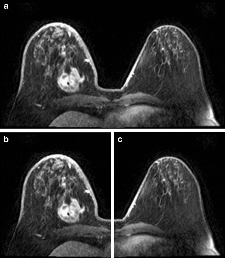
The pre-processing phase is the first process that is executed. The image is split into two sub-images; the right breast image and the left breast image. This process is used only if the MRI breast image is axial (i.e. the image is taken from the perspective of the patient from head to toe). This process is skipped if the image is sagittal (i.e. the image is taken according to the lateral view) because of the fact that the sagittal image shows only one side of the breast, i.e. either the right or the left. Therefore, the splitting process in the case of the sagittal image is not necessary. The splitting process can be done by finding the middle of the x-coordinate of the image and splitting the image vertically from that point. Figure 2 shows the image splitting process. The median filter is then applied. The usage of the median filter here is to reduce the salt and pepper noise while the boundaries and features are kept intact [18].

Fig. 2.

Results of image splitting; a Original image. b Left side. c Right side

Breast Skin Detection and Deletion

The purpose of this process is to delete the breast skin area which has similar intensity range compared to the tumour area’s intensity range. This process is also necessary in order to facilitate a better automatic seed selection for the tumour segmentation in the next stage. To delete the breast skin, an integration of level set active contour algorithm [19] with morphological thinning algorithm is used in this phase. The level set active contour algorithm is used to detect the breast skin border; the morphological thinning algorithm is used to delete the detected breast skin border.

Level set formulation without re-initialization (which is specially known as Chunming’s algorithm) is included as one of the active contour’s detection algorithms. Active contours are dynamic curves that move toward the mass border. An external energy moves the zero level curves toward the mass border using the edge indicator function g that is defined in Eq. (1).

1

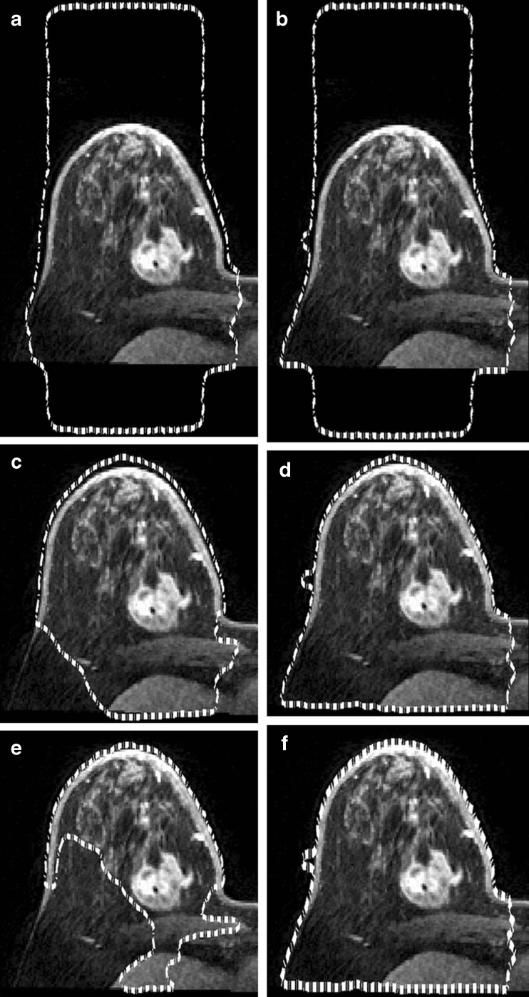
where I is the image and Gσ is the Gaussian kernel with a standard deviation σ. By changing the σ parameter value and the number of the iterations N_LS, the resultant detection is changed. Figure 3 shows the different results after Chunming’s algorithm is applied with different values of σ and N_LS.

Fig. 3.

Different results after applied Chunming’s algorithm with different values of σ and N _LS. a σ = 3, N _LS = 100; b σ = 1.5, N _LS = 100; c σ = 3, N _LS = 300; d σ = 1.5, N _LS = 300; e σ = 3, N _LS = 700; f σ = 1.5, N = 700

The parameters have been selected using the trial and error method, whereby a higher number of iterations N_LS give better detection. Therefore, the best value for N_LS is 700 while the best value of σ is 1.5 [20]. These choices of the values are generic for all breast MRI images after resizing the images to be 288 × 288 pixels. In order to delete the detected breast skin border, the morphological thinning algorithm is used. The algorithm is divided into two sub-iterations as described in [21]. The image is divided into two distinct sub-fields. Then in the first sub-iteration, pixel p from the first sub-field is deleted if and only if the first three conditions as shown below are true. In the second sub-iteration, pixel p from the second sub-field is deleted if and only if, the first two and fourth conditions are true.

First condition:

2

where

3

4

x₁, x₂, …, x₈ are the values of the eight neighbours of p, starting with the east neighbour and numbered in counter-clockwise order.

Second condition:

5

where

6

7

Third condition:

8

Forth condition:

9

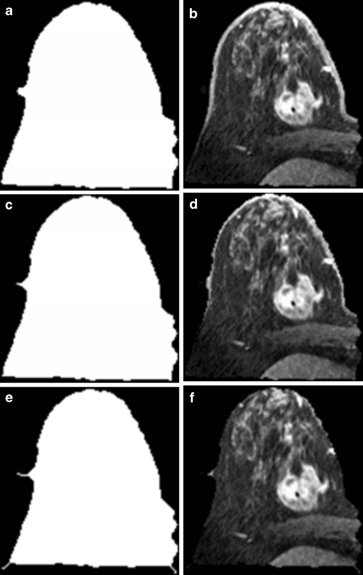
The two sub-iterations formulate the main iteration of the thinning algorithm. The thinning level depends on the number of iterations. Whenever the number of iterations is increased, there would be more shrinking of the image’s border. The morphological thinning algorithm only accepts a binary version of the image. Therefore, the resultant image after the Chunming’s algorithm would be converted to a binary image. Furthermore, after applying the thinning, the binary image is reconverted into its original grey scale representation. Figure 4 shows the results after the morphological thinning algorithm is applied using three different iteration numbers (N_Th = 1, N_Th = 3 and N_Th = 7). From Fig. 4, N_Th = 7 is the best iteration number which enables the thinning algorithm whereby the deleted amount of pixels equals the thickness of the breast skin.

Fig. 4.

Results after applying morphological thinning algorithm with three different iteration numbers on the resultant image of Chunming’s algorithm; a after applying thinning (N _Th = 1) on binary image; b after reconverting thinning image (N _Th = 1) to its original grey scale; c after applying thinning (N _Th = 3) on binary image; d after reconverting thinning image (N _Th = v3) to its original grey scale; e after applying thinning (N _Th = 7) on binary image; f after converting thinning image (N _Th = 7) to its original grey scale

Tumour Segmentation

In this study, the SRG algorithm [11] for tumour segmentation is chosen because it is fast, simple and robust. SRG has two variable factors which are usually manually selected. The first factor is determining the initial seed pixel that the SRG can begin to grow. The second factor is the threshold value for measuring the difference between the pixel and its neighbours. In this work, an automated version of the seed selection algorithm consisting of five steps and an automated SRG threshold value comprising of four steps are proposed.

Automatic Seed Selection

The steps taken for this process are as follows:

1. Minimise the selection search regions by finding the suspected regions first by thresholding. The mean maximum raw thresholding algorithm (MMRT) is proposed in this work based on an automatic selection for the suitable threshold value that separates the image into white and black regions. The algorithm searches for the maximum value in each row in the image and saves it temporarily. This process is repeated for all the rows until the last. Then a summation of the temporarily stored values is calculated. The mean maximum raw is then calculated by dividing the summation value by the number of rows in the image. As described in Eq. (10).

   10

   Where i is the first row in the image, N is the number of row, and M is the maximum intensity pixel value in the row.

   The resultant mean value will be considered as the threshold value for the binarization process. This divides the image into two intensity regions, i.e. the black region is below the (mean max raw) value while the white region would be above the same value. Applying morphological open operation (erosion followed by dilation operations) would remove the unwanted small white speckles in the image which do not belong to the tumour regions and to enhance the boundary of the suspected regions.

2. Measure two of the region properties for each suspected region which results from step 1. The properties are the mean intensity value of pixels and the area which refers to the number of the pixels of the region. These selected properties are related to the tumour features. Before the property measuring process, it is necessary to revert the original grey level representation to the suspected regions (which has become white after the thresholding process). This process can be done by multiplying the binarised image matrix with the original image matrix.

3. Calculate the densities of the regions’ intensity by dividing the area of each region with the mean intensity of the same region.

   

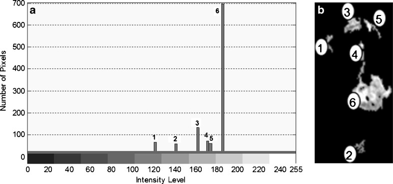
4. Rank the suspected regions by their density values that have been calculated in step 3. The highest region’s density value will be chosen as the main suspected region (SR) to search for the seed pixel within it. Figure 5a shows an example for the ranked regions based on their density value. Figure 5b shows the bar chart for the ranked regions that indicate region number 6 (whereby the intensity value is around 186) as the highest region’s density value.

5. Search for the maximum intensity value pixel from the main suspected region. This is because the tumour region is the region having the highest intensity area amongst other regions in the breast images.

Fig. 5.

Region ranking according to their pixels’ density values. a Image regions flags. b Bar chart for the ranked regions according to the highest mean intensity values

Automatic SRG Threshold Value Selection

The Automatic SRG threshold value selection approach is based upon an estimated value. This is in accordance to the difference between the mean intensity of the main suspected region and the mean intensity for the other whole breast regions that are neighbouring the main suspected region, except for the breast skin. The approach comprises of four steps which are shown as below:

1. Find the mean intensity value (MeanInts_SR) for the main SR (that has been detected in the previous section, step 4).

2. Isolate the neighbouring area of the SR from the other unwanted regions such as; the black background, the breast skin (which was detected earlier in the methodology) and SR itself. This is as stated in Eq. 12.

   12

3. Find the mean intensity for the Neighboring_Area which is called here as (MeanInts_NA).

4. Calculate the SRG threshold (SGR_Thr) using the following Eq. 13.

   13

Seeded Region Growing

This method starts with an initial seed pixel and tries to compare its neighbourhood pixels with the seed according to some attributes, such as the intensity or texture. It then merges them if they are similar enough.

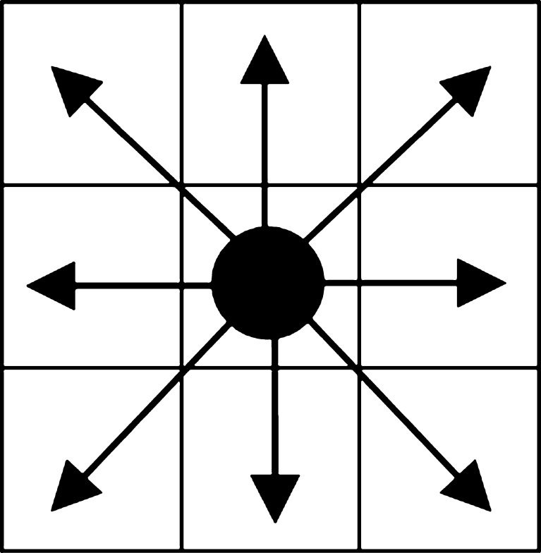
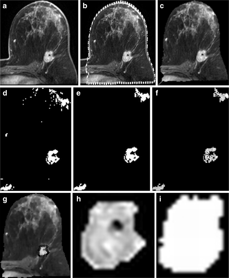
In this study, after the proper initial pixel seed is selected, the eight neighbouring pixels will be tested according to SRG threshold value (which has been detected in the previous section). The neighbouring pixel is considered to be in the segmented region if it is above the threshold value. Subsequently, the eight neighbours of the new pixel will be tested and sorted too. The process then continues in the same manner. Figure 6 shows the initial seed pixel and the eight neighbours. The different processing steps of the proposed methodology are shown in Fig. 7.

Fig. 6.

The initial seed pixel and its eight neighbouring pixels

Fig. 7.

The proposed system approach processes on one of the RIDER images: a original image; b breast skin detection after applying level set algorithm; c breast skin deletion after applying the thinning algorithm; d after applying the thresholding process using MMRT algorithm; e after applying morphological open operation; f initial seed selected using the proposed method (star sign (*)); g after the SRG method is applied using the proposed method of SRG threshold value; h The segmented tumour regions; i GT of the image

Evaluation Criteria

Different measures are used in this study in order to evaluate the segmentation accuracy. The number of pixels of (R_S) and (R_T) have to be found first, where (R_S) represents the segmented region by the proposed approach, while (R_T) represents the ground truth regions segmented by the experts.

The first evaluation methodology used in this study is the true positive fraction (TPF) (also called sensitivity), false negative fraction (FNF) (also called specificity), false positive fraction (FPF), true negative fraction (TNF) and sum of true volume fraction (STVF). The calculations are made using Eqs. 14–18 [22–25].

14

15

16

17

18

Another methodology is also used here, i.e. the relative overlap (RO) and misclassification rate (MCR) which have been used before for brain segmentation [26] and in breast segmentation [10, 27]. The RO (also called segmentation precision) is calculated in Eq. 19

19

The MCR is calculated in Eq. 20

20

The final tumour segmentation results are compared with the ground truth (GT) of the dataset (shown in Fig. 7f–j).

To evaluate the automatic seed selection, the positions of the seed pixel that have been selected by the proposed approach are compared with the reference’s position. The reference’s position is manually selected according to the GT.

21

Where p_m is the (x, y) coordinates of the manual selected seed pixel and p_a is the (x, y) coordinates of the automatic selected seed pixel.

Results

The methodology explained earlier is applied and tested on the RIDER breast MRI dataset which is downloaded from the National Biomedical Imaging Archive [28]. This website belongs to the US National Cancer Institute. The dataset also include GT segmentation, which have been identified manually by expert radiologists. Forty images (24 malignant and 16 benign) from the dataset with their GTs are used in the experiments as test images. GT is used as a benchmark for performance evaluation of segmentation methods in our experiments. All images are axial 288 × 288 pixels.

The two evaluation methodologies explained in the evaluation criteria section are then applied. The results are tabulated in Tables 1 and 2. Table 1 illustrates the results of the first evaluation methodology (Eqs. (14)–(18)).

Table 1.

Results of true positive fraction (TPF), false negative fraction (FNF), false positive fraction (FPF), true negative fraction (TNF), and sum of true volume fraction (STVF)

Patient No.	TPF (sensitivity)	FNF (specificity)	FPF	TNF	STVF
Mean	0.8233	0.1767	0.0976	0.9023	1.7256
Stddev	0.0965	0.0965	0.0970	0.0969	0.1040
Max	0.9944	0.4779	0.3523	0.9938	1.8669
Min	0.5221	0.0045	0.0001	0.6477	1.4632

Table 2.

Results of relative overlap (RO) and misclassification rate (MCR)

	RO	MCR
Mean	0.7524	0.1767
Stddev	0.0848	0.0965
Max	0.8754	0.4779
Min	0.4931	0.0045

Table 2 shows the results of the second evaluation methodology (Eqs. (19) and (20)), where the mean of RO for all of the images is high, which is about 0.7524 and the mean of MCR is low, which is about 0.1767.

Table 3 shows the automatically selected initial seed pixel’s coordinates when compared with the manually selected pixel’s coordinates. The manually selections are made according to the position of the segmented tumours in the GT. The calculations have been made using equation (19). Results obtained in Table 3 indicate that accuracy of the x and y coordinates are very precise; as x and y accuracy means are 97.38 and 97.08, respectively.

Table 3.

Automatically selected initial seed pixel’s coordinates compared with the manually selected pixel’s coordinates

	x Accuracy (%)	y Accuracy (%)
Mean	97.38	97.08
Sddtev	1.550	2.890
Max	98.92	99.43
Min	90.80	80.83

The results of the proposed approach are compared with the results of previous works involving five different segmentation approaches. The previous work’s results have been stated in the comparison study of Azmi et al. [10]. The approaches are KNN, SVM, Bayesian, FCM and IMPST. The tested data are the same dataset (Breast MRI RIDER dataset). The measures used for the evaluation are RO, MCR, TPF (sensitivity), TNF and STVF. The results of the five approaches and the proposed approach are stated in Table 4.

Table 4.

Segmentation results for the proposed approach and other approaches (KNN, SVM, Bayesian, FCM and IMPST)

Method	Statistic	TPF	TNF	STVF	RO	MCR
KNN	Mean	0.73	0.75	1.49	0.60	0.27
	Stddev	0.13	0.15	0.19	0.12	0.10
	Max	0.87	0.97	1.75	0.76	0.58
	Min	0.42	0.99	1.85	0.36	0.13
SVM	Mean	0.75	0.71	1.46	0.60	0.25
	Stddev	0.19	0.21	0.31	0.19	0.12
	Max	0.94	0.99	1.85	0.86	0.70
	Min	0.30	0.17	0.67	0.26	0.06
Bayesian	Mean	0.76	0.59	1.34	0.56	0.24
	Stddev	0.19	0.25	0.35	0.17	0.08
	Max	0.95	0.97	1.76	0.77	0.70
	Min	0.30	0.09	0.69	0.22	0.05
FCM	Mean	0.82	0.42	1.24	0.59	0.18
	Stddev	0.27	0.55	0.71	0.25	0.08
	Max	0.99	0.96	1.83	0.84	1.00
	Min	0	−0.73	−0.19	0	0.01
IMPST	Mean	0.79	0.83	1.61	0.68	0.21
	Stddev	0.19	0.15	0.21	0.17	0.12
	Max	0.96	0.99	1.88	0.89	0.62
	Min	0.38	0.58	1.18	0.34	0.04
Proposed approach	Mean	0.82	0.90	1.73	0.75	0.18
	Stddev	0.10	0.10	0.10	0.09	0.10
	Max	0.99	0.99	1.87	0.88	0.48
	Min	0.52	0.65	1.46	0.49	0.01

Statistical Analysis

The analysis of variance test (ANOVA) has been applied to make statistical comparison between the proposed approach’s results and the previous methods’ results by finding the level of statistical significance (p). The difference between the groups are considered of significance if (p < 0.05).

From Table 5, it can be seen that there are statistically significant differences between methods (p < 0.05) as determined by one-way ANOVA for OR (F = 5.5429, p = 0.0002); MCR (F = 2.365, p = 0.045); TNF (F = 9.2330, p = 0.0001) and STVF (F = 8.598, p = 0.0001), while there is no significant difference for TNF (F = 0.9479, p = 0.4540).

Table 5.

Summary of the ANOVA tests analysis for the proposed approach’s results comparing with the results of the other approaches (KNN, SVM, Bayesian, FCM and IMPST)

	OR	MCR	TPF	TNF	STVF
F statistic	5.5429	2.365	0.9479	9.2330	8.598
p Value	0.0002	0.045	0.4540	0.0001	0.0001

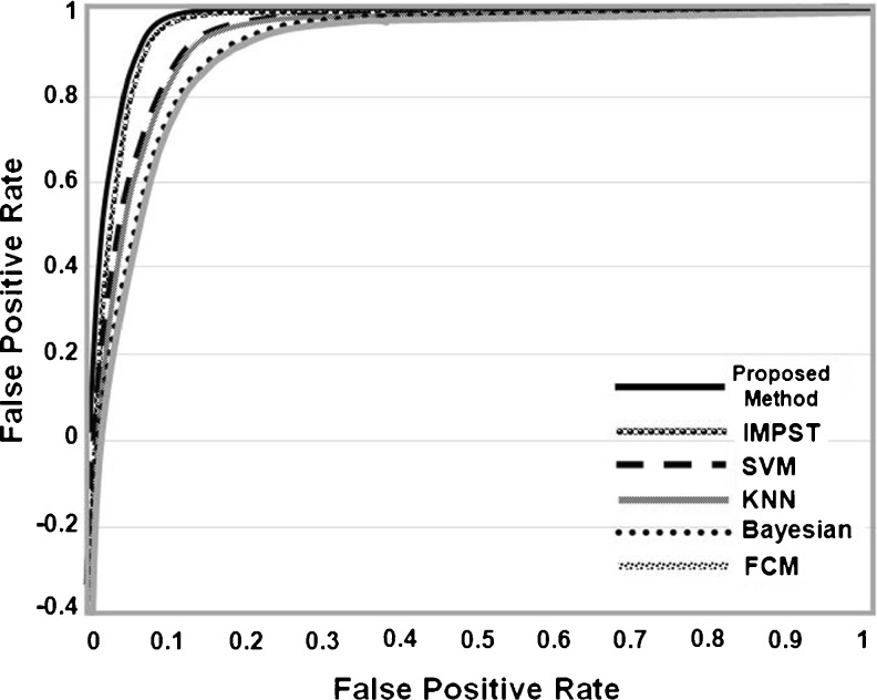
For a more statical evaluation, the receiver operating characteristic (ROC) curve analysis is used to illustrate the TPF rate compared with the FPF rate for the proposed method in comparison with previous methods as shown in Fig. 8. From the area under the curve (AUC) where the high AUC indicates improved segmentation performance, a higher value of TPF is achieved at each value of FPF. The AUC results are listed in Table 6. It can be observed that AUC is 0.97 for the proposed method which is equal to the AUC for IMPST and higher than the other methods.

Fig. 8.

The ROC curves for the proposed method and the previous methods

Table 6.

Area under the curve (AUC) for the proposed approach and other approaches (KNN, SVM, Bayesian, FCM and IMPST)

Method	AUC
KNN	0.95
SVM	0.95
Bayesian	0.94
FCM	0.94
IMPST	0.97
Proposed method	0.97

Discussion and Conclusions

The proposed approach not only provides improved performance, it also facilitates automated selection of the suspected regions without the need to manually select the region of interest (ROI) as is necessary in the previous approaches.

A CAD system with automated features for MRI breast tumour segmentation has been presented in this paper. The methodology of this system is divided into three main stages; i.e. the first stage is the pre-processing, for splitting the axial images and noise reduction. The second stage is the breast skin detection and deletion using the integration of two algorithms, which are level set active contour and morphological thinning. This process is vital because of the similarity of the intensity of the breast skin and the tumour in several cases. The experimental results at this stage show that all of the breast skins are correctly removed from the images.

The final stage is the tumour segmentation based on the modified seeded region growing method. Modification has been made by proposing two automatic approaches for selecting the SRG variable factors which are usually manually selected. The first approach selects the position of the initial seed pixel along while the second approach determines the SRG threshold value by measuring the difference between the initial pixel and its neighbours. The study is then supported by the results of applying the methodology on 40 test images from the RIDER breast MRI dataset.

The results of the evaluation and statistical analysis showed improved performance in general; Table 4 shows improved results when compared with the other approaches. The RO mean of the proposed approach which is 0.75, is higher than the RO mean of IMPST (the best RO mean from the previous approaches) which is 0.68. The TNF mean of the proposed approach is 0.90, which is higher than the TNF mean of IMPST (the best TPF mean of previous approaches) having a value of 0.83. However, the TPF mean of the proposed approach is 0.82, which is almost equal the TPF mean of FCM whose value is 0.82 but is still higher than the TPF mean of the rest of the approaches (KNN, SVM, Bayesian and IMPST). While the statistical analysis of ANOVA shows there are statistically significant differences between the methods where p value is less than 0.05. The p value as tabled in Table 5 for different measures are OR (p = 0.0002), MCR (p = 0.045), TNF (p = 0.0001) and STVF (p = 0.0001), while there is no significant difference for TNF (p = 0.4540).

Not only is the performance significantly improved; the proposed approach also avoided the need for manual selection of the suspected ROI, seed pixel and threshold value processes. Those processes are replaced with automated methods and are generic for any grey scale representation of the breast MRI images. In the previous methods, manual selection of ROI is needed to select the suspected window before the segmentation process can proceed as opposed to the proposed approach.

The problems of the need of human interaction to select the initial seed positions and the threshold value for the SRG algorithm are handled by the proposed approach; by the presented two automatic methods, the first being to select the most suitable initial seed (Table 3 shows the accuracy of the automatic seed position selection) while the subsequent method is used to select the best SRG threshold value. This is also important because the range of the greyscale representations for the tumour and the other parts of the breast is not consistent from one image to another. Therefore, the proposed method has the capability of changing the SRG threshold value according to the respective image’s grey scale distribution.

The Limitations and Future Work

Although this work has achieved its aims, the work is still limited and confined to the automatic segmentation of the breast MRI tumour. The study does not extend beyond, i.e.to classify the types of the tumour (either benign or malignant). Type classification process for the segmented tumour of the proposed approach could be considered as future work to be studied by researchers. Another area would be to apply the same segmentation approach on images of other parts of the body and other modalities of breast screening.

References

- 1.Gardiner I: CAD improves breast MRI workflow: increasing throughput while maintaining accuracy in breast MRI reads requires powerful workflow tools, 2010
- 2.Lehman CD, Peacock S, DeMartini WB, Chen X. A new automated software system to evaluate breast MR examinations: improved specificity without decreased sensitivity. Am J Roentgenol. 2006;187:51–56. doi: 10.2214/AJR.05.0269. [DOI] [PubMed] [Google Scholar]
- 3.Li L, Clark RA, Thomas JA. Computer-aided diagnosis of masses with full-field digital mammography. Acad Radiol. 2002;9:4–12. doi: 10.1016/S1076-6332(03)80290-8. [DOI] [PubMed] [Google Scholar]
- 4.Verma B, Zakos J. A computer-aided diagnosis system for digital mammograms based on fuzzy-neural and feature extraction techniques. IEEE Trans Inf Technol Biomed. 2001;5:46–54. doi: 10.1109/4233.908389. [DOI] [PubMed] [Google Scholar]
- 5.Ibrahim S, Khalid NEA, Manaf M. Empirical study of brain segmentation using particle swarm optimization. Selangor: Shah Alam; 2010. [Google Scholar]
- 6.Ganesan R, Radhakrishnan S. Segmentation of computed tomography brain images using genetic algorithm. Int J Soft Comput. 2009;4:157–161. [Google Scholar]
- 7.Hussain R, Arif S, Sikander MA, Memon AR. Fuzzy clustering based malignant areas detection in noisy breast magnetic resonant (MR) images. Int J Acad Res. 2011;3(2):64. [Google Scholar]
- 8.Kannan S, Sathya A, Ramathilagam S. Effective fuzzy clustering techniques for segmentation of breast MRI. Soft computing—a fusion of foundations. Methodol Appl. 2011;15:483–491. [Google Scholar]
- 9.Noor NM, Khalid NEA, Hassan R, Ibrahim S, Yassin IM: Adaptive Neuro-Fuzzy Inference System for Brain Abnormality Segmentation, 2010
- 10.Azmi R, Anbiaee R, Norozi N, Salehi L, Amirzadi A. IMPST: a new interactive self-training approach to segmentation suspicious lesions in breast MRI. J Med Signals Sens. 2011;1:138–148. [PMC free article] [PubMed] [Google Scholar]
- 11.Adams R, Bischof L. Seeded region growing. IEEE Trans Pattern Anal Machine Intell. 1994;16:641–647. [Google Scholar]
- 12.Khalid NEA, Ibrahim S, Manaf M, Ngah UK: Seed-Based Region Growing Study for Brain Abnormalities Segmentation. Proc. Information Technology (ITSim), 2010 International Symposium: City, 15–17 June 2010 Year
- 13.Ibrahim S, Khalid NEA, Manaf M, Ngah UK. Particle swarm optimization vs seed-based region growing: brain abnormalities segmentation. Int J Artif Intell. 2011;7:174–188. [Google Scholar]
- 14.Meinel LA: Development of computer-aided diagnostic system for breast MRI lesion classification. Dissertation. University of Iowa, Biomedical Engineering, PhD (Doctor of Philosophy), dissertation 2005
- 15.Mat-Isa NA, Mashor MY, Othman NH. Seeded region growing features extraction algorithm; its potential use in improving screening for cervical cancer. Int J Comput Internet Manag. 2005;13(1):61–70. [Google Scholar]
- 16.Wu J, Poehlman S, Noseworthy MD, Kamath MV: Texture feature based automated seeded region growing in abdominal MRI segmentation. Proc. BioMedical Engineering and Informatics BMEI 2008: City, 27–30 May 2008 Year
- 17.Shan J, Cheng HD, Wang Y: A novel automatic seed point selection algorithm for breast ultrasound images. Proc. Pattern Recognition, 2008 ICPR 2008 19th International Conference: City, 8–11 Dec. 2008 Year
- 18.Chun-yu N, Shu-fen L, Ming Q: Research on Removing Noise in Medical Image Based on Median Filter Method, 2009
- 19.Li C, Xu C, Gui C, Fox MD: Level set evolution without re-initialization: a new variational formulation. Proc. Proceedings of the International Conference on Computer Vision and Pattern Recognition: City
- 20.Al-Faris AQ, Ngah UK, Isa NAM, Shuaib IL: MRI breast skin-line segmentation and removal using integration method of level set active contour and morphological thinning algorithms. Journal of Medical Sciences, 2013
- 21.Lam L, Seong-Whan L, Suen CY. Thinning methodologies—a comprehensive survey. IEEE Trans Pattern Anal Mach Intell. 1992;14:879. [Google Scholar]
- 22.Chalana V, Kim Y. A methodology for evaluation of boundary detection algorithms on medical images. IEEE Trans Med Imaging. 1997;16:642–652. doi: 10.1109/42.640755. [DOI] [PubMed] [Google Scholar]
- 23.Fenster A, Chiu B: Evaluation of segmentation algorithms for medical imaging. Proc. Proceedings of IEEE 27th Annual Conference of the Engineering in Medicine and Biology Society: City, September 1–4 Year [DOI] [PubMed]
- 24.Metz CE. ROC methodology in radiologic imaging. Invest Radiol. 1986;21:720–733. doi: 10.1097/00004424-198609000-00009. [DOI] [PubMed] [Google Scholar]
- 25.McNeil BJ, Hanley JA. Statistical approaches to analysis of receiver operating characteristic (ROC) curves. Med Decis Making. 1984;14:137–150. doi: 10.1177/0272989X8400400203. [DOI] [PubMed] [Google Scholar]
- 26.Song T, et al. A hybrid tissue segmentation approach for brain MR images. Med Biol Eng Comput. 2006;44:242. doi: 10.1007/s11517-005-0021-1. [DOI] [PubMed] [Google Scholar]
- 27.Ertas G, Gülçür HO, Osman O, Osman NU, Tunaci M, Dursun M. Breast MR segmentation and lesion detection with cellular neural networks and 3D template matching. Comput Biol Med. 2008;38(10):116–126. doi: 10.1016/j.compbiomed.2007.08.001. [DOI] [PubMed] [Google Scholar]
- 28.US National Cancer Institute: reference image database to evaluate therapy response (RIDER) MRI breast, 2007