A fusion-based approach for uterine cervical cancer histology image classification

Abstract

Expert pathologists commonly perform visual interpretation of histology slides for cervix tissue abnormality diagnosis. We investigated an automated, localized, fusion-based approach for cervix histology image analysis for squamous epithelium classification into Normal, CIN1, CIN2, and CIN3 grades of cervical intraepithelial neoplasia (CIN). The epithelium image analysis approach includes medial axis determination, vertical segment partitioning as medial axis orthogonal cuts, individual vertical segment feature extraction and classification, and image-based classification using a voting scheme fusing the vertical segment CIN grades. Results using 61 images showed at least 15.5% CIN exact grade classification improvement using the localized vertical segment fusion versus global image features.

1. Introduction

Annually, there are 400,000 new cases of invasive cervical cancer out of which 15,000 occur in the U.S. alone [1]. Cervical cancer is the second most common cancer affecting women worldwide and the most common in developing countries. Cervical cancer can be cured in almost all patients, though, if detected early and treated. However, cervical cancer incidence and mortality remain high in resource-poor regions, where high-quality screening programs often cannot be maintained because of inherent complexity. An alternative and more economically feasible screening method uses analysis of visual color change of cervix tissues when exposed to acetic acid. Cervicography is a variation of this technique that augments visual screening by recording a film image of the acetic acid-treated cervix, and has been widely used over the last few decades [2]. The National Cancer Institute (NCI) has collected a vast amount of visual cervicography information, 100,000 cervigrams (digitized 35 mm color slides), obtained by screening thousands of women by this technique. In addition, for several thousand women who were biopsied during this screening, digitized uterine cervix histology images have been collected. This has allowed the development of a unique web-based database of digitized cervix images, which may be used for investigating the role of human papillomavirus (HPV) in the development of cervical cancer and its intraepithelial precursor lesions in women [3].

Diagnosis for cervix tissue abnormalities is done with multiple procedures, including Pap test, use of a colposcope to visually inspect the cervix (the cervigram images collected by NCI strongly resemble the views of the cervix as seen through a colposcope), and, when biopsied cervix tissue is available, by visual interpretation of histology slides. Of these methods, visual interpretation of histology slides by an expert pathologist is commonly accepted as the gold standard of diagnosis. For CIN diagnosis, this implies locating and analyzing squamous epithelium region of the cervix tissue within the biopsy sample. As defined in [3], cervical intraepithelial neoplasia (CIN) is a pre-malignant condition for cervical cancer in which the atypical cells are limited to the epithelium only. Cervical biopsy diagnoses include Normal (that is, no CIN lesion), and three grades of CIN, CIN1, CIN2 and CIN3 [3–5]. CIN1 corresponds to mild dysplasia (abnormal change), while CIN2 and CIN3 have similar annotations for moderate dysplasia and severe dysplasia, respectively. As stated above, pathologists provide diagnoses related to CIN and its various grades based on the visual interpretation of histology slides [3–7]. Fig. 1 presents image examples of the different CIN grades, as determined by an expert pathologist.

Fig. 1.

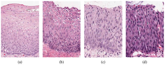
CIN grading label examples. (a) Normal, (b) CIN 1, (c) CIN 2, and (d) CIN 3.

The cervix epithelium is “top-layer” or “surface” tissue which lies over “supporting tissue” called stroma. The basement membrane marks the boundary between stroma and epithelium and may be considered the “bottom” of the epithelium; the opposite side of the epithelium is the apical surface or “top”. As CIN increases in severity, the epithelium has been observed to show an increase in atypical immature cells from bottom to top of the epithelium [4–7]. For example as shown in Fig. 1, atypical immature cells are seen mostly in the bottom third of the epithelium for CIN 1 (Fig. 1b) while those for CIN2 lie in the bottom two thirds of the epithelium (Fig. 1c), In CIN 3, the atypical immature cells comprise the full thickness of the epithelium (Fig. 1d). When these abnormal cells extend beyond the epithelium, grow through the basement membrane and enter into the surrounding tissues and organs, this indicates invasive cancer [5]. In addition to analyzing the progressively increasing quantity of atypical immature cells from bottom to top of the epithelium, identification of nuclear atypia is also important [3]. Nuclear atypia is associated with nuclear enlargement, thereby resulting in different shapes and sizes of the nuclei present within the epithelium. The large number of nuclei and other morphological parameters such as cytoplasm homogeneity, thickness of the nuclear membrane, and the presence of nucleoli contribute to the complexity and difficulty of visually assessing the degree of abnormality. This in turn may contribute to diagnostic grading reproducibility issues and inter- and intra-pathologist variation [6–8]. In previous studies, computer-assisted methods (digital pathology) have been investigated to augment pathologists’ decisions (traditional pathology) for CIN diagnosis [9–15]. Keenan et al. introduced an automated system for CIN degree classification based on an input squamous epithelium region image [10]. The nuclear centers were determined and used as node points for a Delaunay Triangulation mesh. The epithelial region was divided into three equal horizontal compartments, and morphological features were extracted from the triangles within the compartments [10]. Similar methods have been applied toward image analysis of other types of cancer [11]. Guillaud et al. extracted texture features from the epithelium region to estimate the absolute intensity and density levels of the nucleus. Morphological features were also extracted to estimate the nuclear shape, size and boundary irregularities [12,13]. Miranda et al. determined the nuclei in the epithelium using a Watershed segmentation method followed by Delaunay Triangulation to facilitate CIN analysis. This method uniquely assigned CIN grade labels based on triangles formed using the Delaunay Triangulation method, instead of making a CIN grade decision on the whole epithelium image [14].

In another study, CIN classification was performed by analyzing histological features and using a Bayesian belief network classifier. Histological features such as degree of nuclear pleomorphism and number and levels of mitotic figures in the epithelium were examined. These features were linked to a decision node, wherein the decision on CIN grade was made based on conditional probability of the features. However these features were subjective and hence it was difficult to use them in a consistent and reproducible manner for CIN grade classification [15]. One of the recent works applied a decision tree classifier upon morphological features extracted from the nuclei for CIN grade classification [16]. The nuclei were segmented from the epithelium using a K-means clustering and graph-cut segmentation method. The approach used a decision tree for CIN grade classification with empirically determined rules.

Wang et al. developed a comprehensive method for whole slide cervix histology image analysis for CIN grade classification. The method included multi-resolution texture analysis for automated epithelium segmentation, iterative skeletonization to approximate the epithelium medial axis (skeleton), and morphological feature extraction from blocks along orthogonal lines to the skeleton. CIN grade classification of each block was done by an SVM-based classifier using the features extracted from the blocks [17,18]. In a recent pathology study by Marel et al., the epithelium was analyzed in a heterogeneous manner, wherein different regions of the epithelium were shown to exhibit different CIN grades. It was proposed that a particular epithelium with atypical cells could exhibit different CIN grades in different regions of the epithelium along the medial axis, as compared to a homogeneous CIN grade of the epithelium [19]. The research presented in our paper builds on the CIN diagnosis methods proposed by Wang et al. [5] and Marel et al. [19] in the development of a localized, fusion-based approach to provide the capability to address feature and diagnostic variations in different portions of the epithelium and combine those variations into a single diagnostic assessment. The epithelium image analysis approach includes medial axis determination, vertical segment partitioning as medial axis orthogonal cuts, individual vertical segment feature extraction and classification, and image-based classification using a voting scheme fusing the vertical segment CIN grades. The epithelium medial axis is found using a distance transform and bounding box-based technique. The medial axis is divided into 10 equidistant partitions with orthogonal lines to the medial axis used to cut the epithelium region into 10 vertical segments. Features are extracted from each vertical segment for CIN classification. A voting scheme is used to fuse the individual segment CIN grades for image-based epithelium region classification.

For individual segment analysis, we investigated several categories of features, including intensity shading, texture-, correlation- and geometry-based; we used these features as inputs to a classifier for CIN grade analysis. We used a Linear Discriminant Analysis (LDA) classifier to classify the individual segments into the varying grades of CIN. Finally, we used a voting scheme to fuse the class labels of the vertical segments to assign a CIN grade to the whole epithelium. Fig. 2 shows the flowchart of the overall method developed in this study for CIN grade classification.

Fig. 2.

Overview of CIN grade classification method developed in this study.

The rest of the paper is organized as follows. Section 2 presents the methodology used in this research. Section 3 presents the experiments performed. Section 4 contains the experimental results and discussion, while Section 5 provides the conclusions.

2. Methodology

The goal of this research is to classify the squamous epithelium regions from cervix histology images into different grades of CIN. For this study, the squamous epithelium region has been manually segmented by an expert pathologist in collaboration with the National Library of Medicine (NLM). Sixty-two cervix epithelium segmentations were created by the pathologist. Fig. 3 shows a sample cervix histology image and the pathologist manually segmented epithelium region. The segmented epithelium image is shown in Fig. 3b and denoted as I (in RGB format). Let the luminance image of I be denoted as L.

Fig. 3.

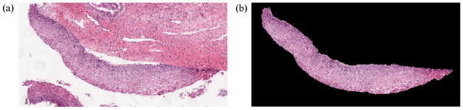
Original image and pathologist segmented image of epithelium. (a) Original image (cervix histology image) and (b) pathologist segmented image I.

Classification of the segmented epithelium images into the various CIN grades was performed using a five-step approach, as outlined in the flowchart in Fig. 2, as follows:

• Step 1: Find the medial axis of the segmented epithelium region (medial axis detection).

• Step 2: Divide the segmented image into 10 vertical segments, orthogonal to the medial axis (vertical segments generation).

• Step 3: Extract features from each of the vertical segments (feature extraction).

• Step 4: Classify each of these segments into one of the CIN grades (classification).

• Step 5: Fuse the CIN grades from each vertical segment to obtain the CIN grade of the whole epithelium for image-based classification.

The following sections present each step in detail.

2.1. Medial axis detection

We used a distance transform and bounding box method to find the medial axis of the epithelium image I. The following steps detail the medial axis detection algorithm developed in this study:

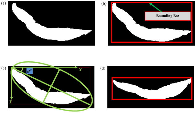
• Step 1: We created a binary mask I^B of the segmented epithelium region shown in Fig. 3b. Note that we cropped the binary mask to contain only the region of the epithelium, as shown in Fig. 4a.

• Step 2: We determined the bounding box of the binary mask I^B, as shown in Fig. 4b. Next, we calculated the Extent ε_{before Rot} of I^B. Extent is defined as the ratio of the non-zero pixels within the bounding box to the total number of pixels within the bounding box.

• Step 3: We calculated the orientation θ^B of the binary mask I^B as the angle (−90° to 90°) between the x-axis and the major axis of the ellipse that has the same second moments as the binary mask. Fig. 4c shows the orientation angle obtained from the Fig. 4b image. We then rotated the binary mask by the negative of the orientation angle −θ^B and denoted the resulting image as ${\mathit{I}}_{\mathit{temp}\_\mathit{rot}}^{\mathit{B}}$. Next, we computed the bounding box for ${\mathit{I}}_{\mathit{temp}\_\mathit{rot}}^{\mathit{B}}$ and also the Extent ε_{after Rot} of ${\mathit{I}}_{\mathit{temp}\_\mathit{rot}}^{\mathit{B}}$ . The bounding box for ${\mathit{I}}_{\mathit{temp}\_\mathit{rot}}^{\mathit{B}}$ is shown in Fig. 4d.

• Step 4: The binary mask ${\mathit{I}}_{\mathit{rot}}^{\mathit{B}}$ for the next steps was selected as follows: if ε_{after Rot} > ε_{before Rot}, then ${\mathit{I}}_{\mathit{rot}}^{\mathit{B}}={\mathit{I}}_{\mathit{temp}\_\mathit{rot}}^{\mathit{B}}$. If ε_{after Rot} < ε_{before Rot}, then ${\mathit{I}}_{\mathit{rot}}^{\mathit{B}}={\mathit{I}}^{\mathit{B}}$. (This logic was motivated by the experimental observation that using a binary mask with a larger Extent provided better estimates of the medial axis.) For the example shown in this paper, ε_{after Rot} = 0.42 and ε_{before Rot} = 0.28. Hence, ${\mathit{I}}_{\mathit{rot}}^{\mathit{B}}={\mathit{I}}_{\mathit{temp}\_\mathit{rot}}^{\mathit{B}}$ as shown in Fig. 4d.

• Step 5: We applied the distance transform to the inverted, rotated binary mask, denoted as $\overline{{\mathit{I}}_{\mathit{rot}}^{\mathit{B}}}$. The Euclidean distance was computed between each pixel, $\overline{{\mathit{I}}_{\mathit{rot}}^{\mathit{B}}}(x,y)$ within $\overline{{\mathit{I}}_{\mathit{rot}}^{\mathit{B}}}$ and the nearest non-zero pixel in $\overline{{\mathit{I}}_{\mathit{rot}}^{\mathit{B}}}$, using the Matlab-based implementation in [20]. The distance transform applied to the mask $\overline{{\mathit{I}}_{\mathit{rot}}^{\mathit{B}}}$ resulted in the distance transform image D as shown in Fig. 5.

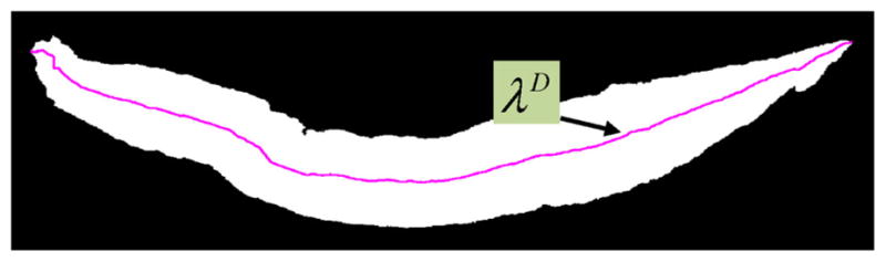
• Step 6: We scanned each column of the distance transform image D for the highest intensity pixel. The coordinates corresponding to the highest intensity pixels obtained in this manner were termed the medial axis coordinates and denoted as the ‘determined’ medial axis λ^D. Thus λ^D is a set of points representing the coordinates of the determined medial axis and is shown in Fig. 6 (magenta color), overlaid on the binary mask ${\mathit{I}}_{\mathit{rot}}^{\mathit{B}}$.

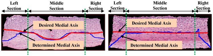
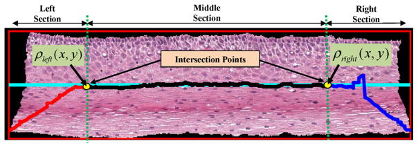
  The determined medial axis λ^D showed medial artifacts for cases when the epithelium images had a somewhat rectangular shape, as shown in Fig. 7. The determined medial axis using the distance transform approach is shown in blue, with the manually marked desired medial axis shown in red. These artifacts occur in the left and right sections of the epithelium as shown in Fig. 7. This is because for the left and right sections, the maximally separated pair of end points (the max for each column) in D is along the corners, as compared to the edges. Therefore the medial axis tends to bend toward the corners as shown in Fig. 7.

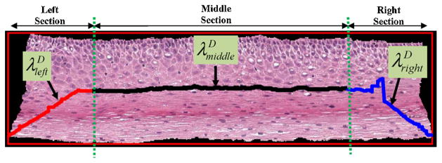
• Step 7: From Fig. 7, it can be observed that the determined medial axis is in approximate agreement with the desired medial axis in the middle/interior section of the epithelium. However, the determined medial axis shows deviations from the desired medial axis in the leftmost 20% and the rightmost 20% of the epithelium. In order to compensate for these end section variations, the determined medial axis λ^D was divided into three pieces, such that ${\lambda }^D=\{{\lambda }_{\mathit{left}}^D,{\lambda }_{\mathit{middle}}^D,{\lambda }_{\mathit{right}}^D\}$ as shown in Fig. 8. Here, ${\lambda }_{\mathit{left}}^D$ (the piece shown in red) represents the leftmost 20% of the medial axis, ${\lambda }_{\mathit{middle}}^D$ (the piece shown in black) represents the middle 60% of the medial axis, and ${\lambda }_{\mathit{right}}^D$ (the piece shown in blue) represents the rightmost 20% of the medial axis.

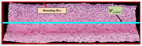
• Step 8: The center line ψ_center of the bounding-box for the epithelium was found and is shown in cyan color in Fig. 9. ψ_center contains the coordinates of the line that divides the bounding box into two halves, top and bottom.

• Step 9: The intersection points, as shown in Fig. 10, were determined. An intersection point was defined as the point where the leftmost (or the rightmost) medial axis piece intersected with the center line (see Fig. 10). The left intersection point was obtained by computing the Euclidean distances between each point (coordinate) of ${\lambda }_{\mathit{left}}^D$ and ψ_center. The point on ${\lambda }_{\mathit{left}}^D$ which had the minimum Euclidean distance to ψ_center was used as the left intersection point and denoted as ρ_left(x, y). If more than two points were found, the point geometrically closer to the middle section (see Fig. 10) was used as the left intersection point. In a similar manner, the right intersection point was determined by obtaining the intersection between the rightmost medial axis piece ${\lambda }_{\mathit{right}}^D$ and the center line ψ_center. The right intersection point was denoted as ρ_right(x, y). These intersection points were used as the points around which the leftmost and the rightmost medial axis pieces were adjusted to create the final medial axis. The intersection points are illustrated in Fig. 10 as yellow dots.

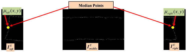
• Step 10: The edge image of the epithelium region was determined. We obtain the edge image I^E by applying a Sobel edge detector on the rotated mask ${\mathit{I}}_{\mathit{rot}}^{\mathit{B}}$. The edge image I^E was created to determine the outer endpoints of the medial axis approximations for the leftmost 20% and rightmost 20% regions. I^E was divided into three parts, as shown in Fig. 11, including: leftmost $20\%({\mathit{I}}_{\mathit{left}}^{\mathit{E}})$, middle $60\%({\mathit{I}}_{\mathit{middle}}^{\mathit{E}})$, and rightmost $20\%({\mathit{I}}_{\mathit{right}}^{\mathit{E}})$. After dividing the edge image into three parts, the median values of edge coordinates of the leftmost edge part ${\mathit{I}}_{\mathit{left}}^{\mathit{E}}$ and rightmost edge part ${\mathit{I}}_{\mathit{right}}^{\mathit{E}}$ were obtained. These median values were denoted as the left median point μ_left(x, y) and the right median point μ_right(x, y), for μ_left(x, y) and ${\mathit{I}}_{\mathit{right}}^{\mathit{E}}$, respectively. The median points are shown as yellow dots in Fig. 11. We observed experimentally that the median points μ_left(x, y) and μ_right(x, y) provide a good estimate of the endpoints of the medial axis pieces ${\lambda }_{\mathit{left}}^D$ and ${\lambda }_{\mathit{right}}^D$, respectively.

• Step 11: The orientation of the leftmost and rightmost medial axis pieces were estimated to rotate those pieces of the medial axis determined. The orientation is defined as the angle by which the leftmost and the rightmost medial axis pieces ( ${\lambda }_{\mathit{left}}^D$ and ${\lambda }_{\mathit{right}}^D$ respectively) are rotated/adjusted to obtain the final medial axis. The determined medial axis pieces were adjusted so as to obtain medial axis pieces that were in close proximity to the desired medial axis. Using the left intersection point ρ_left(x, y) obtained from Step 9 and the left median point μ_left(x, y) from Step 10, the orientation of the leftmost medial axis piece ${\lambda }_{\mathit{left}}^D$ was estimated, and denoted as ${\theta }_{\mathit{left}}^D$. In a similar manner, the orientation of the rightmost medial axis piece ${\lambda }_{\mathit{right}}^D$ was also determined and denoted as ${\theta }_{\mathit{right}}^D$. Note that the orientations of the leftmost and rightmost medial axis pieces obtained in this step were used to adjust the medial axis pieces as described in Step 12.

• Step 12: In this step, the leftmost medial axis piece ${\lambda }_{\mathit{left}}^D$ was rotated by the negative of the orientation $-{\theta }_{\mathit{left}}^D$ to obtain the ‘adjusted’ left-most medial axis piece ${\lambda }_{\mathit{left}}^A$ (note that the superscript ‘A’ refers to the ‘adjusted’ medial axis piece). Similarly the rightmost medial axis piece ${\lambda }_{\mathit{right}}^D$ was rotated by the negative of the orientation $-{\theta }_{\mathit{right}}^D$ to obtain the ‘adjusted’ rightmost medial axis piece ${\lambda }_{\mathit{right}}^A$.

• Step 13: The final medial axis coordinates λ^F were obtained from the determined medial axis coordinates ${\lambda }^D=\{{\lambda }_{\mathit{left}}^D,{\lambda }_{\mathit{middle}}^D,{\lambda }_{\mathit{right}}^D\}$ by replacing ${\lambda }_{\mathit{left}}^D$ and ${\lambda }_{\mathit{right}}^D$ with ${\lambda }_{\mathit{left}}^A$ and ${\lambda }_{\mathit{right}}^A$ respectively. The final medial axis was represented as ${\lambda }^F=\{{\lambda }_{\mathit{left}}^A,{\lambda }_{\mathit{middle}}^D,{\lambda }_{\mathit{right}}^A\}$. Note that the middle medial axis piece ${\lambda }_{\mathit{middle}}^D$ is the same as that of the determined medial axis without any adjustment/rotation.

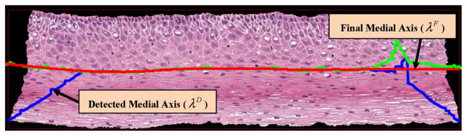
• Step 14: Finally, λ^F was smoothed using a moving average filter with a span of 150 to remove some of the irregularities in λ^F. Fig. 12 shows the determined medial axis (in blue), the final medial axis before smoothing (in green) and the final medial axis after smoothing (in red), overlaid on the epithelium image.

Fig. 4.

Binary mask rotation (Steps 1–4). (a) Original binary mask, I^B (Step 1). (b) Bounding box of I^B (ε_{before Rot} = 0.28) (Step 2). (c) Orientation of the binary mask (θ^B) (Step 3). (d) Rotated binary mask, ${\mathit{I}}_{\mathit{temp}\_\mathit{rot}}^{\mathit{B}}({\epsilon }_{\mathit{after}\_\mathit{Rot}}=0.42)$ (Step 4).

Fig. 5.

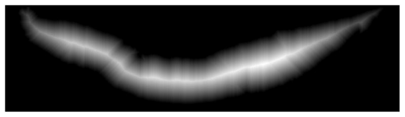
Distance transform image (D) obtained by applying distance transform to the binary epithelium mask image $\overline{{\mathit{I}}_{\mathit{rot}}^{\mathit{B}}}$ (Step 5).

Fig. 6.

Medial axis of the binary mask I^B (Step 6).

Fig. 7.

Determined medial axis vs desired medial axis.

Fig. 8.

Dividing the medial axis into three pieces (Step 7).

Fig. 9.

The center line of the bounding box of the epithelium (Step 8).

Fig. 10.

The intersection points were obtained (Step 9).

Fig. 11.

The edge image was computed and divided into three parts. The endpoints of the medial axis were found using the median of the edge points for the left and right parts (Step 10).

Fig. 12.

Determined medial axis and final medial axis (Step 14).

2.2. Vertical segments creation

Once the final medial axis was determined, the medial axis is divided into 10 equidistant segments. Orthogonal lines are determined at the medial axis points to partition the epithelium into 10 vertical segments. Fig. 13 presents an illustration of the vertical segments to be partitioned within the epithelium.

Fig. 13.

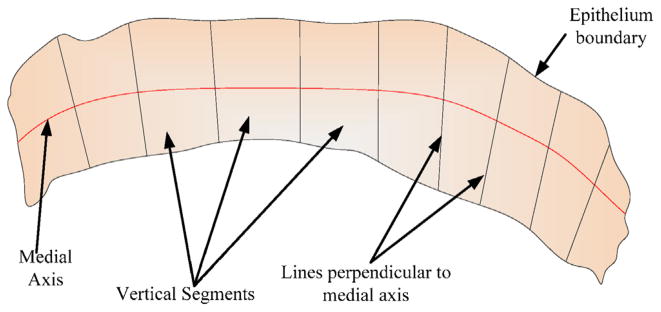
Schematic to show the vertical segments of the epithelium, based on lines perpendicular to the medial axis.

For the vertical segments creation, the final medial axis λ^F was partitioned into 10 equal line pieces such that λ^F = {λ^v₁, λ^v₂, …, λ^v₁₀ } (the superscript ‘v’ denotes the medial axis partitioned into 10 segments, which are used for ‘vertical’ image segments creation). The first line segment λ^v₁ for one of the epithelium images is shown in Fig. 14a. A three-step approach was used for vertical image segments generation:

Fig. 14.

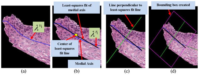
(a)–(d) Steps in obtaining the vertical segments from the epithelium region. (a) First medial axis line segment λ^v₁. (b) The least squares fitted line λ^r₁ obtained from λ^v₁ (Step 1). (c) The perpendicular of λ^r₁ obtained for generating the bounding box (Step 2). (d) The bounding box was generated using the information obtained from Steps (1) and (2) (Step 3).

• Step 1: Each medial axis line segment λ^v₁, λ^v₂, …, λ^v₁₀ was fitted to a linear approximation using a least-squares regression algorithm [21]. An example of the line fitting algorithm is shown in Fig. 14b. Let λ^r₁, λ^r₂, …, λ^r₁₀ denote the fitted medial axis line segments obtained in this manner (note that the superscript ‘r’ denotes regression-fit line). This step was performed to obtain straight line segments to facilitate orthogonal line generation which, in turn, was used for creating the vertical image segments.

• Step 2: Next, the mid-points of each of the fitted medial axis line segments λ^r₁, λ^r₂, …, λ^r₁₀ were obtained; perpendicular lines were drawn from these points, as shown in Fig. 14c, through the top and bottom of the epithelium region.

• Step 3: For each fitted medial axis line segment λ^r₁, λ^r₂, …, λ^r₁₀, we created a bounding box by joining the endpoints of the fitted medial axis of each line segment and the endpoints of the perpendicular lines (obtained from Step 2) to each line segment (illustrated in Fig. 14d). In this manner, for each epithelium image I, 10 bounding boxes (regions) were created.

We used these bounding boxes to partition the epithelium image I (in RGB format) into 10 sections, referred to as vertical segment images and denoted as ${\mathit{I}}_{\mathit{S}}^1,{\mathit{I}}_{\mathit{S}}^2,\dots ,{\mathit{I}}_{\mathit{S}}^{10}$ (in RGB format). Note that depending on the linear approximation of the 10 different partitions for the medial axis, there is the potential that the bounding boxes containing the vertical segment images may overlap. Fig. 15 shows the bounding box and the resulting 10 vertical image segments obtained using this method for one of the sample epithelium images. We then extracted features (given in Table 1) from each of the vertical segment images, and used these features for CIN grade classification, as discussed in the following sections.

Fig. 15.

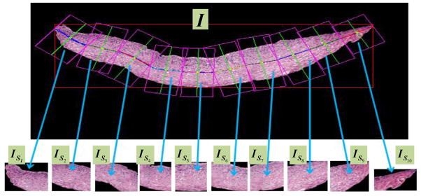
Vertical segment images ( ${\mathit{I}}_{\mathit{S}}^1,{\mathit{I}}_{\mathit{S}}^2,\dots ,{\mathit{I}}_{\mathit{S}}^{10}$) determined from bounding boxes obtained from partitioning the medial axis into 10 line segment approximations.

Table 1.

Feature description.

Feature set	Label	Measure	Description
Texture features	F1	Contrast of segment	Returns a measure of the intensity contrast between a pixel and its neighbor over the whole image
	F2	Energy of segment	Measures the entropy (squared sum of pixel values in the segment)
	F3	Correlation of segment	Returns a measure of how correlated a pixel is to its neighbor over the whole image
	F4	Homogeneity of a segment	Returns a value that measures the closeness of the distribution of pixels in the segment to the segment diagonal
	F5–F6	Contrast of GLCM	Measure of the contrast of the GLCM matrix obtained from the segment
	F7–F8	Correlation of GLCM	Returns a value that measures the closeness of the distribution of elements in the GLCM to the GLCM diagonal
	F9–F10	Energy of GLCM	Returns the sum of squared elements in the GLCM
Triangle features	F11	Average area of triangles	This is the average area of the triangles formed by using Delaunay Triangulation on the nuclei detected
	F12	Std deviation of area of the triangles	This is the standard deviation of the area of the triangles formed by using Delaunay Triangulation on the nuclei detected
	F13	Average edge length	This is the mean of the length of the edges of the triangles formed
	F14	Std deviation of edge length	Standard deviation of the length of the edges of the triangles formed
Profile-based correlation features	F15–F62	Weighted density distribution	Correlation of profile of the segment and WDD function

2.3. Feature extraction

For each vertical segment image, ${\mathit{I}}_{\mathit{S}}^1,{\mathit{I}}_{\mathit{S}}^2,\dots ,{\mathit{I}}_{\mathit{S}}^{10}$, four different types of features were computed, including: (1) texture features, (2) geometry (triangle) features, and (3) profile-based correlation features. Table 1 shows the feature labels and a brief description of each feature, while the following sections elaborate the features. Prior to feature extraction, we convert the RGB images of the vertical segments ( ${\mathit{I}}_{\mathit{S}}^1,{\mathit{I}}_{\mathit{S}}^2,\dots ,{\mathit{I}}_{\mathit{S}}^{10}$) to luminance grayscale images ${\mathit{L}}_{\mathit{S}}^1,{\mathit{L}}_{\mathit{S}}^2,\dots ,{\mathit{L}}_{\mathit{S}}^{10}$. The features are extracted from these luminance images. Let ${\mathit{I}}_{\mathit{S}}^{\mathit{n}}$ denote the RGB image of vertical segment n, where n = 1, 2, …, 10 for the 10 vertical segment images, and let ${\mathit{L}}_{\mathit{S}}^{\mathit{n}}$ denote the corresponding grayscale image. We extracted features for each grayscale vertical segment ${\mathit{L}}_{\mathit{S}}^{\mathit{n}}$.

2.3.1. Texture features

Texture features are usually extracted using structural, spectral or statistical methods [22]. Previous studies on CIN grade classification used texture features such as fractal dimension [12] and measures based on the gray-level co-occurrence matrix (GLCM) [5]. The texture features used in this study include contrast (F1), energy (F2), correlation (F3) and uniformity (F4) of the segmented region, combined with the same statistics (contrast, energy and correlation) obtained from the GLCM of the segment (F5–F10, see Table 1) [23,24]. For calculation of the GLCM matrix, the pixels within a neighborhood of radius 1 were selected, producing the six GLCM related texture measures [5]. This means that the gray level co-occurrence was computed for each pixel ${\mathit{L}}_{\mathit{S}}^{\mathit{n}}(i,j)$ of the vertical image segments over the 3 × 3 neighborhood of ${\mathit{L}}_{\mathit{S}}^{\mathit{n}}(i,j)$ [23].

2.3.2. Geometry (triangle) features

Previous research has shown that the triangles formed by joining the centers of nuclei found using a thresholding technique provide structural information for the squamous epithelium [5,10]. We computed such triangles using the Delaunay Triangulation (DT) algorithm. For a given set of points, DT iteratively selects point triples to become vertices of each new triangle that the algorithm creates. Delaunay Triangulation exhibits the property that no point lies within the circles that are formed by joining the vertices of the triangles [10]. In other words, as shown in Fig. 16c, all the triangles formed using DT are unique and do not contain any points within the triangles. DT uses the coordinates of the points as inputs and provides the vertices of the triangles formed as outputs.

Fig. 16.

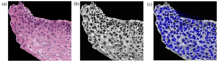
Triangles formed from the vertical segments using Delaunay Triangulation. (a) RGB image of a vertical segment ${\mathit{I}}_{\mathit{S}}^{\mathit{n}}$. (b) Luminance image of a vertical segment ${\mathit{L}}_{\mathit{S}}^{\mathit{n}}$. (c) Triangles created by DT using circle centers detected by CHT.

In the current work, first we used a Circular Hough Transform (CHT)-based method from [25] for nuclei detection (black rounded circular and elliptical objects in the epithelium region) from the vertical segmented images. The outputs of the CHT included: (1) centers of the detected circular or elliptical nuclear objects and (2) distribution of radii (in pixels) of the detected round objects, found within the vertical segments. Note that in elliptical objects, the radius is an estimate of half of the major axis length. For this study, the radius range [min R, max R], where min R = 5 pixels and max R = 15 pixels, to threshold the nuclear objects was empirically determined from the experimental dataset. This radius range was obtained from empirical analysis of the data set for images from each of the CIN grades. The centers of the nuclear objects found using the CHT algorithm were used as points to input into the Matlab-based implementation of the Delaunay Triangulation (DT) method [26].

Fig. 16 shows an example for locating the nuclei using the CHT and then applying the DT algorithm for triangulation (Fig. 16c). The features that were obtained from the triangles include: average area of the triangles (F11), standard deviation of this area (F12), average distance between the edges of the triangles (F13) and standard deviation of this distance (F14) [5,10].

2.3.3. Profile-based correlation features

The third set of features was based on computing profiles of the vertical segments and correlating the profiles with basis functions. In previously published research, profile-based correlation features have been computed for dermatology skin lesion discrimination by correlating the luminance histogram for skin lesion images with a set of Weighted Density Distribution (WDD) basis functions [27]. In our histology image research, we used the method from [27] and applied it to the 1D profiles of the luminance images of the vertical segments ${\mathit{L}}_{\mathit{S}}^{\mathit{n}}$. If R denotes the number of rows and C the number of columns for ${\mathit{L}}_{\mathit{S}}^{\mathit{n}}$, then the profile value of each row, P_S(i) is defined as the average luminance value for each row of pixels inside the epithelium (pixels shown by the red lines in Fig. 17) for each vertical segment luminance image ${\mathit{L}}_{\mathit{S}}^{\mathit{n}}$ as given in Eq. (1).

Fig. 17.

Profile obtained from ${\mathit{L}}_{\mathit{S}}^{\mathit{n}}$ for computing the profile-based correlation features.

$$P_S(i)=\frac{{\sum }_{j=1}^C{L}_S^n(i,j)}{\mathit{numPix}(i)}$$ (1)

for i = 1, 2, …, R. Here numPix(i) denotes the number of pixels that are inside the epithelium for the ith row in the vertical segment luminance image ${\mathit{L}}_{\mathit{S}}^{\mathit{n}}$. Let P_S = {P_S(1), P_S(2), …, P_S(R)} be the sequence of profile values obtained in this manner. We computed correlation features by correlating the profile (P_S) with the WDD functions shown in Fig. 18.

Fig. 18.

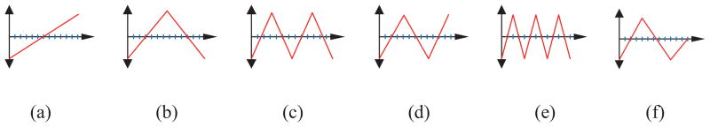
The WDD functions used.

Let T₁ denote the WDD function in Fig. 18(a), T₂ denote the WDD function in Fig. 18(b), and so forth.

The 12 profile-based correlation features were computed as follows.

For the profile P_S, six features q₁, q₂, …, q₆ were computed according to Eq. (2).

$$q_k=\sum _{i=1}^{{\delta }_H}{P}_S(i)T_k(i)$$ (2)

for k = 1, 2, …, 6. We computed six additional features q₇, q₈, …, q₁₂ by correlating the six WDD functions with the sequence of absolute differences between profile sample values as Eq. (3).

$$q_{k+6}=\sum _{i=1}^{{\delta }_H}\mid P_S(i)-P_S(i-1)\mid T_k(i)$$ (3)

for k = 1, 2, …, 6, and P_S(i − 1) = 0 for i = 1.

We calculated a total of 48 profile-based correlation features using the above method for the following four variations of the profile samples (P_S), obtained from the vertical segment under analysis:

1. whole profile, such that P_S = {P_S(1), P_S(2), …, P_S(δ_H)}) (F15–F26);

2. top 1/3rd of the profile such that P_S = {P_S(1), P_S(2), …, P_S(δ_H/3)} (F27–F38);

3. middle 1/3rd of the profile, such that P_S = {P_S(δ_H/3 +1), P_S(δ_H/3 +2), …, P_S(2δ_H/3)} (F39–F50); and,

4. bottom 1/3rd of the profile, such that P_S = {P_S(2δ_H/3 +1), P_S(2δ_H/3 +2), …, P_S(δ_H)} (F51–F62).

As shown above, each 1/3rd of the profile (top to bottom) was analyzed separately along with the whole profile to extract profile-based correlation features for each 1/3rd of the vertical segment images ${\mathit{L}}_{\mathit{S}}^{\mathit{n}}$. Motivation for investigating these features comes from previous work on CIN grade classification highlighting that the epithelium shows structural variation (number of nuclei, and, nuclei-to-cytoplasm ratio) along each 1/3rd (top to bottom) for the different CIN grades [3].

Finally, the feature vector (62 × 1) for each vertical segment image ${\mathit{L}}_{\mathit{S}}^{\mathit{n}}$ was created as:

$$U_{L_S^n}={[\mathrm{F}1,\mathrm{F}2,\mathrm{F}3,\dots ,\mathrm{F}62]}^T$$ (4)

2.4. Classification

As previously stated, 61 cervix histology images with expert pathologist manual segmentations of the squamous epithelium and labeled CIN grades (16 Normal, 13 CIN1, 14 CIN2, and 18 CIN3) were obtained from NLM and examined in this study. The co-authors performed CIN grade labeling of the vertical segments within each image to facilitate classifier training. All experiments score CIN classification results based on the expert pathologist CIN grading of the images. We performed epithelium analysis to classify the 10 individual vertical segments, and then used using a voting scheme for final image classification. For each vertical segment, 62 features were extracted, as discussed in the previous section. These features were used as inputs to a Linear Discriminant Analysis (LDA) classifier for individual vertical segment classification and for image classification.

We used the LIBSVM [28] implementation of the LDA classifier [29]. The LDA method optimizes a linear transformation operator which depends on the ratio of the inter-class variance to the intra-class variance. Optimization of this linear transformation operator was done by maximizing the inter-class variance normalized over intra-class variance, thereby guaranteeing maximum class separability [30,31]. We used the Matlab^® implementation of the method presented in [29].

For image classification, we carried out the following four steps:

• Step 1: Train the classification algorithm (LDA) using a leave-one-image-out approach. The classifier is trained based on the individual vertical segment feature vectors $U_{{\mathit{L}}_{\mathit{S}}^{\mathit{n}}}$ for all but the left-out epithelium image (used as the test image).

• Step 2: Classify each vertical segment of the left-out test image into one of the CIN grades using the LDA classifier.

• Step 3: Assign the test epithelium image to the class (Normal, CIN1, CIN2, CIN3) using a voting scheme. The CIN grade of the test epithelium image was assigned based on whichever class is most frequently assigned to each of the vertical segments for the image (most frequently occurring class assignment for the 10 vertical segments in Step 2). If there is a tie with the most frequently occurring class assignment among the vertical segments, then the epithelium image is assigned to the higher class. For example, if there is a tie between CIN2 and CIN3, then the image would be labeled as CIN3.

• #x02022; Step 4: Repeat Steps 1–3 for all the epithelium images in the experimental data set.

3. Experiments performed

We performed four sets of experiments, which are presented in this section.

3.1. Classification of vertical segment images

For the first set of experiments, all the features extracted from the vertical segment images were used as inputs to train the LDA classifier. Using the leave-one-image out approach (as presented in Step 1 of Section 2.4), the 10 vertical segment images of a test image was assigned CIN grades.

3.2. Fusion of the CIN grades of the vertical segment images

In the second set of experiments, the CIN grades of the vertical segment images obtained from Section 3.1 were fused to obtain the CIN grade of the test epithelium image. Fusion of the CIN grades of the vertical segment images was done using a voting scheme as presented in Step 2 of Section 2.4. We explored three scoring approaches for evaluation of our epithelium image classifications:

• Approach 1 (Exact Class Label): The first approach is exact classification, meaning that if the class label automatically assigned to the test image is the same as the expert class label, then the image is considered to be correctly labeled. Otherwise, the image is considered to be incorrectly labeled.

• Approach 2 (Windowed Class Label): The second scoring approach is a windowed classification scheme. Using this approach, if the predicted CIN grade level for the epithelium image is only one grade off as compared to the actual CIN grade, we considered it as correct classification. For example, if CIN1 was classified as Normal or CIN 2, the result would be considered correct. If CIN1 was classified as CIN3, the result would be considered incorrect.

• Approach 3 (Normal versus CIN): For the third approach, we considered the classification incorrect when a Normal stage was classified as any CIN stage and vice-versa.

3.3. Classification of the whole epithelium

For the third set of experiments, features were extracted from the whole epithelium image, without creating the individual vertical segment images (see Fig. 3b). Features extracted from the whole image were used as inputs to the LDA classifier using the same leave-one-image out approach. This set of experiments was investigated to compare the performance of the fusion-based epithelium classification (Section 3.2) as compared to classifying the epithelium image as a whole. The same scoring approaches as presented in Section 3.2 were used to evaluate the performance of the whole epithelium classification.

3.4. Feature evaluation and selection

Several experiments were performed to evaluate the CIN classification capability of the vertical segment partitioning of the epithelium and the different feature types proposed. First, image-based CIN classification was compared using the voting scheme fusion of the CIN grades found from classifying each vertical segment (Section 2.4) to CIN grades determined based on classifying features computed over the whole image (epithelium) (Section 3.3). As previously stated, we obtained the vertical segment image classifications (CIN grading) using the LDA classifier with a leave-one-image-out approach. We then fused the vertical segment classifications using a voting scheme to obtain the CIN grade of the epithelium image. Similarly, the LDA algorithm was applied in a leave-one-image-out fashion for whole image classification. The following feature combinations were investigated for CIN classification (see Table 1): (1) texture features, (2) triangle features, (3) profile-based correlation features, (4) texture and triangle features, (5) texture and profile-based correlation features, (6) triangle and profile-based correlation features, and (7) texture, triangle, and profile-based correlation features. The fused vertical segment and whole image approaches to image classification were compared using the exact class label, windowed class label, and normal versus CIN scoring methods (Section 3.2).

4. Experimental results and analysis

Based on the experiments described in the previous section, Tables 2 and 3 give the CIN classification results for the vertical segment fusion and whole image approaches, respectively, based on the LDA classifier. Tables 4 and 5 show the confusion matrices for the epithelium image classification results obtained using the vertical segment fusion and whole epithelium region approaches, respectively, using all features (feature combination (7) from the previous section). For the confusion matrices showing the classification results in Tables 4 and 5, adding the diagonal elements of the matrices and dividing by 61 gives the exact class label number of images correct (Approach 1). Combining the diagonal elements of the matrices with the neighboring rows in the same column gives the images correctly classified using the windowed class label method (Approach 2). For Normal versus CIN (Approach 3), any normal image (column 1) that is classified as one of the CIN labels (in column 1, rows 2–4) is an error, and any CIN image that is called a normal image (in columns 2–4, row 1) is an error. The recognition results are presented as the total number of correctly classified divided by the total number of images (61).

Table 2.

LDA classifier results for feature vectors extracted from the vertical segment images and fused to obtain the CIN grade of epithelium. Exact Class Label, Normal versus CIN, and Windowed Class Label results are presented for different feature combinations computed from the vertical segment images.

Features	Exact Class Label	Normal versus CIN	Windowed Class Label
Texture features (F1–F10)	52.3	80.3	96.7
Triangle features (F11–F14)	39.3	82.0	82.0
Profile-based correlation features (F15–F62)	45.9	83.6	88.5
Texture features + triangle features (F1–F10, F11–F14)	54.1	86.9	98.3
Texture features + profile-based correlation features (F1–F10, F15–F62)	54.1	85.2	91.8
Triangle features + profile-based correlation features (F11–F14, F15–F62)	54.1	88.5	90.2
All features (F1–F62)	62.3	88.5	96.7

Table 3.

LDA classifier results for feature vectors extracted from the whole epithelium region to determine the CIN grade. Exact Class Label, Normal versus CIN, and Windowed Class Label results are presented for different feature combinations computed from whole epithelium region.

Features	Exact Class Label	Normal versus CIN	Windowed Class Label
Texture features (F1–F10)	29.5	68.9	73.8
Triangle features (F11–F14)	37.7	73.8	83.6
Profile-based correlation features (F15–F62)	34.4	77.0	85.2
Texture features + triangle features (F1–F10, F11–F14)	54.0	83.6	93.4
Texture features + profile-based correlation features (F1–F10, F15–F62)	26.2	57.8	62.3
Triangle features + profile-based correlation features (F11–F14, F15–F62)	32.8	75.4	82.0
All features (F1–F62)	39.3	78.7	77.0

Table 4.

Confusion matrix for LDA classification results obtained for the vertical segment images fused to obtain the CIN grade using all features.

	Normal	CIN1	CIN2	CIN3
Normal	13	1	1	0
CIN1	2	6	5	0
CIN2	1	6	7	10
CIN3	0	0	1	8

Table 5.

Confusion matrix for LDA classification results obtained for the whole epithelium region to obtain the CIN grade using all features.

	Normal	CIN1	CIN2	CIN3
Normal	9	2	0	2
CIN1	1	5	5	1
CIN2	2	3	5	6
CIN3	4	3	4	9

From Tables 2–5, there are several observations. First, the highest overall classification results were obtained using all features with vertical segment fusion, with accuracies of 62.3% and 88.5%, for the Exact Class Label and Normal versus CIN approaches, respectively. The highest overall Windowed Class Label results were found using the texture and triangle features with vertical segment fusion of 98.3%. Second, vertical segment fusion provided higher overall classification results than the whole epithelium region for the Exact Class Label, Normal versus CIN, and Windowed Class Label approaches, with improvements of 8.3%, 4.9%, and 4.9%, respectively. Third, combining the feature categories for vertical segment fusion and for whole epithelium image classification considerably improved the classification results for all of the scoring approaches (Exact Class Label, Normal versus CIN, Windowed Class Label). None of the feature categories consistently yielded higher classification results. The triangle features from [5] provided the benchmark for comparing the vertical segment fusion and feature development in this research. The triangle features were implemented for whole epithelium region classification in [5]. The classification results for the triangle features, in this study, were higher for the vertical segment fusion approach for the Exact Class Label and Normal versus CIN cases than the whole epithelium region approach, with 1.6% and 8.2% improvements, respectively. For Windowed Class Label classification, the whole epithelium region approach outperformed the vertical segment fusion approach by 1.6%. Third, the confusion matrix results for vertical segment fusion and whole epithelium region classification using all features shown in Tables 4 and 5, respectively, highlight the CIN grades based on the LDA classifier for the Exact Class Label, Normal versus CIN, and Windowed Class Label scoring approaches. The confusion matrices show the similarity between adjacent CIN grades in the LDA classification process, which is representative of the expert pathologist variability for CIN grade assignment of the epithelium [6–8]. Fourth, the results presented in Tables 2–5 appear to indicate that the fusion-based method for CIN grade classification of the epithelium images improves the capability to estimate the epithelium CIN grade compared to analyzing the epithelium as a whole, thus validating the fusion-based approach developed in this study.

For more detailed feature evaluation and selection, we used a SAS^® implementation of Multinomial Logistic Regression (MLR) [32–34]. In general, MLR is used for modeling nominal outcome variables, where the log odds of the outcomes are modeled as a linear combination of the predictor variables. We used the p-values obtained from the MLR output as a metric for feature selection. Specifically, for feature selection, we used the p-values to check the null hypothesis that a particular predictor’s regression coefficient is zero, provided the rest of the predictors in the model are rejected. If a feature has a p-value less than an appropriate alpha (α) value, then the null hypothesis is rejected and the feature is considered to be statistically significant [33–35]. Table 6 shows the features with p-values that satisfy α ≤ 0.05. We examined the reduced feature sets obtained for α ≤ 0.05, α ≤ 0.003, α ≤ 0.002, and α ≤ 0.001. The LDA classification algorithm was applied to the reduced features for the vertical segment fusion and whole epithelium region image approaches to obtain the CIN grade of the epithelium. The Exact Class Label, Normal versus CIN, and Windowed Class Label reduced feature classifications results are presented in Table 7.

Table 6.

Features with corresponding p-values. Only features whose p-values are less than α are shown.

Feature	p-Value	Feature	p-Value	Feature	p-Value	Feature	p-Value	Feature	p-Value
F1	0.0001	F13	0.0039	F23	0.0001	F32	0.0039	F52	0.0047
F2	0.0001	F15	0.0047	F25	0.0036	F34	0.0001	F53	0.0001
F4	0.0001	F16	0.0019	F26	0.0001	F35	0.0002	F54	0.0001
F5	0.0010	F17	0.0033	F27	0.0001	F36	0.0067	F57	0.0021
F7	0.0023	F19	0.0002	F28	0.0001	F37	0.0001	F58	0.0022
F9	0.0001	F20	0.0001	F29	0.0027	F39	0.0007	F59	0.0001
F10	0.0001	F21	0.0001	F30	0.0034	F45	0.0001	F61	0.0001
F11	0.021	F22	0.0007	F31	0.0001	F51	0.0045	F62	0.0011

Table 7.

Vertical segment fusion and whole epithelium image reduced feature vectors for CIN classification results. Exact Class Label, Normal versus CIN, and Windowed Class Label results are presented for features satisfying α ≤ 0.05, α ≤ 0.003, α ≤ 0.002, and α ≤ 0.001 constraints. Results are presented as vertical segment fusion/whole epithelium.

Features	Exact Class Label	Normal versus CIN	Windowed Class Label
α ≤ 0.05 (F1, F2, F4, F5, F7, F9, F10, F11, F13, F15, F16, F17, F19, F20, F21, F22, F23, F25, F26, F27, F28, F29, F30, F31, F32, F34, F35, F36, F37, F39, F45, F51, F52, F53, F54, F57, F58, F59, F61, F62)	65.6%/34.1%	90.2%/77.8	100.0%/77.0%
α ≤ 0.003 (F1, F2, F4, F5, F7, F9, F10, F11, F16, F19, F20, F21, F22, F23, F26, F27, F28, F29, F30, F31, F34, F35, F37, F39, F45, F53, F54, F57, F58, F59, F61, F62)	70.5%/45.9%	90.2%/75.4%	100.0%/82.0%
α ≤ 0.002 (F1, F2, F4, F5, F9, F10, F16, F19, F20, F21, F22, F23, F26, F27, F28, F31, F34, F35, F37, F45, F53, F54, F59, F61, F62)	52.5%/32.8%	85.2%/70.5%	93.4%/68.9%
α ≤ 0.001 (F1, F2, F4, F9, F10, F20, F21, F23, F26, F27, F28, F31, F34, F37, F45, F53, F54, F59, F61)	57.8%/27.9%	86.9%/68.9%	93.4%/78.7%

Based on the results in Tables 2, 3 and 7, we can observe that the reduced feature analysis for the vertical segment fusion of the epithelium images improves the accuracy of CIN grade classification. The highest Exact Class Label classification of 70.5% was found using the features for α ≤ 0.003 (32 total features), which is an improvement of 8.2% over using all features (F1–F62) with vertical segment fusion-based classification. The highest Windowed Class Label classification of 100.0% was obtained using the features for α ≤ 0.05 and α ≤ 0.003, which provides an improvement of 3.3% over using all features (F1–F62) and the texture features (F1–F10) with vertical segment fusion-based classification. The highest Normal versus CIN classification of 90.2% was determined using the features for α ≤ 0.05 and α ≤ 0.003, which provides an improvement of 1.7% over using all features (F1–F62) and the triangle and profile-based correlation features (F11–F14, F15–F62). Considering the reduced feature classification results from Table 7 and the classification results from the feature combinations in Tables 2 and 3, vertical segment fusion provided higher overall classification results than the whole epithelium region for the Exact Class Label, Normal versus CIN, and Windowed Class Label approaches, with improvements of 15.5% (70.5–54.0%), 6.6% (90.2–83.6%), and 6.6% (100.0–93.4%), respectively.

Overall, the Exact Class Label, Normal versus CIN, and Windowed Class Label classification results demonstrate that the vertical segment fusion-based approach provides higher discrimination accuracies for the data set investigated in this study than the whole epithelium feature-based approach. The high classification accuracy obtained using the windowed approach highlights that the nearby classes (Normal/CIN1 or CIN1/CIN2 or CIN2/CIN3) are very similar and therefore difficult to discriminate. It also can be used to explain the intra- and inter-pathologist variation in diagnostic labeling of these images. As compared to the Windowed Class Label (Approach 2) and Normal versus CIN (Approach 3) classification schemes, the Exact Class Label (Approach 1) had lower prediction accuracy. However, the 70.5% accuracy of exact class label prediction using the reduced features is 8.2% higher than the existing benchmark results for automated CIN diagnosis (62.3%) as presented by Keenan et al. [10] and 1.5% higher than the accuracy of the method used by Guillaud et al. (68%) [13]. This suggests that the method developed in this study using the vertical segment analysis and fusion of the vertical segment CIN grades for obtaining the image-based CIN classification yields favorable results to existing methods for automated CIN diagnosis. Even though our method outperformed the existing methods for CIN grade classifications, we note the relatively low classification results for the exact class label scoring approach. Explanatory factors for the low classification scores in this case may include similarity between images of nearby CIN grades such as CIN1 and Normal, CIN1 and CIN2, and CIN2 and CIN3. As shown in the confusion matrices in Table 4, most misclassifications occurred between CIN1 and CIN2 and between CIN2 and CIN3, suggesting that these can be very similar classes. The intra-image variation with the different vertical segments could contribute to variations in CIN grading for the image. It should be noted that the co-author vertical segment CIN labeling used for training the LDA algorithm could have negatively impacted the classification results presented in this study. However, all experiments were performed using the expert pathologist CIN grade labels for the whole image as the classification standard for the different scoring approaches, validating the classification results presented this study. Finally, partitioning the epithelium into vertical segments for local CIN grading provides an alternative context for epithelium (whole image) diagnosis, which can emphasize and integrate local and global assessment in the diagnostic process. The experimental results appear to show that combining the individual vertical segment classifications can improve the overall CIN grading capability for the image versus CIN classification based on global image-based descriptors.

5. Summary and future work

In this study, we developed a framework for automated CIN grade classification of segmented epithelium regions. Our method developed includes medial axis determination, partitioning the epithelium region into vertical segments using the medial axis, individual vertical segment feature extraction, and vertical segment classification and voting-based fusion for final image-based classification We explored texture, triangle, and profile-based correlation features. Experimental results for the proposed vertical segment fusion-based approach achieved classification results as high as 70.5%, 90.2%, and 100.0% for Exact Class Label, Normal versus CIN, and Windowed Class Label scoring approaches, respectively. Classification results also showed that the vertical segment fusion-based approach outperformed the whole epithelium image-based approach, demonstrating the potential for the vertical segment fusion-based approach for enhancing CIN grading of the epithelium.

Future research will explore feature and computational intelligence approaches to improve Exact Class Label classification capability and to examine automation of the epithelium segmentation process in the context of entire slide processing. For such future studies, it is important to include more cervix histology training images to obtain a comprehensive data set for different CIN grades. Automated epithelium segmentation is a computationally intensive and time consuming process, requiring that any algorithm developed for medial axis detection and CIN grade classification needs to be computationally very fast in order to support a reasonable time for automated CIN diagnosis [5,35].

References

- 1.Parkin DM, Bray FI, Devesa SS. Cancer burden in the year 2000 the global picture. Eur J Cancer. 2001;37(Suppl 8):S4–66. doi: 10.1016/s0959-8049(01)00267-2. [DOI] [PubMed] [Google Scholar]
- 2.Jeronimo J, Schiffman M. A tool for collection of region based data from uterine cervix images for correlation of visual and clinical variables related to cervical neoplasia. Proceedings of the 17th IEEE Symposium on Computer-Based Medical Systems; 2004. pp. 558–62. [Google Scholar]
- 3.Kumar V, Abbas A, Fausto N, Aster J. Robbins & Cotran pathologic basis of disease. 8. Philadelphia (PA): Saunders Elsevier; 2009. [Google Scholar]
- 4.He L, Long LR, Antani S, Thoma GR. Computer assisted diagnosis in histopathology. In: Zhao FZ, editor. Sequence and genome analysis: methods and applications. Hong Kong: iConcept Press; 2011. pp. 271–87. [Google Scholar]
- 5.Wang Y, Crookes D, Eldin OS, Wang S, Hamilton P, Diamond J. Assisted diagnosis of cervical intraepithelial neoplasia (CIN) IEEE J Sel Topics Signal Process. 2009;3(1):112–21. [Google Scholar]
- 6.McCluggage WG, et al. Inter- and intra-observer variation in the histopathological reporting of cervical squamous intraepithelial lesions using a modified Bethesda grading system. BJOG: Int J Obstet Gynecol. 1998;105(2): 206–10. doi: 10.1111/j.1471-0528.1998.tb10054.x. [DOI] [PubMed] [Google Scholar]
- 7.Ismail SM, Colclough AB, Dinnen JS, Eakins D, Evans DM, Gradwell E, O’Sullivan JP, Summerell JM, Newcombe R. Reporting cervical intra-epithelial neoplasia (CIN): intra- and interpathologist variation and factors associated with disagreement. Histopathology. 1990;16(4):371–6. doi: 10.1111/j.1365-2559.1990.tb01141.x. [DOI] [PubMed] [Google Scholar]
- 8.Molloy C, Dunton C, Edmonds P, Cunnane MF, Jenkins T. Evaluation of colposcopically directed cervical biopsies yielding a histologic diagnosis of CIN 1, 2. J Lower Genital Tract Dis. 2002;6(2):80–3. doi: 10.1097/00128360-200204000-00003. [DOI] [PubMed] [Google Scholar]
- 9.Soenksen D. Digital pathology at the crossroads of major health care trends: corporate innovation as an engine for change. Arch Pathol Lab Med. 2009;133:555–9. doi: 10.5858/133.4.555. [DOI] [PubMed] [Google Scholar]
- 10.Keenan SJ, Diamond J, McCluggage WG, Bharucha H, Thompson D, Bartels PH, Hamilton PW. An automated machine vision system for the histological grading of cervical intraepithelial neoplasia (CIN) J Pathol. 2000;192(3): 351–62. doi: 10.1002/1096-9896(2000)9999:9999<::AID-PATH708>3.0.CO;2-I. [DOI] [PubMed] [Google Scholar]
- 11.Loménie N, Racoceanu D. Point set morphological filtering and semantic spatial configuration modeling: application to microscopic image and bio-structure analysis. Pattern Recogn. 2012;45(8):2894–911. [Google Scholar]
- 12.Guillaud M, Cox D, Malpica A, Staerkel G, Matisic J, Niekirk DV, Adler-Storthz K, Poulin N, Follen M, MacAulay C. Quantitative histopathological analysis of cervical intra-epithelial neoplasia sections: methodological issues. Cell Oncol. 2004;26:31–43. doi: 10.1155/2004/238769. [DOI] [PMC free article] [PubMed] [Google Scholar]
- 13.Guillaud M, Adler-Storthz K, Malpica A, Staerkel G, Matisic J, Niekirkd DV, Cox D, Poulina N, Follen M, MacAulay C. Subvisual chromatin changes in cervical epithelium measured by texture image analysis and correlated with HPV. Gynecol Oncol. 2005;99:S16–23. doi: 10.1016/j.ygyno.2005.07.037. [DOI] [PubMed] [Google Scholar]
- 14.Miranda GHB, Soares EG, Barrera J, Felipe JC. Method to support diagnosis of cervical intraepithelial neoplasia (CIN) based on structural analysis of histological images. Proceedings of the 25th International Symposium on Computer-Based Medical Systems (CBMS); 2012. pp. 1–6. [Google Scholar]
- 15.Price GJ, Mccluggage WG, Morrison ML, Mcclean G, Venkatraman L, Diamond J, Bharucha H, Montironi R, Bartels PH, Thompson D, Hamilton PW. Computerized diagnostic decision support system for the classification of preinvasive cervical squamous lesions. Hum Pathol. 2003;34(11):1193–203. doi: 10.1016/s0046-8177(03)00421-0. [DOI] [PubMed] [Google Scholar]
- 16.Rahmadwati R, Naghdy G, Ros M, Todd C. Computer aided decision support system for cervical cancer classification. Proceedings of SPIE, Applications of Digital Image Processing XXXV; 2012. pp. 1–13. [Google Scholar]
- 17.Wang Y, Chang SC, Wu LW, Tsai ST, Sun YN. A color-based approach for automated segmentation in tumor tissue classification. Proceedings of the Conference of IEEE Engineering in Medicine and Biology Society; 2007. pp. 6577–80. [DOI] [PubMed] [Google Scholar]
- 18.Wang Y, Turner R, Crookes D, Diamond J, Hamilton P. Investigation of methodologies for the segmentation of squamous epithelium from cervical histological virtual slides. Proceedings of the International Machine Vision and Image Processing Conference; 2007. pp. 83–90. [DOI] [PubMed] [Google Scholar]
- 19.Marel JVD, Quint WGV, Schiffman M, van-de-Sandt MM, Zuna RE, Terence-Dunn S, Smith K, Mathews CA, Gold MA, Walker J, Wentzensen N. Molecular mapping of high-grade cervical intraepithelial neoplasia shows etiological dominance of HPV16. Int J Cancer. 2012;131:E946–53. doi: 10.1002/ijc.27532. http://dx.doi.org/10.1002/ijc.27532. [DOI] [PMC free article] [PubMed] [Google Scholar]
- 20.Maurer CR, Rensheng Q, Raghavan V. A linear time algorithm for computing exact Euclidean distance transforms of binary images in arbitrary dimensions. IEEE Trans Pattern Anal Mach Intell. 2003;25(2):265–70. [Google Scholar]
- 21.Rao CR, Toutenburg H, Fieger A, Heumann C, Nittner T, Scheid S. Linear models: least squares and alternatives. Berlin, Germany: Springer; 1999. [Google Scholar]
- 22.Gonzalez R, Woods R. Digital image processing. 2. Englewood Cliffs (NJ): Prentice-Hall; 2002. [Google Scholar]
- 23.Soh LK, Tsatsoulis C. Texture analysis of SAR sea ice imagery using gray level co-occurrence matrices. IEEE Trans Geosci Remote Sens. 1999;37(2): 780–95. [Google Scholar]
- 24.Stanley RJ, De S, Demner-Fushman D, Antani S, Thoma GR. An image feature-based approach to automatically find images for application to clinical decision support. Comput Med Imaging Graph. 2011;35(5):365–72. doi: 10.1016/j.compmedimag.2010.11.008. [DOI] [PMC free article] [PubMed] [Google Scholar]
- 25.Borovicka J. Technical report. University of Bristol; 2003. Circle detection using hough transforms. Course Project: COMS30121-image processing and computer vision; pp. 1–27. [Google Scholar]
- 26.Preparata FR, Shamos MI. Computational geometry: an introduction. New York: Springer-Verlag; 1985. [Google Scholar]
- 27.Stanley RJ, Stoecker WV, Moss RH. A basis function feature-based approach for skin lesion discrimination in dermatology dermoscopy images. Skin Res Technol. 2008;14(4):425–35. doi: 10.1111/j.1600-0846.2008.00307.x. [DOI] [PMC free article] [PubMed] [Google Scholar]
- 28.Chang CC, Lin CJ. LIBSVM: a library for support vector machines. 2001 Software available at http://www.csie.ntu.edu.tw/~cjlin/libsvm.
- 29.Fan RE, Chen PH, Lin CJ. Working set selection using second order information for training SVM. J Mach Learn Res. 2005;6:1889–918. [Google Scholar]
- 30.Johnson RA, Wichern DW. Applied multivariate statistical analysis. Upper Saddle River (NJ): Prentice Hall; 1988. [Google Scholar]
- 31.Li T, Zhu S, Ogihara M. Using discriminant analysis for multi-class classification: an experimental investigation. Knowl Inf Syst. 2006;10(4):453–72. [Google Scholar]
- 32.Hosmer D, Lemeshow S. Applied logistic regression. 2. New York (NY): John Wiley & Sons, Inc; 2000. [Google Scholar]
- 33.Agresti A. An introduction to categorical data analysis. New York (NY): John Wiley & Sons, Inc; 1996. [Google Scholar]
- 34.Pal M. Multinomial logistic regression-based feature selection for hyperspectral data. Int J Appl Earth Obs Geoinform. 2012;14(1):214–20. [Google Scholar]
- 35.Xue Z, Long RL, Antani S, Neve L, Zhu Y, Thoma GR. A unified set of analysis tools for uterine cervix image segmentation. Comput Med Imaging Graph. 2010;34(8):593–604. doi: 10.1016/j.compmedimag.2010.04.002. [DOI] [PMC free article] [PubMed] [Google Scholar]