New modes of data partitioning based on PARS peak alignment for improved multivariate biomarker/biopattern detection in ¹H-NMR spectroscopic metabolic profiling of urine

Abstract

This paper addresses the possibility of mathematically partition and process urine ¹H-NMR spectra to enhance the efficiency of the subsequent multivariate data analysis in the context of metabolic profiling of a toxicity study. We show that by processing the NMR data with the peak alignment using reduced set mapping (PARS) algorithm and the use of sparse representation of the data results in the information contained in the original NMR data being preserved with retained resolution but free of the problem of peak shifts. We can now describe a method for differential expression analysis of NMR spectra by using prior knowledge, i.e., the onset of dosing, a partitioning not possible to achieve using raw or bucketed data. In addition we also outline a scheme for soft removal of “biological noise” from the aligned data: exhaustive bio-noise subtraction (EBS). The result is a straightforward protocol for detection of peaks that appear as a consequence of the drug response. In other words, it is possible to elucidate peak origin, either from endogenous substances or from the administered drug/biomarkers. The partition of data originating from the normally regulating metabolome can, furthermore, be analyzed free of the superimposed biological noise. The proposed protocol results in enhanced interpretability of the processed data, i.e., a more refined metabolic trace, simplification of detection of consistent biomarkers, and a simplified search for metabolic end products of the administered drug.

Introduction

¹H-NMR data of complex biofluid samples exhibit artifacts, “physicochemical differences,” making interpretation of the multivariate models of the data somewhat problematic. The major data artifacts can be summarized: peak shifts, peak shape distortions (shim problems), and unsuccessful phasing. Other evident problems encountered when analyzing biofluid NMR data are, for example, the inherent bio-variability related to the metabolome of the model system under study such as diurnal variability, individual differences, different hormone levels, and (if applicable), confounded variances related to the event of dosing such as stress, starvation, weight loss, alteration of the gut flora, etc. Finally, there are (variable) co-correlation and large differences in variance magnitude expressed by the peaks in the data, all of which make the search for small variance contributions a difficult task.

Physicochemical differences

Different methods have been proposed to remedy the physicochemical differences, typically by preprocessing the acquired NMR data. The most commonly applied method today is the integration of large segments of the NMR data into “buckets” (Spraul et al., 1994; Holmes et al., 1998) with the aim of collecting unaligned peaks into single buckets. The drawback of the bucketing procedure is the destruction of the high-resolution information by extensive down-sampling of the spectra. As an example: a modest peak detection algorithm indicates that there are approximately 800–1200 peaks present in a 600 MHz NMR spectrum of urine from a healthy rat. When bucketing the spectrum into ∼250 buckets there will, by mathematical necessity, be on average 3–5 peaks (possibly of different origin) per bucket. It is unlikely that these peaks express the same variance pattern, so the resulting integral value will express something different than the true variance contributions. The 3–5 peak number is crude and optimistic since the real situation is much worse – the spectral peaks are not evenly distributed in the NMR spectrum and the used peak picking algorithm does not detect all the minute peaks present. However, the alignment/resolution problem is solved using peak alignment.

Also, the positions of interesting peaks, i.e., peaks occurring as a result of the administered drug or as a consequence of a toxic lesion (potential biomarkers), are usually unknown, making the bucketing procedure integrate peaks of different origin and hence leading to a potentially misleading data analysis result when these buckets are later to be modeled for interesting variance contributions by multivariate methods, i.e., variance mapping methods, principal component analysis (PCA) (Pearson, 1901; Hotelling, 1933; Jackson, 1991) being the most widely used unsupervised multivariate method. PCA decomposes data with descending magnitude of variance as the criterion for mapping the interesting variance patterns of the variables (relative NMR frequency [ppm]). If peaks with varying variances share the same bucket, the peak with the largest variance will dominate the variance pattern, thereby effectively “drowning” smaller peaks. Even worse – spurious variances can accumulate and/or co-correlated and interesting peak variances can be cancelled or blurred. On the other hand, if the spectra were to be modeled in their raw form, the largest expressed variance patterns (loadings) will consist of “shift patterns” (Brown and Stoyanova, 1996; Siuda et al., 1998) expressing the shifts of the largest shifting peaks. Furthermore, added to the shift patterns is information of the inter sample peak shape differences. These shift and shape patterns are of minor interest from a toxicological/metabolic point of view even though it can be stated that the peak shifts express other variables like pH or other ion concentration of the sample (Cloarec et al., 2005).

From a multivariate modeling point of view, there is nothing to be gained from confounding the plethora of NMR peaks reflecting the complex metabolome with the typically univariate parameters mentioned above. If these univariate parameters are of interest, they are best appended to the data in the same way as one would append any other object/sample related study data in the modeling step. The modeling of shift/shape patterns will also deplete the data of useful variance since all variances having a directional component (not orthogonal), with the principal components expressing shift vectors will also, to some extent, be included in the same latent variable, effectively reducing the overall variance in the data regardless of origin. The overall result of using the “bucket” approach or using raw data is that the prospect of modeling or finding small interesting peaks is decreased.

Biological noise

The other major source of unwanted variance has its origin in normal physiological variation or “biological noise.” It is known that that the largest variances of the spectral peaks have their origin in perfectly normal compositional variation of endogenous metabolites that by nature exhibit a large natural time variation. The sources of this normal variation can be traced to (in this study) inter-animal variation (Bollard et al., 2001) and the diurnal cycle (Bollard et al., 2001) of the rat.

There have been quite a number of attempts to remedy the “biological noise” and variance magnitude difference problem, e.g., by imposing different data scaling or transformations such as autoscaling, VAST scaling (Keun et al., 2003), Pareto scaling (Wold et al., 1993), OSC-pretreatment (Andersson et al., 1998), optimized scaling (Karstang and Manne, 1992), etc. The scaling transformations have the aim of transforming the variable variances to have (more) equal numerical magnitudes from a variance-modeling point of view. The desired result is that small variances appear in earlier principal components as they become more pronounced, hopefully making these variables easier to detect. The use of different scaling schemes is the subject of ongoing discussion. The implementation of the different scaling methods and the possible combination of methods is more or less ad lib, making the results from different studies difficult to compare, even though “backscaling” can be performed (Cloarec et al., 2005). Furthermore, scaling schemes such as VAST, OSC, and optimized scaling incorporate prior knowledge (supervised modeling) in the scaling operation, making the quality and validity of the resulting models harder to judge, especially if the following model choice is also supervised with the same classifiers (Y), since the scaled variables are superimposed with class information from the scaling step. The scaling steps based on estimation of variance, e.g., auto- and Pareto scaling, are also founded on the (weak) assumption that the data have an approximately symmetric distribution – a condition not satisfied by the data from a toxicological study.

In this paper we compare three different approaches to process NMR data prior to multivariate data analysis, namely peak alignment using the PARS algorithm (Torgrip et al., 2003; Åberg et al., 2005; Forshed et al., 2005), the traditional “bucketing” scheme and down-sampled raw data. A method is proposed to differentiate interesting sets of metabolites (variables) with respect to causality without loosing the resolution of the NMR data by means of differential expression analysis of the aligned data, a method that can be regarded as unsupervised. Furthermore, a method for removal of “biological noise” by projection/subtraction is outlined. The resulting protocol is a straightforward data partitioning (and projection) where the resulting partitioned datasets are analyzed with an unsupervised method (PCA). The data used to illustrate the processing protocol are 600 MHz ¹H-NMR spectra of rat urine from a time-series study of the metabolic impact of DL-ethionine, a model substance used for induction of hepatic steatosis (fatty liver).

Experimental

Animals and treatments

Thirty-five male rats, 5 per group (Han Wistar, substrain BrlHan:WIST@Mo, approximately 2 months of age at study onset, weight range 220–320 g) were used in the study. Animals were multiple-housed (2 or 3 per cage) during an acclimatization period in the animal house (10 days). During the course of the study, 5 animals/group were housed in individual metabolism cages to allow for the continuous collection of urine. Animals from group 1–3 were dosed by oral gavage in 10 mL/kg PBS with DL-ethionine (DL-2-amino-4-[ethylthio]butyric acid) for 7 days beginning on day 1 and necropsied on day 8, when tissues were taken for pathology. Animals in group 4 were dosed on day 1 and urine was collected until necropsy on day 8. For the animals in groups 1–4, environmental enrichment was provided (crawl balls). Animals in groups 5–7 received a single dose of ethionine on day 1 and were necropsied 24 h after dosing. For details of the animal treatment, see Table 1. The study was performed according to national animal-study regulations.

Table 1.

Animal groups and DL-ethionine dose levels

Group	Dose levels (mg/kg/day)	Dosing period (days)	Necropsy day (day)
G1	0	7	8
G2	20	7	8
G3	80	7	8
G4	800	Single dose	8
G5	0	Single dose	2
G6	80	Single dose	2
G7	800	Single dose	2

Sample collection

Urine samples were collected on ice in 1% (1 mL, w/v) sodium azide prior to dosing (days −5 and −2, one sample/day) and on days 1–7 (0–7 h and 8–24 h, two samples/day [AM/PM]). Urine pH was recorded and the samples were centrifuged at 500 g for 10 min and the supernatant was then retained at −80 °C until analysis with NMR spectroscopy. This scheme resulted in 16 samples/animal for groups 1–4, and 4 samples/animal for groups 5–7.

Although we have not used all the information gathered in this paper, we report the full sampling for completeness. Blood samples for hematology and blood chemistry were taken from the orbital plexus prior to necropsy. Selected organs for histopathology, including liver, kidney, heart, adrenal glands, lungs, pancreas, spleen, stomach, thymus, and testes, were retained at necropsy. Tissue samples were fixed in 10% (w/v) phosphate-buffered formalin and embedded in paraffin wax. Sections were cut and stained with hematoxylin and eosin for light microscopy. Samples from the liver were also freeze-sectioned and stained for fat with Oil Red-O.

¹H-NMR-spectroscopic analysis of urine samples

Aliquots of urine (400 μL) were mixed with 200 μL of 0.2 M phosphate buffer (Na₂HPO₄/NaH₂PO₄, pH=7.4). TSP (3-trimethylsilyl-1-[2,2,3,3,−²H₄] propionate, internal standard) was prepared in deuterium oxide (D₂O) and added to a final concentration of 0.09 mg/ml.

NMR data were acquired on a Bruker DRX-600 spectrometer operating at 600.23 MHz for ¹H observation (Bruker Analytische Messtechnik GmbH, Rheinstetten, Germany). The 4 mm FISEI ¹H–¹³C Z-GRD probe was employed for sample analysis. Spectra were acquired using a standard Bruker NOESY presaturation pulse program (relaxation delay–90°–t₁–90°–t_m–90°–acquire-FID), where t_m was set to 100 ms. The residual water resonances were suppressed, by presaturation during the relaxation and mixing time (t_m). Spectral acquisition parameters used were: 64 free induction decays (FIDs) were collected (64 k data), 12019 Hz spectral width, 2.73 s acquisition time, 4.83 s total pulse recycle delay, at 300 K. The FIDs were zero filled to 64 k and multiplied by an exponential weighting function equivalent to a line broadening of 0.3 Hz prior to Fourier transformation. The study protocol resulted in 336 (of 340 possible) good-quality NMR spectra for further analysis.

Theory

Syntax and definitions

In this paper matrices are expressed as bold capitals, sets and operators as italic capitals, and scalars as italic letters. The term “PCN” is used for PCA dimensionality, where N stands for the actual dimension of the model in question. The term “score(s)” is the projections of the data in question on the principal component “loading” (N). Throughout this paper the term “variable” refers to the ppm annotated NMR spectral intensities. The term “bucketed variable” refers to the center value (ppm) of integrated regions of measured NMR spectral intensities.

We define for a data set of size (R[ows],C[olumns]) a set descriptor, SD, as:

where R is a finite set of objects (rat urine spectrum) , and C is a finite set of variables (relative NMR frequency [ppm]), C={c₁,c₂,...,c_n}, chosen in some way. With this notation the indexing variables R and C can now express a subset of the data. A mapping function is introduced so that operates on a real data set (X), mapping the instances in R and C from X to Z:

We also define a consistency function, C, counting the occurrence of the data mapped in C so that the indexed variables in C are the ones consistently occurring, i.e., not zeros, more than a fraction, α, counted over the accompanying object set (R). For completeness, we also define the full set (all possible instances of objects or/and variables) as . This means that a resulting Z is the subset of objects defined by the set R (the domain) and the subset of variables defined by C (the codomain) occurring in subset R more than a fraction α. Formally:

For the selection of α we refer to the discussion. We also define an additional operator, , mapping the variable space of an SD as

We also define a PCA operator, [T, P]=PCA(X,pcs), performing PCA on the dataset X with the usual output T (scores) and model P (loadings) using pcs principal components. The variable defines a finite set of variances defined by a subset of objects and variables – SD so that it is expressed as . For simplicity, we also define the set of objects (rats) that have not received any drug as UD (undosed and controls) and the set of objects that have received the drug (DL-ethionine) as D (dosed).

Differential expression analysis

Turning our attention to the variable space, there is a possible partitioning of occurrences that can be made since there are at least three possible situations of NMR peaks occurring:

• Peaks occurring in both the UD and the D part of the data

• Peaks only occurring in the UD part of the data

• Peaks only occurring in the D part of the data

The peak-aligned data with sparse representation give us the opportunity to partially differentiate the peak origin by searching the data for the sets reflecting the consistent existence of a peak in the UD set. We define the endogenous set (ENDO) as:

representing the full set of objects with the variables defined as the variables of the UD occurring at least in 75% of the undosed objects. The ENDO peaks are now the consistently occurring peaks stemming from normally occurring endogenous metabolites. Note that these peaks cannot originate from the dosed set, i.e., the ENDO set is free of the problem of being confounded with peaks originating from the dosed substance or its metabolites.

The novel (NOV) partition is now defined as:

i.e., the full set of objects but with the variables who comprise the complement to the variables of the ENDO set. This subset represents all peaks that are not consistently present in the ENDO set but might be consistent in the D set. To sharpen the set, we check the consistency of the NOV set with respect to the D set as:

consisting only of peaks occurring at and after the onset of dosing and occurring in more than 10% of the possible instances in the dosed objects – D. The NOV set will now define the relative spectral NMR frequencies reflecting potential biomarkers (BIOM) not present in the ENDO set and/(or) metabolites originating from the dosed compound and its metabolites (XENO). The NOV set will also contain noise, i.e., noise detected as peaks. Figure 1 depicts the needle vector representation of the found NOV peaks in the data. Note the distribution of the NOV peaks (1494 – peaks detected) covering almost the whole spectral range.

Figure 1.

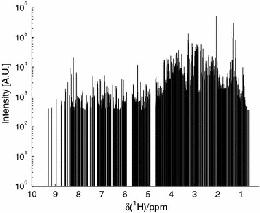
NOV peak distribution (spectra from one rat, G4–D1). Intensity in logarithmic scale for clarity.

We can now focus our “bio-pattern” or “metabolic trace” modeling as well as biomarker detection on the NOV and ENDO sets with less inter-confounding of the sets.

Biological noise removal

Turning to the bio-noise artifact, we must redirect the focus to “patterns” in the data. The variance in the whole NMR data (SD) resulting from a toxicological metabolic profiling study can be partitioned in different ways. One possible way of partitioning is the following:

or formally

The ENDO-related variance can again be partitioned into:

where the biological noise (BIN) variance is primarily the result of normal biological activity, as explained in the introduction. This bio-noise reflects the variance in the metabolome stemming from normal (healthy) time variability and individual differences and is of minor interest from a toxicological metabolic profiling perspective; however, this variance blurs the data analysis by its sheer magnitude. The biologically interesting variance (BIV) is the portion of variance associated with distinguishing the toxicity or lesion in the ENDO expressed by the variables that occur naturally in the rat metabolome (potential biomarkers or “bio-patterns”).

The total variance of the SD can now be expressed by the sum of the following contributions:

or as in the Venn diagram in figure 2.

Figure 2.

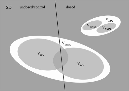
Venn diagram of the data variance partitioning.

The goal of the multivariate data analysis is now to highlight the interesting variables or variable patterns in the BIV and NOV sets, now without the sets being obscured by inter-set variance contributions.

The NOV set has already been defined and can safely be removed from the SD as a set of defined ppm variables and at the same time we rename the SD to ENDO since we have partitioned the SD into two new datasets. In variance terms:

The BIN in the data under consideration can be removed if we can model this fraction of the variance and then subtract the uninteresting variance from the data, i.e., find a way to make V_BIN→ 0.

To express the BIN part (bio-variability/biological noise) of the data, we must understand that this is a variable “pattern” describing what is normally expressed in the metabolome of the rat cohort under study. To express this part of the variance in the ENDO set we have to express the UD subset as a model and deplete the ENDO partition of the variance described by this model.

Now, one naïve way of exhaustively depleting the ENDO of BIN is to model the UD part of the ENDO data, i.e., and

We now define X_E as and project this set onto the model followed by subtraction, i.e.,

This projection/subtraction can be viewed as defining the sub-space of X_E in terms of P, reflecting the bio-noise (of the UD set) and collapsing this subspace on the null-space of X_E. This projection/subtraction effectively cancels the variance in the whole set (X_E) that can be modeled using the UD subset and leaves the new X_BIV matrix depleted of variance related to natural processes and focused on variability related to non-normal metabolic events, i.e., in this case – the onset of toxicity. We have coined this set projection/subtraction exhaustive bio-noise subtraction (EBS). It should also be noted that if the onset of dosing inflicts bionoise with another variance structure than in the undosed set, this couldn’t be modeled with the EBS. After performing EBS, we now end up with data (X_BIV) expressing the following variance pattern:

We now have the overall result of being able to partition the data into at least two new sets of interest, the BIV set, containing the normal metabolite variances cleaned from biological noise, and the NOV set, containing variances from the biomarkers and the excreted/metabolized drug. The full data partitioning/projection can now be summarized by means of a flowchart, figure 3.

Figure 3.

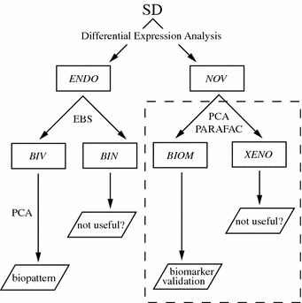
Flowchart of the data partitioning according to variance contributions.

Post processing of NMR spectral data

The resulting FT-transformed NMR spectra were automatically phased, baseline-corrected, and referenced, TSP (δ0.0), using in-house software (PhaseCore^©–AstraZeneca) written for Matlab (Matlab, 2002).

For the comparison of data processing, the effective data range was (0.2–10) ppm. The (4.7–4.9) ppm and (5.7–5.9) ppm spectral regions were excluded from analysis (water and urea respectively). The spectra were normalized to constant sum. The “raw” data are the full (∼64 k) set down-sampled once, i.e., every other datum is removed for computational speed. The bucketing was performed with 0.04 ppm segments with post-summation of the 2.66 and 2.74 ppm buckets into the 2.70 ppm and the 2.50 and 2.58 ppm into the 2.54 ppm bucket for gross correction of the citrate resonances. The bucketing procedure resulted in a compression from ∼64 k data/sample to 205 buckets/sample.

All data analysis was carried out using Matlab. The algorithm invoked for the PCA analysis was the standard SVD (Golub and van Loan, 1989) as implemented in Matlab (T = US, P=V). Peak alignment of the data was performed using the PARS algorithm with an in-house software package written for Matlab (WarpCore^©–AstraZeneca). The NMR data were transformed, aligned, and analyzed using the needle-vector/sparse peak representation, see figure 4, to a resolution of 0.001 ppm in the range of (0.2–10) ppm resulting in 9800 datum/NMR spectrum (336×9800 for the full dataset), which is considered to be the practical working resolution of the used NMR spectrometer.

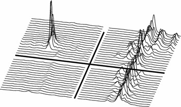
Figure 4.

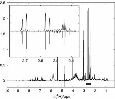
NMR data. Inlay depicts the citrate region with the corresponding sparse/needle vector representation as negative peaks.

All other partitioning, bucketing, wrapping, and plotting software was developed in-house for Matlab. All processed partitions are analyzed by PCA using the covariance matrix, with the exception of the introductory comparison, which uses the mean of the UD set as anchor except for the BIV model, which uses the EBS–PCA model as a multiplicative model of the baseline (the mean of the UD set is the first principal component in the EBS model).

Results

The result is not intended to represent an in-depth analysis of pathways or lesions but is an attempt to express the quality and interpretability of the differently treated data in a metabolic profiling/biomarker detection context.

Pathology of the animal study

DL-ethionine induced the toxicological effects reported in the literature (Farber, 1967; Glaser and Mager, 1974). Animals in group 3 lost approximately 10% of their body weight after dosing with 80 mg/kg/day for 3 days and were euthanised due to ethical reasons (resulting in 140 control and 196 dosed urine samples for data analysis). In brief, periportal hepatic steatosis was observed in animals in groups 3, 6, and 7. In addition, slight liver cell necrosis was also observed in animals of these groups. Furthermore, all 5 rats from group 7 showed tubular degeneration in the kidneys and tubular regeneration was observed in animals treated with a single high dose of ethionine, necropsied at day 8 (group 4). No other organ toxicities were observed.

Introductory data comparison by PCA

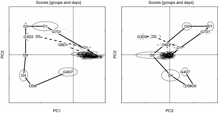
In order to compare methods, we have separately analyzed the raw, bucketed, and peak aligned NMR data. PCA of these three “native” (centered) sets reveals the following data structure, where relevant score and loading plots are depicted in figures 5–13. All three data sets exhibit a distinct time-/dose-dependent score trajectory expressing the metabolic trace of the drug impact. Interestingly, there seem to be two phenomena occurring (tracked by G4) – approximated with one arrow (from center to G4-D1) as the result of administering the drug followed by a transition (G4-D1 to G4-D4), and a third (G4-D4 to G4-D7), which seem to express the behavior of the recovery group (G4).

Figure 6.

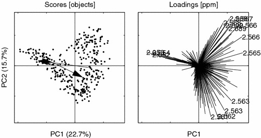
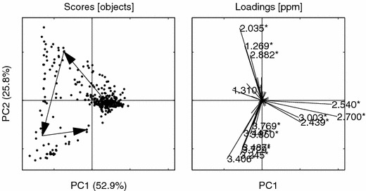
PCs 1 vs. 2 for the raw data, scores on the left pane and loadings on the right. The fifteen largest (Mahalanobis sense) variable loadings are annotated with their corresponding ppm values. (2.567, 2.566, 2.568, 2.053, 2.566, 2.562, 2.563, 2.561, 2.054, 2.052, 2.568, 2.563, 2.690, 2.689, 2.565).

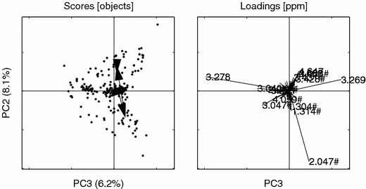
Figure 7.

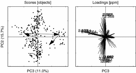
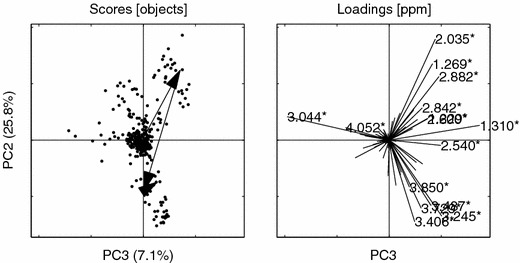
PCs 3 vs. 2 for the raw data. Loading ppm (2.053, 2.054, 2.052, 2.562, 2.561, 2.561, 2.563, 2.568, 2.567, 2.054, 2.568, 2.052, 2.560, 2.682, 2.682). Other details as in figure 6.

Figure 8.

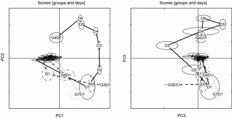
Scores trace for bucketed data. Details as in figure 5.

Figure 9.

PCs 1 vs. 2 for the bucketed data. Asterisks (*) indicate buckets that are confounded with the peaks from the NOV set, see figure 1. Loading ppm (2.700^*, 2.540^*, 2.035^*, 3.406^*, 3.245^*, 1.269^*, 3.729^*, 2.439^*, 3.487^*, 3.003^*, 2.882^*, 3.447^*, 1.310^*, 3.850^*, 3.769^*). Other details as in figure 6.

Figure 10.

PCs 3 vs. 2 for the bucketed data. Asterisks (*) indicate buckets that are confounded with the peaks from the NOV set, see figure 1. Loading ppm (2.035^*, 3.044^*, 1.310^*, 3.245^*, 1.269^*, 3.406^*, 2.882^*, 3.487^*, 3.729^*, 2.540^*, 3.850^*, 4.052^*, 2.842^*, 1.229^*, 2.600^*). Other details as in figure 6.

Figure 11.

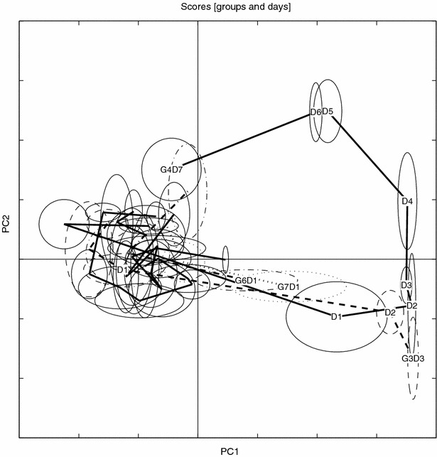
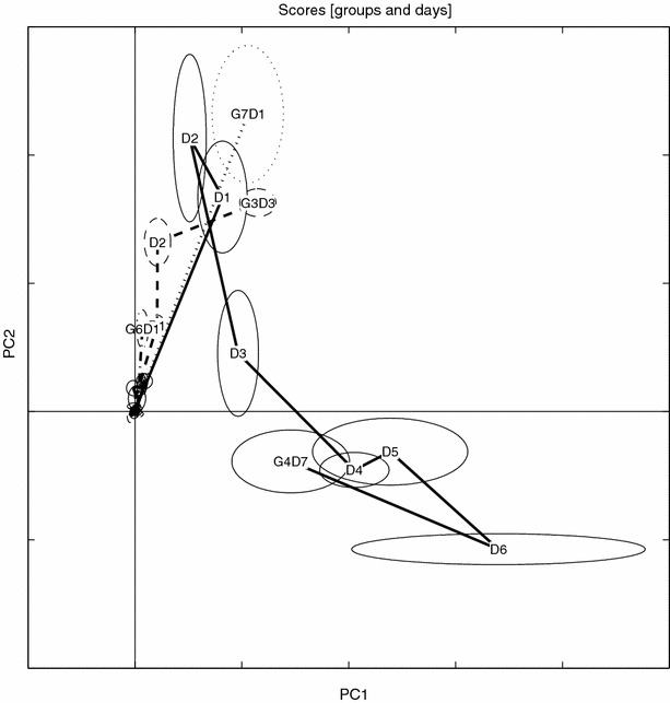
Scores trace for aligned data. Details as in figure 5.

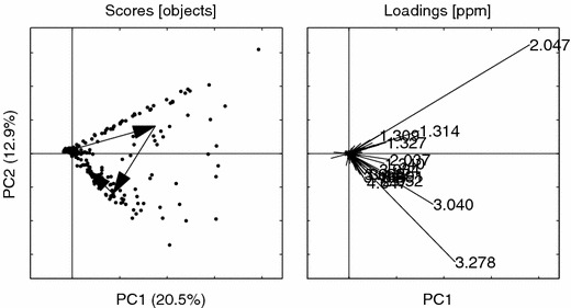
Figure 12.

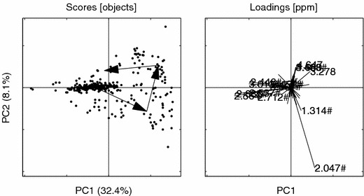
PCs 1 vs. 2 for the aligned data. Hashes (#) indicate loadings that are common with the bucket model. Loading ppm (2.047^#, 2.564, 2.685^#, 3.013^#, 2.537^#, 2.446^#, 2.712^#, 3.278, 1.314^#, 4.647, 4.660, 3.001^#, 3.488^#, 2.457^#, 2.434^#). Other details as in figure 6.

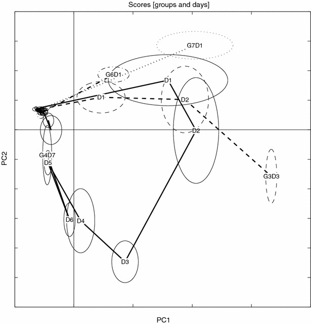
Figure 5.

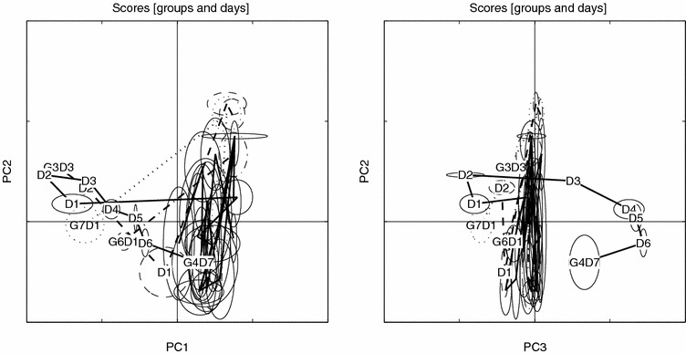
Scores trace for raw data, PC1 vs. PC2 and PC3 vs. PC2, visualized with small sample statistics. The score ellipses for each group (both AM and PM samples) are defined by the median (center) and ±MAD (major and minor axes) in score space. Day is indicated by D and group (last day) by G.

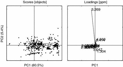
Figure 13.

PCs 3 vs. 2 for the aligned data. Hashes (#) indicate loadings that are common with the bucket model. Loading ppm (3.278, 2.047^#, 3.269, 3.040^#, 3.047^#, 4.647, 1.314^#, 3.488^#, 4.660, 2.052^#, 4.059^#, 3.291, 1.304^#, 3.431^#, 3.428^#). Other details as in figure 6.

Differential expression analysis

From this section on, all models are based on different partitions of aligned data as explained in the post-processing/theory section.

The NOV partition

The differential expression analysis detected 1494 NOV peaks. To ascertain the origin of the NOV peaks (see figure 1), we can now model the NOV set with, e.g., PCA, or a PARAFAC (Harshman, 1970; Bro, 1997) model of the matching time resolved part. The results of the NOV–PCA model can be seen in figures 14 and 15, where we can identify two different phenomena – one loading in the same direction as 2.047 ppm (the dosing) and one related to the 3.278 ppm peak. The peaks localized between these seem to be involved with the transition between the two phenomena detected. Note the few loading variables indicating down regulation – just as expected.

Figure 14.

Scores trace for NOV data. Details as in figure 5.

Figure 15.

PCs 1 vs. 2 for the NOV data. Loading ppm (2.047, 3.278, 3.040, 1.314, 2.052, 3.291, 4.647, 2.037, 1.327, 1.309, 1.340, 3.934, 3.488, 3.447, 3.033). Other details as in figure 6.

The ENDO partition

For completeness a PCA model of the ENDO partition is depicted in figures 16 and 17. This is the structure of the data using only peaks that occur consistently in the whole UD set, i.e., a PCA model of endogenous compounds with the biological noise still present in the ENDO data.

Figure 16.

Scores trace for ENDO data. Details as in figure 5.

Figure 17.

PCs 1 vs. 2 for the ENDO data. Loading ppm. (3.269, 2.564, 2.685, 2.537, 3.013, 2.446, 2.712, 3.001, 2.457, 1.304, 4.660, 2.434, 3.024, 3.414, 3.047). Other details as in figure 6.

Exhaustive bio-noise subtraction (EBS) – the BIV partition

The differential expression analysis detected 324 ENDO peaks. A PCA model of the BIV (EBS treated ENDO set) partition is depicted in figures 18 and 19.

Figure 18.

Scores trace for BIV data. Details as in figure 5.

Figure 19.

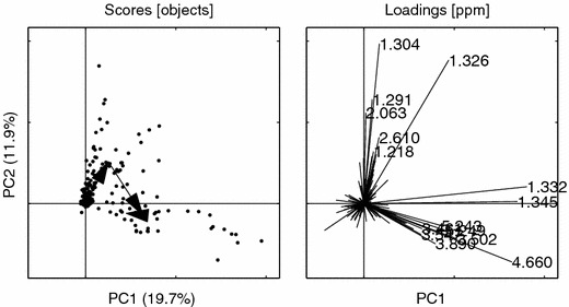
PCs 1 vs. 2 for the BIV set. Loading ppm (1.326, 1.304, 1.332, 4.660, 1.345, 1.291, 2.063, 3.502, 5.249, 3.890, 5.243, 2.610, 3.547, 3.461, 1.218). Other details as in figure 6.

To validate the BIV set, we also modeled the combined groups G1 (control) and G2 (low dose) that, according to pathology, did not show any signs of steatosis, see figure 20.

Figure 20.

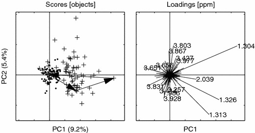
PCs 1 vs. 2 for the BIV set of groups G1 and G2. Undosed (·), Dosed(+). Loading ppm (1.304, 1.313, 1.326, 3.803, 3.928, 3.867, 3.651, 3.831, 2.039, 1.986, 3.414, 3.427, 3.977, 3.656, 3.257). Other details as in figure 6.

In this plot we can clearly see a dose-dependent behavior of the (low-) dosed animals even though pathology could not report any toxic lesion indicating the possibility of an early indication of steatosis.

Discussion

Peak alignment

The conversion from digitized raw spectra to needle vector representation is straightforward since a peak integral is (up to a noise factor) proportional to the peak height. To address the statement that alignment destroys information about the ion content in the sample (Cloarec et al., 2005) the following argument may be set forth: On the contrary, chemometrics is very concerned about un-confounding. Orthogonality, which is a key concept in chemometrics, is the opposite to the proposed modeling of full data. The alignment procedure can be regarded as a means of un-confounding the data from shift information. If the shift information found is of interest, the alignment procedure reports the shift that is applied to each peak in the spectrum, making it possible to either append the applied shifts to the data or analyze these shift data separately. This way of handling and analyzing the shifts is much more efficient than having the peaks confounded with the shift phenomena since the shifts express something different than the peak intensities. It should be emphasized that all relative NMR frequency values reported for the aligned data are at the resolution R=0.001 ppm as opposed to the bucketed data, where R=0.04 ppm. Also of note is the fact that the peak-tracking algorithm used is set to trace the most prominent peaks. A more realistic peak count for this data is approx. 5–6000 peaks/sample (results not shown).

Introductory comparison of the data by PCA

As can be seen we do not report any cross-validation (CV) results from modeling the data. This is superfluous in this case since we only are interested in biomarker detection, i.e., a covariance map of the data in question. It is also dangerous to use the (blocked) CV when there are comparably few samples spanning the interesting metabolic trajectory, i.e., the chance of an important sample being left out is high since we are not sampling from a uniform distribution. In addition, the final models are not used for prediction, making the CV analysis uninformative.

The conclusion of the introductory comparison is that the three different methods result in a time-/dose-dependent trajectory. A PCA of the raw data results in a model that (as expected) mostly reflects the shifting of the citrate peaks. In the bucketed model, although displaying a nice trajectory, the indicated important loading variables are “contaminated” with peaks originating from the NOV partition, calling into question the validity of the indicated peaks. As for the aligned data, the model reflects approximately the same variance pattern and important relative NMR frequencies as the bucketed model, indicating a successful alignment.

Differential expression analysis – selection of

The only user-defined parameter in the differential expression analysis is the peak consistency parameter alpha. Given that we want to detect the ENDO partition with some consistency and given that the alignment procedure can fail for some peaks, a value of 75% is reasonable and sufficient (lower bound). For the “cleanup” of the NOV partition, some prior knowledge of half-life of the dosed compound is beneficial. Assuming an approximate half-life of 12 h, we should be able to track the compound for at least 2 days, making the window of detection at least 4 samples out of 16 possible (25%). In view of this a threshold of 10% is reasonable. The selection is not crucial if the choices are made to incorporate more peaks. The subsequent data analysis (PCA) and additional confirmation in the raw spectra will effectively screen out any spurious NMR variables.

The NOV partition

The fact that the NOV peaks are in abundance and distributed over the whole spectral range in this case questions the use of the bucketing tactic since removal/deletion or replacement (Ebbels et al., 2002) of all the affected buckets would result in virtually no data left to model. In other words, the probability that any bucket segment will be confounded with at least one NOV peak is high. In this study 95% (1494 NOV peaks indicated) of the buckets are confounded with peaks from the NOV set, leaving only 11 buckets un-confounded. This makes the PCA analysis of bucketed data self-validating since it is difficult a priori to remove all peaks originating from the administered drug or its metabolites or any other peaks co-varying with the administration of the dosed compound that are not biomarkers.

Even though the NOV set holds out the promise of detecting “biomarkers” (as new peaks, correlating with the pathology), we have not further elucidated the partitioning (BIOM/XENO) and modeling of the NOV set in this paper since it ultimately requires detection and deletion of the administered compound and its metabolite peaks from the NOV data. It should be stated that this deletion/partitioning step is now a much simpler process since the NOV set has been defined/extracted, thereby becoming open to biomarker detection less affected by other variances. The PCA model of the NOV set also reveals a clustering in loading directions, indicating groups of peaks with different pharmacokinetics, which is a very useful phenomenon when it comes to ascertaining the peak origin. There is now also the possibility of modeling the NOV data with PARAFAC or Tucker types of models since parts of the data (G1, G2 & G4) can be ordered in a tensor with time as one dimension (rat×time×NMR) enabling resolution of time dependent phenomena, possibly revealing the pharmacokinetics of the different events (Connor et al., 2004; Dyrby et al., 2005). In this case any clustering or relevant time-trajectory of the NOV partition indicates loadings with peaks related to either the XENO or the BIOM set of peaks, opening up the way for further model-based assignment of peaks into the XENO or BIOM set.

The power of the PCA–NOV model can be visualized by plotting some indicated spectral areas over time, figures 21 and 22, and by plotting the mean value of the spectral peaks over time, figure 23. The plots reveal peaks that clearly conform to the event of dosing.

Figure 21.

Timeplot of spectral segments (width=0.04 ppm) of peaks indicated by the NOV model, see figure 15. Left segment center 2.047 ppm, right segment center 3.278 ppm. Upper half is dosed (G4), lower half is control animal (G1). Time points from bottom up in each half (−5, −2, 1, 2, 3, 4, 5, 6, 7), −5 and −2 one sample/day, 1–7 two samples/day.

Figure 22.

Timeplot of segments/peaks indicated by the NOV model, see figure 15. Left segment center 3.040 ppm, right segment center 1.314 ppm. Other details as in figure 21.

Figure 23.

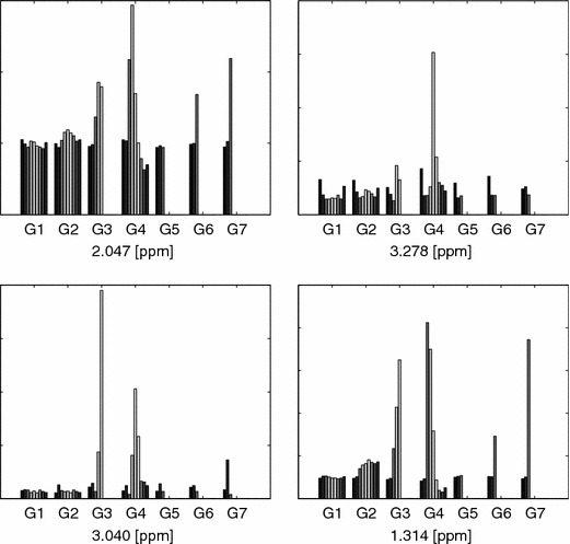
Barplots of the four largest variances indicated by the NOV model, see figure 15. The mean of the intensity for the respective relative NMR frequency for all the rats in a group is pooled into one bar. Time points from left to right (−5, −2, 1, 2, 3, 4, 5, 6, 7) for all groups (G1–7).

Biological noise removal (EBS) and the BIV partition

When comparing the models of the ENDO and the BIV sets, it is obvious that the impact of the peaks has changed. EBS effectively reweighs the variables to reflect variance patterns not easily detected in the UD set, putting emphasis on the changes occurring as a consequence of the transition between UD and D, i.e., we get an immediate focus on the variables exhibiting a variance pattern that cannot be accounted for as being “normal” variation.

One issue with EBS is the number of PCs to use for this projection/subtraction. From a data-modeling point of view, we would like all the biological noise to be canceled, which calls for a relatively high number of PCs; in addition, the variance in the UD subset of the data cannot be of interest for the subsequent data analysis if the toxic event is the focus of the analysis. In other words, there can be no variance of interest from a toxicological perspective in the control set. If there is any variance related to latent biological noise in the data part reflecting the dosing (D), this portion of variance can safely be removed since it is based on the natural bio-variability of the studied rats. This makes the choice of model dimensionality straightforward: one must at least extract as many PCs as there are latent phenomena in the UD set. If one extracts too many, this is of minor concern since the “loading patterns” associated with these PCs will not be present (in large magnitude) in the full data, i.e., these loadings will model bio-noise at an individual rat level, effectively screening out “outlying” individual rats. Hence the overall data will not be affected by the choice of model dimensionality as long as the number is not too small. For this work we have chosen pcs=9, which might be considered a large number; however since there are (7×5×2)×2=140 urine spectra in the UD set expressing partially unique bio-variability patterns, the figure is reasonable. The sensitivity of the choice of PCs can be made clear by, for instance, plotting the explained variance (as sums of squares) for different choices of PCs, see figure 24.

Figure 24.

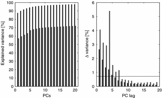
Left pane: explained variance of the EBS correction of the ENDO set, left bars= UD, right bars=UD+D(Ω). Right pane: delta explained variance between PCs. Horizontal line in right pane is at 1/140 – the expected variance contribution of one sample with random variables.

The plot reveals a smooth asymptotic behavior of the modeling power of each PC, indicating that later PCs are explaining noise or individual rats. The figure also shows that approximately 70% of the variance of the ENDO set can be traced to the bio-variability expressed by the UD partition, leaving 30% of the variance explaining changes in the metabolome that cannot be accounted for by the natural variability.

The spectral areas indicated by four selected loading variables from the BIV model, figure 19, are depicted in figures 25 and 26.

Figure 25.

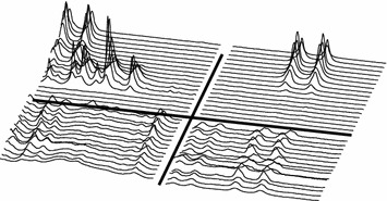
Timeplot of segments/peaks indicated by the BIV model, see figure 19. Left segment center 1.304 ppm, right segment center 3.502 ppm. Lower half is control animal (×10) (G1), other details as in figure 21.

Figure 26.

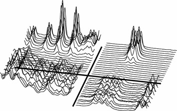
Timeplot of segments/peaks indicated by the BIV model, see figure 19. Left segment center 4.660 ppm, right segment center 5.243 ppm. Lower half is control animal (×10) (G1), other details as in figure 21.

To further visualize the findings in the BIV set, we can plot the time trajectory for the same peaks, see figure 27.

Figure 27.

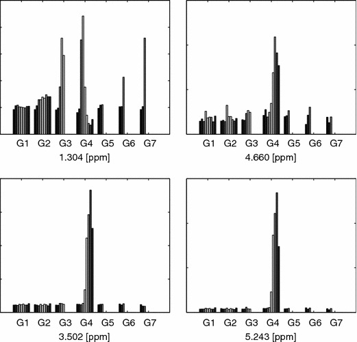
Barplots of BIV model, see figure 19. Details as in figure 23.

The findings for the indicated BIV–G1G2 model can be further validated by analyzing the mean intensities for the full time evolution of some of the peaks of interest for all rats and all groups in the study, see figure 28.

Figure 28.

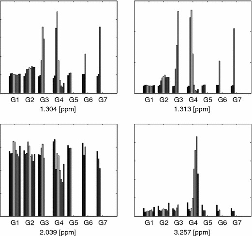
Barplots of BIV–G1G2 model, see figure 20. Details as in figure 23.

It is also noteworthy how the EBS correction brings the distinct “triangular” metabolic trajectory back from the processed ENDO set. It is clear that the ENDO set is heavily “contaminated” with large variances originating from the normally regulating rat metabolome, whereas the BIV set again exhibits the dose trajectory similar to the one seen in the un-processed data, compare figures 16–17 with 18–19. In this study the EBS has been used in a naïve way. A more powerful way of performing EBS is to build a “database” of control and pair-fed animals, making the EBS correction a global correction. Another interesting feature of the EBS projection is that it can be performed on three- or higher way tensors (e.g., MS/MS or LC/MS data) by using high-order decomposition methods such as Tucker or PARAFAC with, in essence, the same philosophical approach.

Concluding remarks

In this paper we indicate methods for circumventing what has been addressed as problems in the multivariate analysis of NMR data in a metabolic profiling context namely unaligned peaks, biological noise, detection of consistent peaks, and the segment integration issue.

We indicate that differential expression analysis of peak aligned NMR data in the context of metabolic profiling is possible. We show that, with proper understanding of the confounding factors, these factors can be removed and/or differentiated into different data sets and the processed data can be further analyzed, revealing the metabolites reflecting the biological system under study. This analysis can, furthermore, be done using unsupervised methods resulting in unbiased modeling. We have also shown that it is possible to remove variance related to normal bio-variability from parts of the data.

Furthermore, the proposed analysis scheme is made with the practical instrument resolution, facilitating the search for indicative chemical shifts and hereby also the assignment of peaks (chemical structure) reflecting the changes in the metabolome. The indicated possibility of finding relevant NMR peaks at this resolution opens up interesting possibilities.

We have shown that the information revealed by the PCA models of the different data partitions differs from the models of bucketed or raw-data. The models of raw data are complex due to the included modeling of shifting peaks and peak shape differences. We have also shown that models of “bucketed” data are affected by a multitude of peaks/variances that cannot be accounted for by the normally regulating metabolome or adjusted for by simply removing/replacing a few “buckets.”

The PARS alignment and the needle/sparse vector representation combined with differential expression analysis and the further partitioning combined with exhaustive bionoise subtraction (EBS) constitutes a straightforward data-processing scheme which unlocks more information at a resolution not hitherto achieved.

References

- Andersson P.M., Sjöström M., Lundstedt T. Preprocessing peptide sequences for multivariate sequence-property analysis. Chemom. Intell. Lab. Syst. 1998;42:41–50. doi: 10.1016/S0169-7439(98)00062-8. [DOI] [Google Scholar]
- Bollard M.E., Holmes E., Lindon J.C., Mitchell S.C., Branstetter D., Zhang W., Nicholson J.K. Investigations into biochemical changes due to diurnal variation and Estrus cycle in female rats using high-resolution 1H-NMR spectroscopy of urine and pattern recognition. Anal. Biochem. 2001;195:194–202. doi: 10.1006/abio.2001.5211. [DOI] [PubMed] [Google Scholar]
- Bro, R. (1997). PARAFAC. Tutorial and applications. Chemom. Intell. Lab. Syst. 149–171
- Brown T.R., Stoyanova R. NMR spectral quantitation by principal-component analysis. II. Determination of frequency and phase shifts. J. Magn. Reson. B. 1996;112:32–43. doi: 10.1006/jmrb.1996.0106. [DOI] [PubMed] [Google Scholar]
- Cloarec O., Dumas M.E., Trygg J., Craig A., Barton R.H., Lindon J.C., Nicholson J.K., Holmes E. Evaluation of the Orthogonal Projection on Latent Structure Model Limitations Caused by Chemical Shift Variability and Improved Visualization of Biomarker Changes in 1H NMR Spectroscopic Metabonomic Studies. Anal. Chem. 2005;77:517–526. doi: 10.1021/ac048803i. [DOI] [PubMed] [Google Scholar]
- Connor S., Wu W., Sweatman B., Manini J., Haselden J., Crowther D., Waterfield C. Effects of feeding and body weight loss on the 1H-NMR based urine metabolic profiles of male Wistar Han rats: implications for biomarker discovery. Biomarkers. 2004;9:156–179. doi: 10.1080/13547500410001720767. [DOI] [PubMed] [Google Scholar]
- Dyrby M., Baunsgaard D., Bro R., Engelsen S.B. Multiway chemometric analysis of the metabolic response to toxins monitored by NMR. Chemom. Intell. Lab. Syst. 2005;76:79–89. doi: 10.1016/j.chemolab.2004.09.008. [DOI] [Google Scholar]
- Ebbels, T., David, M., Holmes, E., Lindon, J.C. and Nicholson, J.K. (2002). Methods for spectral analysis and their applications: spectral replacement., Patent: WO 2002052293, A1 20020704
- Farber E. Ethionine fatty liver. Adv. Lipid Res. 1967;5:119–183. [PubMed] [Google Scholar]
- Forshed J., Torgrip R.J.O., Åberg K.M., Karlberg B., Lindberg J., Jacobsson S.P. A comparison of methods for alignment of NMR peaks in the context of cluster analysis. J. Pharm. Biomed. Anal. 2005;38:824–832. doi: 10.1016/j.jpba.2005.01.042. [DOI] [PubMed] [Google Scholar]
- Glaser G. and Mager J. (1974). Biochemical studies on the mechanism of action of liver poisons. III Depletion of glutathione and ethionine poisoning. Biochem. Biophys. Acta 237–244 [DOI] [PubMed]
- Golub G.H., van Loan C.F. Matrix Computations. 2. London: The Johns Hopkins University Press; 1989. [Google Scholar]
- Harshman, R.A. (1970). Foundations of the PARAFAC procedure: Model and conditions for an “exploratory” multi mode factor analysis. UCLA Working Papers in phonetics 1–84
- Holmes E., Nicholson J.K., Nicholls A.W., Lindon J.C., Connor S.C., Polley S., Connelly J. The identification of novel biomarkers of renal toxicity using automatic data reduction techniques and PCA of proton NMR spectra of urine. Chemom. Intell. Lab. Syst. 1998;44:245–255. doi: 10.1016/S0169-7439(98)00110-5. [DOI] [Google Scholar]
- Hotelling, H. (1933). Analysis of a complex of statistical variables into principal components. J. Educ. Psychol. 417–520
- Jackson J.E. A Users Guide to Principal Components. New York: Wiley; 1991. [Google Scholar]
- Karstang T.V., Manne R. Optimized scaling. A novel approach to linear calibration with closed data sets. Chemom. Intell. Lab. Syst. 1992;14:165–173. doi: 10.1016/0169-7439(92)80101-9. [DOI] [Google Scholar]
- Keun H.C., Ebbels T.M.D., Henrik A., Bollard M.E., Beckonert O., Holmes E., Lindon J.C., Nicholson J.K. Improved analysis of multivariate data by variable stability scaling: application to NMR-based metabolic profiling. Anal. Chim. Acta. 2003;490:265–276. doi: 10.1016/S0003-2670(03)00094-1. [DOI] [Google Scholar]
- Matlab (2002). The MathWorks, Inc. 3 Apple Hill Drive, Natick, MA, 01760–2098, USA. Ver. 6.5.0.180913a (R13)
- Pearson, K. (1901). On lines and planes of closest fit to systems of points in space. Philos. Mag. 559–572
- Siuda R., Balcerowska G., Aberdam D. Spurious principal components in the set of spectra subjected to disturbances: I. Presentation of the problem. Chemom. Intell. Lab. Syst. 1998;40:193–201. doi: 10.1016/S0169-7439(97)00086-5. [DOI] [Google Scholar]
- Spraul M., Neidig P., Klauck U., Kessler P., Holmes E., Nicholson J.K., Sweatman B.C., Salman S.R., Farrant R.D., Rahr E., Beddel C.R., Lindon J.C. Automatic reduction of NMR spectroscopic data for statistical and pattern recognition classification of samples. J. Pharm. Biomed. Anal. 1994;12:1215–1225. doi: 10.1016/0731-7085(94)00073-5. [DOI] [PubMed] [Google Scholar]
- Torgrip R.J.O., Åberg M., Karlberg B., Jacobsson S. Peak alignment using reduced set mapping. J. Chemom. 2003;17:573–582. doi: 10.1002/cem.824. [DOI] [Google Scholar]
- Wold, S., Johansson, E. and Cocchi, M. (1993). in Kubiny, H. (Ed), 3D-QSAR in drug design: theory, methods and applications. ESCOM Science, Ledien
- Åberg M., Torgrip R.J.O., Jacobsson S.P. Extensions to peak alignment using reduced set mapping and classification of LC-UV data from peptide mapping. J. Chemom. 2005;19:1–9. doi: 10.1002/cem.899. [DOI] [Google Scholar]