Statistical methods for temporal and space–time analysis of community composition data

Abstract

This review focuses on the analysis of temporal beta diversity, which is the variation in community composition along time in a study area. Temporal beta diversity is measured by the variance of the multivariate community composition time series and that variance can be partitioned using appropriate statistical methods. Some of these methods are classical, such as simple or canonical ordination, whereas others are recent, including the methods of temporal eigenfunction analysis developed for multiscale exploration (i.e. addressing several scales of variation) of univariate or multivariate response data, reviewed, to our knowledge for the first time in this review. These methods are illustrated with ecological data from 13 years of benthic surveys in Chesapeake Bay, USA. The following methods are applied to the Chesapeake data: distance-based Moran's eigenvector maps, asymmetric eigenvector maps, scalogram, variation partitioning, multivariate correlogram, multivariate regression tree, and two-way MANOVA to study temporal and space–time variability. Local (temporal) contributions to beta diversity (LCBD indices) are computed and analysed graphically and by regression against environmental variables, and the role of species in determining the LCBD values is analysed by correlation analysis. A tutorial detailing the analyses in the R language is provided in an appendix.

1. Introduction

Study designs in community ecology involve spatial, temporal or experimental variation, or combinations of these. Studies through space aim at understanding processes that govern the spatial variation in community composition, called (spatial) beta diversity. Beta diversity can also be studied through time to elucidate temporal processes. Spatio-temporal studies, which are more costly and difficult, aim at understanding how the spatial variation changes through time, or conversely how and why the temporal variation may differ from point to point on a map. Population genetic studies may also be conducted through space and time. After the studies have been completed, how should one analyse the data to address the ecological (or genetic) questions of interest? This paper reviews statistical methods recently developed for spatial analysis of multivariate data and extends their application to the analysis of temporal or spatio-temporal community composition data—or other kinds of multivariate data.

Developed during the past 20 years, spatial eigenfunction analysis is a family of methods for multiscale analysis of spatially explicit univariate or multivariate response data. Further extension of these methods to other types of data, e.g. genetic or genomic, is straightforward except for the choice of dissimilarity functions. These methods have recently been reviewed in the context of spatial ecological analysis [1]. Local contributions to beta diversity (LCBD) are comparative indicators of the ecological uniqueness of the sampling units, also developed recently [2].

Why do ecologists want to use species assemblages to analyse and model temporal changes in communities? A widely accepted paradigm among ecologists is that species assemblages are the best response variable available to estimate the impact of changes in ecosystems, natural or anthropogenic. Species live in ecosystems and the variation of their abundances (or other dynamic variables such as biomass) in relation to variation in environmental conditions informs us about the strength of the species–environment relationships. This paradigm is based upon Hutchinson's niche theory [3], which says that species have ecological preferences, meaning that they are more likely to be found at locations where they encounter appropriate living conditions. The difficulty resides in the application of this paradigm in actual studies: species assemblages form multivariate data tables (sites × species), which are often of high dimensionality and are thus harder to analyse than univariate synthetic response data such as species richness, LCBD or environmental quality indices.

Another important paradigm for this approach, or worldview held by ecologists, is that the temporal structures which can be identified in communities indicate that some process has been at work to generate them. In correlogram analysis, temporal structures manifest themselves by the observation of relationships (or lack of statistical independence) between values observed at different time intervals along the series. In some instances, observations that are closer together tend to display values that are more similar than observations paired at random, resulting in positive time dependence or positive temporal correlation. Avoidance or repulsion phenomena may produce the opposite effect (negative time dependence), with values of close pairs of observations being less similar than the values of pairs that are further apart. Because ecological dynamics is often linked to geophysical cycles, positive correlation is often found when sampling has taken place several times during a dominant cycle (e.g. several times per day or per year), whereas negative correlation is observed when observations were only made near the maximum and minimum of each cycle, e.g. at noon and midnight, or during the spring and autumn seasons only.

The response data, which are the variables of primary interest in a study (e.g. the species), will be denoted by Y in the remainder of the paper. Matrix Y = [y_ij] will contain, for example, abundances of species j at times i. The explanatory data (e.g. environmental or biotic variables, experimental factors) are assembled in matrix X = [x_ij]. The special explanatory variable time, or derived temporal eigenfunctions, are set aside and written in matrix T, described in §3; similarly, the spatial coordinates, or derived spatial eigenfunctions, are written in matrix S if the survey involves both space and time.

Two families of mechanisms can generate temporal dependence, or temporal structures, in populations or communities. The first form of process is called induced temporal dependence. In this process, Y depends (in the statistical sense) on the values of X. Identifying this dependence gives support to the hypothesis that the temporal variation in the explanatory variables X is responsible for the temporal variation in the response data Y. The temporal structure present in X is reflected in the response data Y. That model is called environmental or biotic control of the response data, depending on the nature of the explanatory variables controlling Y (physical variables, or biotic variables not included in the community under study, for example top-down influence of predators or bottom-up influence of other species). Interactions among species are further described in the electronic supplementary material, appendix S1. In metacommunity theory, which refers to spatial dynamics, that process is called species sorting (selection of species by local environmental conditions). The temporal structures generated in this way may be broad-scaled if the generating process is linked to broad-scaled geophysical cycles. If all important temporally structured explanatory variables X are included in the analysis, the model y_i = f(X_i) + ɛ_i correctly accounts for the temporal structure of a response variable y. On the other hand, if the function is incorrectly specified, for example through the omission of important explanatory variables with temporal patterning such as a broad-scale trend, or through inadequate functional expression (e.g. a linear model describing a nonlinear relationship), then one may incorrectly interpret the temporal pattern of the residuals as autocorrelation, described in the next paragraph [4].

The second type of processes is called neutral population or community dynamics, i.e. processes that are not functionally related to changes in the environmental conditions. In communities, temporal structures are produced by the species assemblages themselves, generating autocorrelation in the response variables Y (e.g. the species). The ecological mechanisms are neutral processes such as ecological drift and random dispersal [5]. They also include interactions among species within the community of interest. Temporal structures generated by this model may be finer-scaled than in the previous model where the explanatory variables X generating the process are linked to broad-scaled geophysical cycles.

In statistics, autocorrelation is the temporal structure found in the error component of a Y ∼ X model, e.g. community ∼ environment, once the effect of all important temporally structured explanatory variables has been accounted for (i.e. included in the model in a functionally correct form). In practice, it is difficult to know whether all important explanatory variables have been included, with correct functional forms, in the analysis of a particular dataset. The full model describing a response variable y at locations i is written as follows:

where y is modelled as a function of the explanatory variables X, and r is the vector of temporally autocorrelated residuals, divided into the temporal autocorrelation (TA_i) of the residuals and a random error component (ɛ_i). This review will describe how the two components can be separated by eigenfunction analysis if one is willing to make some assumptions about the TA component. The residual vector r does not contain species abundances, but signed deviations of the observed abundances from their fitted values, predicted by the environmental variables [4].

Field studies have to be carefully designed to detect temporal structures of interest. One cannot detect temporal patches, for example, that are not much larger than the temporal duration of the sampling unit events and the time interval between successive observations (lag), or are larger than the duration of the study [1].

The paper is organized as follows. Section 2 describes the data requirements and lists standard methods of analysis, described in regular statistical texts and not discussed here, that will be used or referred to in the review. Sections 3 and 4 describe the application of Moran's eigenvector maps (MEMs), a family of methods originally developed to model the effect of non-directional processes, to time series. Section 5 reports on the application of asymmetric eigenvector maps (AEMs), a method developed to model the effect of directional processes, to time series. Section 6 describes the analysis of space–time community data through LCBD, which are comparative indicators of the ecological uniqueness of the sampling units. Section 7 lists other methods derived from eigenfunction analysis, that are useful for analysing community composition time series. Section 8 develops a Case study and outlines the main conclusions. It refers to the electronic supplementary material, appendix S2, for calculation details in the R statistical language. The description of the calculations is detailed enough to allow researchers to learn by themselves how to obtain useful results using the methods described in this review.

2. Statistical toolbox

(a). Sampling

The methods described in this paper require univariate or multivariate response data collected along time at one or several locations, the location(s) being always the same. If explanatory (e.g. environmental) data are used in the analysis, then they must be associated with these same locations; in practice, they must have been collected at these locations or be larger-scale information associated with the locations (e.g. conditions associated with the hydrographic basins of lakes). For temporal analysis, the sampling or survey times must be known. Likewise, spatial eigenfunction analysis (not computed in the Case study portion of this review) requires that the localities be georeferenced. The methods do not require that the times lags between sampling events be equal and, if several sites are included in a spatial eigenfunction analysis, the site locations do not need to form a regular transect or grid.

(b). Methods of analysis

Several methods of statistical analysis not described in this paper will be used either in the construction of the temporal eigenfunctions or in the analysis of the example data. On the one hand, multiple regression and analysis of variance (ANOVA), for which readers are referred to standard statistical textbooks; on the other hand, permutation testing, ordination by principal coordinate analysis (PCoA), canonical ordination by redundancy analysis (RDA) and multivariate variation partitioning, for which readers may refer to [1].

3. Distance-based Moran's eigenvector maps for time series

The construction of MEMs uses the spatial or temporal coordinates of the observations to compute a series of sine waves similar to a Fourier decomposition. The decomposition also works for irregular lags and in that sense, it is a generalization of the Fourier decomposition method. We describe here the result of the decomposition for a time series. The computation steps, which only imply the observation coordinates, are the following: (i) compute a distance matrix D among the observation coordinates, which are the observation times; (ii) determine a truncation threshold, thresh. For a regular time series, the recommended threshold value is one time interval (or lag); for an irregular series, use the length of the largest lag as the threshold value (figure 1). In the irregular time series or spatial data, the truncation distance limits the size of the temporal or spatial structures that can be modelled by the eigenfunctions, as shown in a simulation study [6]; (iii) modify the distance matrix as follows: change all distances larger than the truncation distance to (4 × thresh) and write (4 × thresh) values on the diagonal of the distance matrix. This produces the truncated distance matrix D_trunc; (iv) compute PCoA of matrix D_trunc; D_trunc explicitly describes which observations are considered neighbours and which are not as well as the distances between neighbours. With thresh of one lag for a regular time series, only consecutive observations are designated as neighbours; and (v) the eigenvectors of the Gower-centred distance matrix are the Moran's eigenvector maps forming matrix T; they do not need to be rescaled to the square root of their respective eigenvalues as in regular PCoA. They represent a spectral decomposition of the temporal relationships among the observations into all possible scales of variation along the time series, given the sampling design.

Figure 1.

(a) Regular (all interpoint distances are equal) and (b) irregular time series. The truncation distance is the largest interpoint distance within a series; it is shown by a dashed line in each case. (Online version in colour.)

For a series with regular lags, the first half of the eigenvectors have positive eigenvalues and model positive temporal correlation, as measured by Moran's I coefficient, whereas the second half have negative eigenvalues and model negative temporal correlation. If the diagonal has not been modified in step 3 and D_trunc has zeros on the diagonal, the positive and negative eigenvalues do not correspond to positive and negative Moran's I coefficients, but the eigenvectors are identical to the situation where the diagonal has been modified.

The eigenvectors are called ‘maps’ because their values can be mapped using the time or geographical positions of the observations. They are orthogonal to one another, a property they inherit from the fact that they are principal coordinates. Figure 2 left panels shows maps (i.e. positions along time) of distance-based MEMs (dbMEM) eigenfunctions for a regular time series. Results for a spatial transect would be identical. The electronic supplementary material, figure S3.1 (see the electronic supplementary material, appendix S3) presents maps of dbMEM eigenfunctions for a regular and an irregular time series; the eigenfunctions still show their basic temporally correlated structure when computed for irregular time series. Results for regular and irregular sampling designs on geographical surfaces have been illustrated in other publications [1,4,8,9]. R software for MEM analysis is described and used in the electronic supplementary material, appendix S2.

Figure 2.

A selection of dbMEM (left panels) and AEM (right panels) eigenfunctions for a time series with 50 equispaced points, among those (the first 24 in each set) that model positive temporal correlation. See Blanchet et al. ([7] figure E2) for a similar picture drawn for an irregular series. (Online version in colour.)

MEM modelling was originally developed to model detrended spatial data. All the even-numbered MEMs would be necessary to model a linear spatial trend and that would clearly be a non-parsimonious model; a spatial trend can be modelled more parsimoniously using a trend-surface analysis (linear or polynomial). Despite that, in time-series analysis, MEM analysis can be applied to either the undetrended or detrended data when a trend, significant or not, is present in the response data. In the electronic supplementary material, appendix S1, both forms of analysis are used to partition series variation into non-directional and directional components.

When analysing real data series in which the presence of a trend is not assumed from theoretical considerations, one has to rely on a test of significance of the trend to help decide whether or not to detrend the data prior to eigenfunction analysis. In the section Case study (§8), no significant trend will be detected in the site 40 data series (electronic supplementary material, appendix S2, §3.2, Practicals), so the data will not be detrended prior to eigenfunction analysis.

4. Generalized Moran's eigenvector maps

Dray et al. [10] generalized the MEM method after realizing that two types of information are involved in the construction of dbMEM. The first type is the site connectivity, written into a square matrix B that contains 1 when two sites are connected and 0 when they are not. The truncation described in the dbMEM section gives rise to the connected or unconnected pairs in matrix B, which thus represents a graph with connections between some pairs of nodes (times or sites). The second type of information is the difficulty of exchange between pairs of nodes, which is written in a matrix of edge weights A. For dbMEM, A contains distances among observations. The cell-by-cell multiplication (Hadamard, or elementwise, product) of matrices B and A produces the temporal (or spatial) weighting matrix W (figure 3). W is then modified by replacing the zeros, including those on the diagonal, by four times the truncation threshold. The resulting matrix D_trunc is used to compute the dbMEM eigenfunctions by PCoA, as in §3. Computation details are provided by [1,10].

Figure 3.

The spatial weighting matrix W is the Hadamard product of the binary connectivity matrix B with the edge-weighting matrix A. All three matrices are symmetric.

Following that change in algorithm, different types of information can be used in the edge-weighting matrix A, leading to different types of MEM eigenfunctions [10]:

• — use geographical or temporal distances as weights in A to obtains dbMEM eigenfunctions, as described in the previous paragraph;

• — when all edge weights in A equal 1, the eigenfunctions reflect only the structure of connectivity matrix B, and one obtains binary MEM of the type used by [11] in his spatial filtering method;

• — the distances in matrix A can be replaced by some nonlinear transformation of the geographical or temporal distances that better describes the relationship between connected sampling units for modelling population dispersal, community dynamics or gene transfer; and

• — finally, A can contain information not based on geographical or temporal distances, for example landscape resistance in landscape ecology and genetics, or differences in difficulties of exchange between adjacent times, e.g. between summer and winter, in population or community dynamic studies.

With this generalization, one can compute MEM eigenfunctions that are adapted to model different types of spatial or temporal relationships.

5. Asymmetric eigenvector maps

AEM is an eigenfunction method originally developed to model multivariate (e.g. species) spatial distributions generated by an asymmetric, directional physical process, for example displacement of organisms down-current, movements of populations or communities up-current in river networks, prevailing wind along mountainsides and glaciations at historical time scales. The AEM method has also been applied to model relationships along phylogenetic trees, which are time-directional structures (phylogenetic eigenvector maps [12]). AEMs are suitable for the analysis of time series because the processes associated with time are directional: changes occur from time 1 to time 2, not the reverse.

The calculation of AEM eigenfunctions, described in [1,7,13], is simpler than that of MEM. One constructs a matrix E representing a graph with nodes (times or sites) as rows and edges (directional connexions between nodes) as columns. For each node, matrix E lists the edges that are on the path linking that node to the point of origin of the process (symbolized by O), for example the source of a stream for a flow process or the point where a small river flows into a large river for an up-current migration process. When an edge is active in connecting a node to another node in the direction of the origin O, it is coded 1; otherwise, that edge represents a segment that does not contribute to the node and is coded 0. When information is available about the strength of the connections, the edges can be weighted as in generalized MEM. In AEM analysis, the weights represent the easiness of exchange between two nodes since non-operating connections have weights of 0. The nodes-by-edges matrix E is subjected to principal component analysis (PCA) or singular value decomposition (SVD) to obtain the AEM eigenfunctions. All eigenvalues are non-negative in AEM analysis; that is a property of PCA [1]. A Moran's I coefficient of spatial/temporal correlation can be computed for each eigenfunction to assess whether it models positive or negative correlation.

For a time series, the structure of matrix E is simple. An example is given in figure 4 where all time intervals are equal; all edge weights are thus 0 or 1 in that example. In matrix E, E0, which has the value 1 for all times, does not play any role; that column can be removed in time-series analysis. In applications of AEM analysis to directional spatial processes, the edges joining sites to the origin may play a meaningful role (see [7,13]). Nine AEM eigenfunctions were produced by PCA or SVD of matrix E shown in figure 4. Among these, four AEMs model positive temporal correlation and five model negative correlation according to Moran's I.

Figure 4.

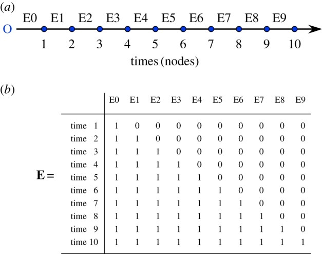
First step of AEM analysis: for a regular time series (a), construction of the nodes-by-edges matrix E (b). Letter ‘O’ represents the point of origin of the process before the actual data points. In this example, the nodes represent times 1–10; the edges (columns of E) are labelled E0–E9; they all have the same weight in this example. (Online version in colour.)

In spatial modelling, MEM eigenfunctions were not originally designed to model the directional component of complex spatial models. That role was devoted to the AEM method, which was designed to adequately model gradients generated by directional processes in complex spatial situations. That is different for time series, which are physically one-dimensional and where the action of a directional process can only manifest itself by the production of a single gradient along the series. In time-series analysis, MEM and AEM modelling can both be used for analysing the undetrended data and estimate the directional component of variation, as shown in the electronic supplementary material, appendix S1. Figure 2 compares dbMEM and AEM eigenfunctions for a time series with 50 equispaced points. The AEM eigenfunctions selected during analysis of the Case study data are shown in the electronic supplementary material, figure S3.6.

6. Local contributions to beta diversity

LCBD are comparative indicators of the ecological uniqueness of the sampling units [2]. For community composition data transformed in an appropriate way (Hellinger or chord transformation, see [2]), LCBD indices are the row sums of the data in matrix Y transformed by centring each column and squaring. For dissimilarity matrices, LCBD indices are the diagonal values in the Gower-centred dissimilarity matrix [2]. In ordination diagrams, an LCBD index is the squared distance of a site to the multivariate centroid of the plot. Sites located far from the centroid have unusual species compositions.

LCBD indices indicate how much each observation contributes to beta diversity; a site with average species composition would have an LCBD value of 0. Large LCBD values may indicate sampling units that have high conservation value or, perhaps, degraded and species-poor sites that are in need of restoration. They may also correspond to special ecological conditions, or result from the disturbance effect of invasive species on communities. LCBD indices take zero or positive values, and they sum to 1 if they are divided by the total sum of squares of the data matrix Y or the trace of the Gower-centered dissimilarity matrix. LCBD values can be mapped, allowing for visual assessment of their geographical, temporal or space–time variation. As an example, a geographical map of LCBD indices of the spring surveys at 27 sites, summed over the sampling years, is shown in the electronic supplementary material, figure S3.10. Temporal and space–time maps of LCBD indices are shown in §8.

7. Further methods for community time-series analysis

To test hypotheses about changes in the environment induced by man, ecologists sample ecosystems repeatedly over time without replication at the level of the sampling units (sites); in this way, the sampling effort can maximize the size of the area covered by the study. Classical statistical methods do not allow one to test the interaction between space and time for lack of replicate observations. Assessing that interaction is, however, of great interest to ecologists, because a significant interaction would indicate that the spatial structure of the response data has changed through time (and conversely), revealing for example the signature of climate change on ecosystems. Legendre et al. [14] described a method to solve that problem. In a nutshell, the method consists of representing space and time by spatial and temporal eigenfunctions (e.g. MEM or AEM eigenfunctions) in two-way ANOVA. This methodological development is important for the analysis of long-term monitoring data, including systems under anthropogenic inflfluence. To carry out the calculations, package STI in R is available on the web page https://sites.google.com/site/miqueldecaceres/software.

Multiscale ordination (MSO; [15,16]) combines multivariate variograms with simple or canonical ordination to determine whether or not explanatory variables are responsible for the spatial correlation observed in response data Y, for example community composition, and at which distance classes their effect is important. With simple ordination such as PCA, MSO partitions the variance of the ordination axes among distance classes to identify the axes that display spatial structure and determine whether it differs among axes. With canonical ordination methods, the analysis can incorporate matrices of environmental variables and eigenfunctions (MEM or AEM) to determine whether the spatial/temporal correlation in Y is due to induced spatial dependence or the presence of spatial/temporal autocorrelation in the response data. This method is available in R in function ‘mso’ of package ‘vegan’.

Consider the relationship between an explanatory (x) and a response variable (y) across space or time. For linear relationships, a significant correlation is interpreted as support for the hypothesis that x may affect y. Because y may react to different environmental factors at different scales, one may be interested in determining at which scale(s) x is an important predictor of y. Guénard et al. [17] developed multiscale codependence analysis (MCA) to address that question and test the significance of the correlations between two variables at different scales. The method is based on spatial eigenfunctions, MEM or AEM, which correspond to different and identifiable scales. It produces a vector of codependence coefficients corresponding to the different scales modelled by the eigenfunctions. Each codependence coefficient can be tested for significance. The R package codep is available to carry out MCA for bivariate data.

These three methods have been reviewed by Legendre & Legendre [1]. Additional methods based on spatial eigenfunctions were described by [4] for multiscale spatial analysis. They can readily be applied to multivariate time series.

8. Case study

Electronic supplementary material, appendix S2, contains a full practical session, using the R language, describing the analysis of an ecological survey of Chesapeake Bay, on the Atlantic coast of the USA, using the methods described in the paper. The publicly available Chesapeake Bay Benthic Monitoring Programme data used here were obtained from Versar Inc., Columbia, MD, USA (http://www.baybenthos.versar.com) who collected them for the Chesapeake Bay Programme (http://www.chesapeakebay.net/). The data are provided in an RData file. Here, we ask questions about these data and describe analyses that can be used to answer them.

From the Chesapeake Bay data, we included in our RData file the 27 fixed sampling sites (see the electronic supplementary material, figure S3.2) from the ‘Maryland Data Sets’ of the monitoring program (see http://www.baybenthos.versar.com/data.htm) and the 13 years for which spring and autumn sampling were present, for a total of 26 sampling events per site, from May 1996 to October 2008. There are 351 data rows corresponding to spring surveys and the same number for autumn surveys. Explanatory variables describe sediment (seven variables) and water quality (seven variables). A separate data table contains the latitude and longitude coordinates of the sites. The response data are the abundances of 205 benthic macrofaunal taxa (203 invertebrates and two chordates) captured at the sampling sites. Detailed descriptions of our data selection and the resulting tables are found in section 1.1 of the electronic supplementary material, appendix S2.

(a). Macrofauna time series, site 40 data

First, we look at site 40, located in the upper (brackish) course of the Potomac River, and model the macrofauna using dbMEM analysis. No significant linear temporal trend was present in the multivariate time series (r² = 0.0793, p = 0.053; electronic supplementary material, appendix S2, §3.2, Practicals), so the data will not be detrended prior to eigenfunction analysis. The dbMEM and AEM methods are equally suitable to analyse multivariate data for temporal structure.

(i). Moran's eigenvector map and asymmetric eigenvector map analyses of time series, site 40 data

The model containing the 12 MEMs that model positive temporal correlation was globally significant: r² = 0.5885, p < 0.05. The first two axes were significant (p < 0.05). The model containing the 13 MEMs modelling negative temporal correlation was not globally significant (r² = 0.4115, p > 0.90), but it produced a significant canonical axis (p < 0.05), which is worth looking at: it illustrates the oscillation between the spring and autumn communities (see the electronic supplementary material, figure S3.3).

Eight MEMs were selected (p-values < 0.05), six modelling positive temporal correlation (2, 3, 5, 6, 8 and 11) and two modelling negative correlation (21 and 25). These eigenfunctions are plotted along time in the Practicals, §3.2.1 (see the electronic supplementary material, figure S3.4). Examine the RDA models or the positively and negatively correlated MEMs plotted along the years (Practicals, §3.2.1, electronic supplementary material, figure S3.5) where the following can be seen.

• — Two significant RDA axes represent the positive correlation model, models 1 and 2, which are orthogonal to each other (i.e. linearly independent) and thus contain complementary information. They display large fluctuations across 13 years. These models were interpreted by stepwise selection in multiple regression. For MEM model 1, the North Atlantic Oscillation (NAO, added to the database for this analysis) and total nitrogen explained r²_adj = 0.2570 of the variation. For MEM model 2, no explanatory variable was selected and significant.

• — The single significant RDA axis representing the negative correlation model is interesting because it shows an important, significant alternation in community structure between the spring (the positive model values in the electronic supplementary material, figure S3.5) and autumn samplings (the negative values). (Note that the signs along eigenfunction models may be inverted when the calculations are done on different computers or using different software.) In stepwise selection against the available environmental variables, that axis is well explained by the season factor (r² = 0.8583).

The canonical axes obtained using AEM eigenfunctions (see the electronic supplementary material, figure S3.7) were similar to the MEM models (Practicals, §3.2.2 and electronic supplementary material, figure S3.5). RV coefficients between the groups of MEM and AEM eigenfunctions were 0.9129 for the 12 functions modelling positive temporal correlation and 0.9196 for the 13 functions modelling negative correlation, indicating that the MEM and AEM sets of eigenfunctions should have similar explanatory powers. The RV coefficient is a multivariate generalization of the Pearson correlation to compare two datasets [18,19].

A scalogram of the relative importance of the 12 dbMEM eigenfunctions modelling positive temporal correlation is shown in the electronic supplementary material, figure A3.8 (Practicals, §3.2.3). The contributions of the eigenfunctions to modelling the variation of the macrofauna series are given by the semipartial r² of each MEM analysed in the presence of all other MEMs, but the significance is the one found during forward selection of the eigenfunctions, as in [1]. Scalograms are especially useful when there are many significant MEMs (not the case here) and one wants to group them into submodels corresponding to broad, middle and fine scales.

(ii). Variation partitioning involving environmental variables and distance-based Moran's eigenvector maps

Partitioning the variation of the macrofauna time series at site 40 with respect to environmental and MEM explanatory variables is illustrated in figure 5 (Practicals, §3.3). Among the available environmental variables, only salinity was retained by forward selection. Its influence is represented by the upper-left circle. The upper-right circle represents the variation explained by the six MEMs modelling positive temporal correlation; this is the dominant explanatory factor in this partitioning. The lower circle represents the variation explained by the two MEMs modelling negative correlation. The partial contribution of salinity in the presence of the two MEM models is not significant, but the partial contributions of the two MEM models are significant, showing that they represent interesting fractions of variation that remains unexplained by the available environmental variables.

Figure 5.

Venn diagram illustrating the result of variation partitioning of the macrofauna time series at site 40 with respect to environmental (salinity, upper-left circle) and MEM explanatory variables (upper-right circle: six selected MEM eigenfunctions with positive Moran I; lower circle: two selected MEM eigenfunctions with negative Moran I). The fractions of variation displayed in the diagram are computed from adjusted r². Circles are not drawn to scale.

(iii). Multivariate correlogram, multivariate regression tree

A multivariate correlogram was computed for the same site 40 data (Practicals, §3.4; electronic supplementary material, figure S3.9). The correlogram shows that observations 1 year apart (second distance class along the abscissa) were highly positively correlated. The correlation between adjacent observations (first distance class), which are from different seasons, was marginally significant (p = 0.048, although p-values may depend on the permutation run) and weaker. The other distance classes showed no significant temporal correlation.

A multivariate regression tree (MRT) was used as a time-constrained clustering method to identify one or several breakpoints in the data series (Practicals, §3.5). The analysis identified one breakpoint separating observations 1–6 (years 1996–1998, spring and autumn) from years 1999 to 2008. This is consistent with the small variation among the first six observations along the MEM model of positive axis 1 in the electronic supplementary material, figures S3.3 and S3.5. Other examples of time-constrained clustering by MRT are provided in [9,20].

Space–time analysis of LCBD indices based upon the Hellinger distance (Practicals, §5), allowed for the unambiguous identification of unique sites and site–year combinations (see the electronic supplementary material, figures S3.12 and S3.13). It also revealed that the year effect was negligible during the autumn, and that the site effect was the most important in explaining LCBD scores, regardless of season. The NAO and water quality variables (notably salinity and conductivity) explained a smaller fraction of variation. Section (c) of the Case study, which describes the contributions of the spatio-temporal sampling units to beta diversity, is presented in the electronic supplementary material, appendix S4.

(b). Analysis of subsets of the sites

(i). Two-way temporal MANOVA of a subset of five sites

Sites 22, 23, 201, 202 and 203 located around the large inlet near the city of Baltimore were selected. Site 203 somewhat stood apart from the others in terms of water quality, but not in temperature, and these sites exhibited gradients along sampling years in terms of sedimentary variables, notably moisture, total carbon and total nitrogen content.

We will examine the response of the macrofauna to factors year and season using a two-way MANOVA (i.e. multivariate ANOVA) with permutation tests computed by RDA (Practicals, §4.1). The design is balanced with 5 observations in each cell of the year-by-season contingency table. The two factors are represented by Helmert contrasts. The interaction is generated by computing the products of all the Helmert variables coding for the two factors, as described in the Practicals.

The hypothesis that the within-group covariance matrices were homogeneous was not rejected by a test of multivariate homogeneity. We could thus proceed with the analysis of variance. The interaction was not significant and we could move to the analysis of the main factors. The tests found the variation explained by the two main factors to be significant (p < 0.05). However, factor season (r² = 0.1538) explained more of the macrofauna variation than factor year (r² = 0.1000).

(ii). Space-time variability among sites and years

Now we selected two groups of three sites, located in different regions of Chesapeake Bay. Sites 43, 44 and 47 were in the Potomac River estuary in the southwest of the bay whereas sites 201, 202 and 203 were in the large inlet near Baltimore (electronic supplementary material, appendix S3, figure S3.2). The six sites formed two groups with three replicates each. The sites within each group were far enough from one another that the faunal data should not be pseudoreplicated. We tested whether the site and year factors could explain the multivariate dispersion between these two groups of geographically distant sites during each season (Practicals, §4.2).

Comparing the spring survey data, we failed to reject the hypothesis of homogeneity of the multivariate within-group covariance matrices, and we found that the interaction between factors site and year was not significant (p ≈ 0.50). Similar results were found for the fall survey data.

Testing the effect of the main factors for the spring data, we found highly significant variation between the groups of sites (p < 0.01, r² = 0.1530) and among the years (p < 0.01, r² = 0.2303). For the fall data, we found highly significant variation between the groups of sites (p < 0.01, r² = 0.2104) but not among the years (p ≈ 0.80, r² = 0.1137). Hence the macrofaunal differences between the two groups of sites were clear during both seasons. However, the differences among years were stronger and more consistent in the spring than in the fall, suggesting that the outcome at the end of the growing season (fall) was rather stable from year to year despite marked variations at the spring starting points.

Sections 8b(i,ii) reported results of two-way MANOVAs with replication, which posed no particular problem for the test of the interaction between factors. When there is no replication, it is still possible to test the interaction between space and time using the method proposed by [13], which is based upon MEM coding of the factors instead of Helmert contrasts. A package of R functions is available, as a supplement to that paper, to carry out the calculations.

9. Conclusion

Ecologists study communities of living beings because they represent the best response data available to answer questions about species–environment relationships and test theories about productivity, stability, and the generation and maintenance of biodiversity in ecosystems. Ecological studies are designed to analyse the variance of the observed response data; most investigations aim at studying spatial, temporal, or experimentally controlled variation.

In the spatial context, Whittaker [21] described the spatial organization of biodiversity and called beta diversity the variation in community composition among sites in a geographical region of interest. Beta diversity can be analysed as either a directional change along spatial, temporal or environmental gradients, or a non-directional change in composition among sampling units without reference to any explicit gradient [22–24]. The total variance (Var_total) of a community composition data table is an appropriate estimate of beta diversity in the latter context [1,2,23,24].

In studies through time aimed at elucidating temporal processes, that concept can readily be extended to the variation in the community composition among temporal sampling units, where it can be referred to as temporal beta diversity. A further step is to apply the concept to spatio-temporal data such as the Chesapeake Bay macrofaunal data analysed in §8.

This total variance can be computed either from the raw species presence–absence or abundance data table, properly transformed or through one of several dissimilarity coefficients developed and used by ecologists for the analysis of community composition data [2]. This last step links the concept of beta diversity to all methods of analysis developed and used by ecologists to decompose the total variance or the total sum of squares (SS_Total) of the community composition data table, namely partitioning SS_Total among ordination or canonical ordination axes by PCA or RDA; partitioning SS_Total with respect to one or several factors structuring the data table by ANOVA; partitioning total beta into LCBD indices, either among sites, times or spatio-temporal observations, as shown in this paper; SS_Total can be partitioned with respect to two or more matrices of explanatory variables by variation partitioning; last but not least, SS_Total can be partitioned among spatial or temporal observation scales by spatial eigenfunction analysis (MEM, AEM), scalogram, multivariate correlogram or MSO analysis.

This review describes, for the first time to our knowledge, the statistical theory of eigenfunction-based methods for multivariate time-series analysis. Electronic supplementary material, appendix S2, contains a detailed description of how to carry out the calculations using the R statistical language, and how to use the software. The case study illustrates the interest of the eigenfunction-based methods, which allow ecologists to describe the multiscale temporal structure of community composition data observed at a site through the methods mentioned in the previous paragraph. Other recently developed methods are shown in §8 to be applicable to community composition time series: multivariate correlograms, MRT analysis as a form of constrained clustering, one-way and two-way MANOVA and the analysis of local (temporal) contributions to beta diversity.

Data accessibility

The Chesapeake case study data are available in the electronic supplementary material, appendix S5.

Funding statement

This research was supported by a Natural Sciences and Engineering Research Council of Canada (NSERC) research grant to P.L. and a Centre National de la Recherche Scientifique (CNRS) research grant to O.G.

References

- 1.Legendre P, Legendre L. 2012. Numerical ecology, 3rd English edition. Amsterdam, The Netherlands: Elsevier Science BV [Google Scholar]
- 2.Legendre P, De Cáceres M. 2013. Beta diversity as the variance of community data: dissimilarity coefficients and partitioning. Ecol. Lett. 16, 951–963 (doi:10.1111/ele.12141) [DOI] [PubMed] [Google Scholar]
- 3.Hutchinson GE. 1957. Concluding remarks. Cold Spring Harb. Symp. Quant. Biol. 22, 415–427 (doi:10.1101/SQB.1957.022.01.039) [Google Scholar]
- 4.Dray S, et al. 2012. Community ecology in the age of multivariate multiscale spatial analysis. Ecol. Monogr. 82, 257–275 (doi:10.1890/11-1183.1) [Google Scholar]
- 5.Hu X-S, He F, Hubbell SP. 2006. Neutral theory in macroecology and population genetics. Oikos 113, 548–556 (doi:10.1111/j.2006.0030-1299.14837.x) [Google Scholar]
- 6.Borcard D, Legendre P. 2002. All-scale spatial analysis of ecological data by means of principal coordinates of neighbour matrices. Ecol. Model. 153, 51–68 (doi:10.1016/S0304-3800(01)00501-4) [Google Scholar]
- 7.Blanchet FG, Legendre P, Maranger R, Monti D, Pepin P. 2011. Modelling the effect of directional spatial ecological processes at different scales. Oecologia 166, 357–368 (doi:10.1007/s00442-010-1867-y) [DOI] [PubMed] [Google Scholar]
- 8.Borcard D, Legendre P, Avois-Jacquet C, Tuomisto H. 2004. Dissecting the spatial structure of ecological data at multiple scales. Ecology 85, 1826–1832 (doi:10.1890/03-3111) [Google Scholar]
- 9.Borcard D, Gillet F, Legendre P. 2011. Numerical ecology with R. Use R! series. New York, NY: Springer Science [Google Scholar]
- 10.Dray S, Legendre P, Peres-Neto PR. 2006. Spatial modelling: a comprehensive framework for principal coordinate analysis of neighbour matrices (PCNM). Ecol. Model. 196, 483–493 (doi:10.1016/j.ecolmodel.2006.02.015) [Google Scholar]
- 11.Griffith DA. 2000. A linear solution to the spatial autocorrelation problem. J. Geogr. Syst. 2, 141–156 (doi:10.1007/PL00011451) [Google Scholar]
- 12.Guénard G, Legendre P, Peres-Neto PR. 2013. Phylogenetic eigenvector maps: a framework to model and predict species traits. Methods Ecol. Evol. 4, 1120–1131 (doi:10.1111/2041-210X.12111) [Google Scholar]
- 13.Blanchet FG, Legendre P, Borcard D. 2008. Modelling directional spatial processes in ecological data. Ecol. Model. 215, 325–336 (doi:10.1016/j.ecolmodel.2008.04.001) [Google Scholar]
- 14.Legendre P, De Cáceres M, Borcard D. 2010. Community surveys through space and time: testing the space-time interaction in the absence of replication. Ecology 91, 262–272 (doi:10.1890/09-0199.1) [DOI] [PubMed] [Google Scholar]
- 15.Wagner HH. 2003. Spatial covariance in plant communities: integrating ordination, variogram modeling, and variance testing. Ecology 84, 1045–1057 (doi:10.1890/0012-9658(2003)084[1045:SCIPCI]2.0.CO;2) [Google Scholar]
- 16.Wagner HH. 2004. Direct multi-scale ordination with canonical correspondence analysis. Ecology 85, 342–351 (doi:10.1890/02-0738) [Google Scholar]
- 17.Guénard G, Legendre P, Boisclair D, Bilodeau M. 2010. Multiscale codependence analysis: an integrated approach to analyze relationships across scales. Ecology 91, 2952–2964 (doi:10.1890/09-0460.1) [DOI] [PubMed] [Google Scholar]
- 18.Escoufier Y. 1973. Le traitement des variables vectorielles. Biometrics 29, 751–760 (doi:10.2307/2529140) [Google Scholar]
- 19.Robert P, Escoufier Y. 1976. A unifying tool for linear multivariate statistical methods: the RV-coefficient. Appl. Stat. J. R. St. C 25, 257–265 (doi:10.2307/2347233) [Google Scholar]
- 20.Mines C, Ghadouani A, Yan ND, Legendre P, Ivey GN. 2013. Examining shifts in zooplankton community variability following biological invasion. Limnol. Oceanogr. 58, 399–408 (doi:10.4319/lo.2013.58.1.0399) [Google Scholar]
- 21.Whittaker RH. 1972. Evolution and measurement of species diversity. Taxon 21, 213–251 (doi:10.2307/1218190) [Google Scholar]
- 22.Vellend M. 2001. Do commonly used indices of beta-diversity measure species turnover? J. Veg. Sci. 12, 545–552 (doi:10.2307/3237006) [Google Scholar]
- 23.Legendre P, Borcard D, Peres-Neto PR. 2005. Analyzing beta diversity: partitioning the spatial variation of community composition data. Ecol. Monogr. 75, 435–450 (doi:10.1890/05-0549) [Google Scholar]
- 24.Anderson MJ, et al. 2011. Navigating the multiple meanings of β diversity: a roadmap for the practicing ecologist. Ecol. Lett. 14, 19–28 (doi:10.1111/j.1461-0248.2010.01552.x) [DOI] [PubMed] [Google Scholar]
Associated Data
This section collects any data citations, data availability statements, or supplementary materials included in this article.
Data Availability Statement