Spatial scale and sampling resolution affect measures of gap disturbance in a lowland tropical forest: implications for understanding forest regeneration and carbon storage

Abstract

Treefall gaps play an important role in tropical forest dynamics and in determining above-ground biomass (AGB). However, our understanding of gap disturbance regimes is largely based either on surveys of forest plots that are small relative to spatial variation in gap disturbance, or on satellite imagery, which cannot accurately detect small gaps. We used high-resolution light detection and ranging data from a 1500 ha forest in Panama to: (i) determine how gap disturbance parameters are influenced by study area size, and the criteria used to define gaps; and (ii) to evaluate how accurately previous ground-based canopy height sampling can determine the size and location of gaps. We found that plot-scale disturbance parameters frequently differed significantly from those measured at the landscape-level, and that canopy height thresholds used to define gaps strongly influenced the gap-size distribution, an important metric influencing AGB. Furthermore, simulated ground surveys of canopy height frequently misrepresented the true location of gaps, which may affect conclusions about how relatively small canopy gaps affect successional processes and contribute to the maintenance of diversity. Across site comparisons need to consider how gap definition, scale and spatial resolution affect characterizations of gap disturbance, and its inferred importance for carbon storage and community composition.

1. Introduction

In mature tropical forests, the most common type of disturbance initiating forest regeneration is the creation of canopy gaps by tree falls [1]. Consequently, the extent, frequency and distribution of canopy gaps across space and time play a central role in our understanding of community dynamics as well as key ecosystem processes, notably carbon storage. Gap disturbance regimes are typically characterized by the proportion of forest area in gaps (the gap area fraction) and by the gap-size-frequency distribution (the relative frequency of gaps across gap-size classes). Common values for the gap area fraction of tropical forests range from less than 1 to 10% [2–7], but values more than 10% are also sometimes reported [8,9]. The gap-size-frequency distribution has often been found to follow a power-law distribution [10–12], but deviations from this pattern are also possible [13].

The relationship between the gap area fraction and carbon storage or community dynamics is likely to be relatively straightforward; an increase in the gap area fraction implies reduced basal area and therefore above-ground biomass (AGB), and potentially increased representation in the forest stand of light-demanding species with low wood density that recruit exclusively in newly formed gaps [14]. On the other hand, the influence of variation in the gap-size distribution on community and ecosystem processes is less clear. If species recruitment success is influenced not only by the presence of gaps, but also by gap size, then changes in the gap-size-frequency distribution could result in compositional shifts in tree communities with impacts on AGB.

The gap-size distribution is also critical in scaling estimates of AGB from the plot to the landscape scale. Large canopy gaps (1000–10 000 m²), resulting from infrequent windstorms or landslides, influence AGB at the landscape scale [15] but may be inadequately sampled in forest plot datasets, even when the plot size is quite large. Based on simulations [11], the minimum area required to generate unbiased estimates of fluxes in AGB was found to depend largely on the relative frequency of large canopy gap disturbances.

To date, most estimates of gap disturbance are based on interpolations from ground surveys of canopy height made at a grid of sample points [16–18]. As these studies are limited in spatial extent (1–50 ha), they are unlikely to adequately characterize rare, large-scale disturbance events [11]. In the most detailed analysis of gap disturbance rates based on ground data, Hubbell et al. [16] recorded the frequency of forest gaps in a 50 ha plot on Barro Colorado Island (BCI), Panama. Gaps were defined as sample points on a 5 m grid with less than 5 m canopy height, with adjacent low canopy points (excluding diagonals) aggregated into individual gaps. Analysis of 1284 gaps identified this way in 1983, 1988 and 1999 revealed that the BCI plot is dominated by small gaps, with more than 99% of gaps less than 400 m², and the largest gap 1150 m² [16].

By contrast, remotely sensed data on gap disturbance based on satellite imagery often fails to detect the small gaps that characterize the BCI plot. In a recent study, Chambers et al. [19] used Landsat imagery to characterize the gap-size distribution of the central Amazon. Their imagery could only resolve gaps resulting from clusters of more than eight treefalls (approx. 900 m²). When these data were combined with existing plot data, they inferred that infrequent large gaps account for 9–17% of tree mortality on the landscape. They further argued that these are the most important gaps influencing forest community composition and carbon storage, and that consideration of relatively large, rare disturbances is critical to evaluating hypotheses for how disturbance influences community assembly [19].

The mismatch in size between gaps that can be detected from satellite imagery, and those that mostly occur in plots, precludes a more detailed examination of how gap size influences species composition, and therefore exerts indirect effects on AGB. The conclusion that gaps more than 900 m² play a disproportionate role in determining community composition [19] was based on the assumption that smaller gaps do not initiate secondary succession (i.e. the replacement of slow-growing shade-tolerant tree species with short-lived fast-growing pioneers). In turn, this assumption was based on the Hubbell et al. [16] analysis of species composition in gaps in the BCI plot. Hubbell et al. [16] found that gap size had no influence on species richness when expressed on a per-stem basis, and therefore did not support the predictions of the intermediate disturbance hypothesis [20].

Here, we use Light Detection and Ranging (from here on LiDAR) to obtain canopy height estimates across a 1500 ha tropical forest landscape at BCI. Metre-scale spatial resolution in these measurements allows quantification of the gap frequency distribution from the smallest scale detectable from ground surveys to the largest gaps observed on satellite imagery. Furthermore, high (centimetre-scale) accuracy in the measurement of canopy height achievable using LiDAR allows us to examine in detail how the use of canopy height thresholds to define gaps influences gap disturbance metrics. This is an important area for initial exploration as different disturbance processes (landslides, fallen trees and snapped trees) may differ in the initial canopy height profile that they generate, and may differ in probability that the gaps they form undergo secondary succession.

Our specific objectives using LiDAR data were therefore: (i) to determine how estimates of the gap area fraction and size distribution are influence by the spatial extent of the study area, and the criteria used to define gaps; (ii) to assess whether previous estimates of gap area fraction and the gap-size distribution measured at the plot scale adequately capture the characteristics of gap disturbance observable at the landscape scale on BCI; and (iii) to explore how well ground-based sampling of canopy heights implemented in previous studies [16] can estimate the size and location of forest gaps. If ground-based surveys are poor predictors of the size and location of gaps, then previous analysis of how gap size influences species composition may need to be re-evaluated, with implications for theories of how species diversity is maintained, and for how even relatively small gaps impact AGB.

2. Material and methods

(a). Study site

This study was conducted at BCI, Panama (9°9′ N, 79°51′ W) (figure 1). BCI is a 1500 ha island supporting semi-deciduous lowland moist forest. Average annual rainfall is 2600 mm, with a pronounced dry season between December and April [21]. The western half of the island supports old growth forest 300–400 years old. The eastern half of the island is a mosaic of secondary forests 80–150 years old, resulting from clearing during the late 1800s for small farm settlements [22]. All human disturbances other than those related to scientific research stopped in 1923, when BCI was declared a reserve [23]. A 50 ha forest-monitoring plot located in the centre of BCI is composed of mostly of old growth forest with 2 ha of secondary forest about 100 years old [24]. The majority of the plot is on a plateau at an elevation of 120–160 m above sea level, with gentle slopes to the south and east. Mean canopy height is 24.6 ± 8.2 m s.d. and AGB is estimated 281 ± 20 Mg ha⁻¹ [24].

Figure 1.

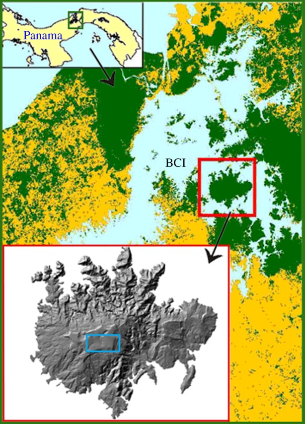
Location of BCI in the Panama Canal Area, Panama. The 50 ha forest-monitoring plot is shown as a rectangle located in the centre of the island. (Online version in colour.)

(b). Canopy height data

LiDAR data were acquired during August and September 2009 with a multi-pulse scanning laser altimeter (Optech ALTM Gemini system; BLOM Sistemas Geoespaciales SLU, Madrid, Spain). The number of returns at the landscape ranged between 4 and 27 points per square metre; point density at the 50 ha plot ranged between 9 and 27 points per square metre. Point clouds were used to generate a digital terrain model and digital surface model with 1 m² pixels; additional models with 0.25 m² pixels were generated for the 50 ha plot. Heights were calculated by subtracting elevations from these models. Estimated vertical errors were smaller than 15 cm (BLOM 2009, unpublished data). The geo-positioning of the 50 ha plot was based on the known location of coordinates of the corners (with less than 1 m positional error) [25].

(c). Effects of gap height and plot size on the gap-size distribution

Gaps were defined as contiguous areas with a canopy height lower than a threshold maximum canopy height detected with LiDAR. The minimum gap size included in this study was 5 m², as we assume that smaller gaps are unlikely to influence tree recruitment or carbon storage. Gap area was resolved to the nearest square metre. Three different threshold top-of-canopy heights commonly used in other studies, 2, 5 and 10 m, were used to assess the implications of differences in gap definition for the gap-size distribution and gap area fraction. Gap maps were derived for the entire landscape based on these definitions. To evaluate whether plot size has an effect on the fraction of gap area and the gap-size distribution, we used plot sizes of 10, 50 and 100 ha. For every combination of plot size and gap height, 1000 plots were randomly generated throughout a 992 ha polygon, which corresponded to the portion of the landscape that was able to fit plots of all sizes. For every plot, the fraction of gap area and the observed distribution of gaps were recorded; these were also recorded for the 992 ha polygon and the entire landscape, which has an area of 1484 ha, excluding the shores and the laboratory clearing. The gap-size distribution for every plot was then fit to a power-law probability distribution. In a discrete power-law with parameter λ, the probability for gap size k is given by

2.1

Lambda (λ) is related to the ratio of small gaps to large gaps; larger values of λ indicate a smaller relative frequency of large gaps. Maximum-likelihood estimates (MLEs) for λ were calculated by minimizing the negative log-likelihood function. We calculated standard errors for λ, based on the marginal likelihood (I, equation (2.2)), so that

2.2

The 95% CIs were calculated for each estimate of λ, based on the standard error (equation (2.2)) and a t-distribution [26]. Mann–Whitney tests were used for the contrasts of means and Levene tests were used for the contrasts of variances for the distributions of λ across plot sizes.

To better understand the effects of the threshold canopy height used to assign gaps on the gap-size distribution, gap maps were generated for the entire landscape for all maximum gap heights between 1 and 15 m. Gap-size-frequency distributions were fit to a power-law and fraction of gap area was calculated for the landscape.

(d). Height contrast: field versus light detection and ranging

To assess the importance of gap aggregation errors that might result from field surveys of canopy height, we developed a new canopy height model for the 50 ha plot (figure 2). Our approach simulated the field data collected by Hubbell et al. [16], where a single canopy height measurement was taken on a 5 m grid and used to represent the canopy height of a 25 m² quadrat of forest and a maximum height of 5 m was used to define gaps. Accordingly, we subsampled the LiDAR data at the same scale and assigned canopy heights from 1 m² plots to the surrounding 25 m². Aggregation errors are defined here as the errors in canopy height estimates resulting from a reduced sampling frequency. Two types of aggregation error can occur in the estimation of gap spatial distribution and extent: (i) commission error, where high canopy forest is wrongly classified as a gap using low-resolution canopy height data, and (ii) omission error, where gap is wrongly classified as high canopy forest.

Figure 2.

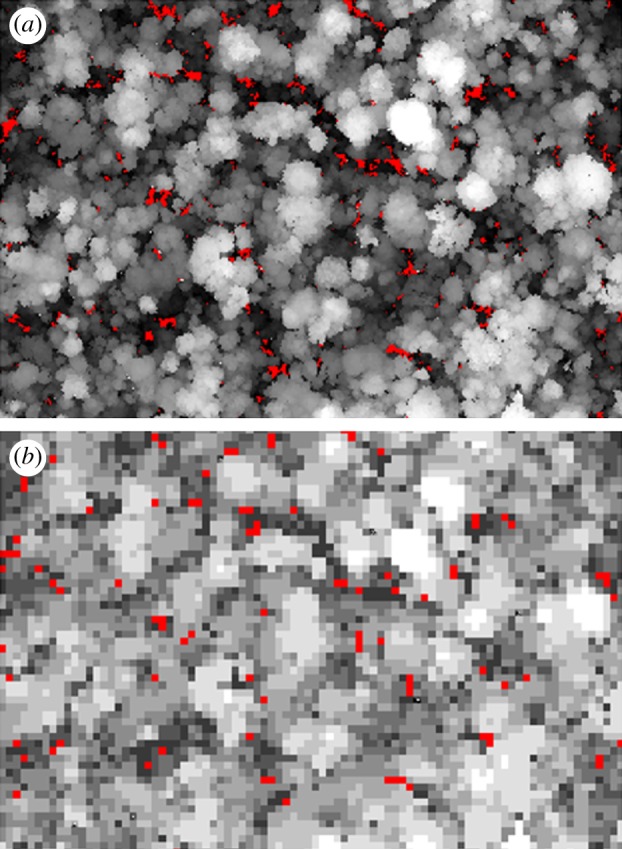
A 10 ha sample of the BCI 50 ha plot selected to show canopy height (greyscale) and gaps less than 5 m canopy height (red). (a) Fine spatial resolution typical of LiDAR (1 m² pixels) and (b) coarse spatial resolution typical of field data (25 m² pixels).

For both high-resolution (the full LiDAR) and low-resolution (simulated field data) canopy height models, we then generated gap-size-frequency distributions and fit power-law functions. Parameter estimates were calculated using MLE for the gap-size distribution generated using 1 m² quadrats. For the gap-size distribution generated with 25 m² quadrats, MLE could not be used owing to the small number of resulting gap-size classes; a logarithmic transformation followed by ordinary least squares (OLSs) was used instead. To make both gap-size distributions comparable, we also applied a logarithmic transformation followed by an OLS fit to the gap-size distribution generated using 1 m² quadrats.

3. Results

(a). Gap fraction and gap-size distribution in the Barro Colorado Island forest

(i). Gap-size distribution

The mean power-law exponent (λ) of the gap-size distribution calculated from 1000 plots randomly generated throughout the landscape differed significantly among plot sizes (p < 0.005), but the differences were rather small (table 1). Standard error values for the 10 ha plots were two times greater than those for the 50 ha plots and three to four times greater than those for the 100 ha plots. The importance of large among-plot variation in λ at the small plot scale can be illustrated by comparing how frequently the λ of an individual plot falls outside the 99% CIs of λ calculated from repeatedly sampling throughout the landscape at the 100 ha scale (table 2). For example, the λ values of 44% of 10 ha plots classified using a 2 m maximum canopy height threshold would fall outside the 99% CIs for 100 ha plots.

Table 1.

Effect of plot size (ha), and the maximum canopy height cut-off used to define gaps (gap height) on the gap-size distribution (λ) and gap area (% of plot area in gaps). (Means are based on 1000 samples. The polygon comprises the 992 ha of the landscape where all plot sizes could fit. The landscape comprises the entire island, excluding the shores and the laboratory clearing, with an area of 1484 ha.)

	maximum canopy height cut-off for gap identification
	2 m		5 m		10 m
plot size	λ	gap area	λ	gap area	λ	gap area
10 ha	2.45 (0.42)	0.40 (0.20)	2.05 (0.25)	1.43 (0.70)	1.82 (0.11)	5.49 (2.18)
50 ha	2.36 (0.19)	0.42 (0.13)	2.00 (0.11)	1.52 (0.48)	1.77 (0.06)	6.08 (1.52)
100 ha	2.36 (0.13)	0.43 (0.09)	1.99 (0.05)	1.60 (0.34)	1.76 (0.04)	6.17 (1.12)
polygon	2.41 (0.03)	0.43 (n.a.)	2.03 (0.02)	1.59 (n.a.)	1.78 (0.01)	6.10 (n.a.)
landscape	2.37 (0.03)	0.41 (n.a.)	2.04 (0.01)	1.42 (n.a.)	1.78 (0.01)	6.04 (n.a.)

Table 2.

Effect of plot size (ha), and the maximum canopy height cut-off used to define gaps (gap height) on the probability of detecting an extreme value of λ. (The λ landscape is the mean value of λ at the landscape scale, and λ interval is the upper and lower 99% CIs of λ. Extreme values are defined as those outside the 99% CI (λ interval) calculated from the 100 ha plot sizes. The proportion of replicate plots of 10, 50, 100 ha with extreme values of λ are shown in the last three columns.)

			plot size (ha)
gap height (m)	λ landscape	λ interval	10	50	100
2	2.37	(2.10, 2.69)	0.44	0.12	0.01
5	2.04	(1.89, 2.16)	0.58	0.20	0.01
10	1.78	(1.68, 1.84)	0.46	0.13	0.01

The mean and standard error of the distribution of λ values decreased significantly (p < 0.005) with maximum canopy height threshold at the plot scale (table 1), and λ declined linearly with maximum canopy height at the landscape scale (figure 3a). When the maximum canopy height criterion used to identify gaps was relaxed from 2 to 10 m, λ decreased by 25%. This indicates that using criteria to include gap openings do not extend as close to the ground surface results in a higher relative abundance of large gaps.

Figure 3.

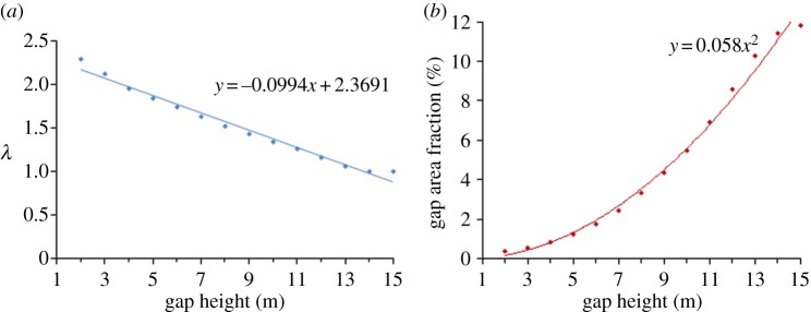
(a) Landscape pattern of λ and (b) fraction of gap area versus maximum gap height. All coefficients had p < 0.005; r² values for the regressions of λ and fraction of gap area versus maximum gap height were 0.981 and 0.996, respectively. (Online version in colour.)

(ii). Gap area fraction

The mean gap area fraction (per cent of the plot area in gaps) calculated from 1000 plots randomly generated throughout the landscape was relatively insensitive to the size of the sample plot (table 1). However, standard errors were significantly larger for the smallest plots (p < 0.005). As expected, gap area fraction was strongly influenced by the canopy height threshold used to delimit gaps. For a given plot size, both the mean and standard error of the distribution of gap area fraction values increased significantly (p < 0.005) with maximum canopy height. At the landscape scale, the gap area fraction increased as a second-order polynomial with maximum canopy height (figure 3b). Relaxing the canopy height threshold from 2 to 10 m resulted in more than a 20-fold increase in the gap area fraction.

(b). Comparison of light detection and ranging and field-based gap surveys

The effects of the spatial resolution of canopy height estimates on gap identification were assessed through comparison of LiDAR and simulated field data at the location of the 50 ha monitoring plot. The coarse spatial resolution of simulated field data, where a single 1 m² height measurement represents a 25 m² quadrat, led to substantial errors in canopy height estimation. Bias in the assessment of canopy height was particularly strong when the lowest canopy height class (0–5 m) was assigned to quadrats (figure 4), as, on average, simulated field data predicted canopy heights 8.2 m lower than those obtained using the full LiDAR data. The absolute value of bias progressively decreased as canopy height increased, with a mean value of 0.87 m for the more than 30 m height class.

Figure 4.

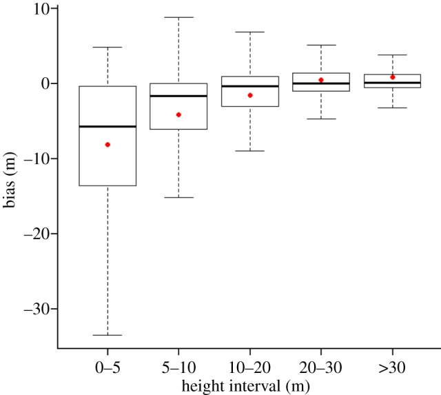
Box plot showing bias in canopy height estimates when using coarse spatial resolution for canopy height estimates across different canopy height intervals (from 0 to more than 30 m); bias is defined as the height of simulated field data with coarse spatial resolution minus the height from LiDAR data with fine resolution. Box plot shows the median, first and third quartile; the whiskers represent the maximum and minimum values of the distribution; dots show the mean bias for each height interval. (Online version in colour.)

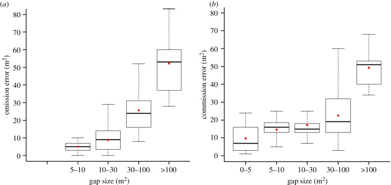
Simulated field data also led to errors in determining the frequency, location and extent of gaps (defined as areas with a canopy height less than or equal to 5 m [16]). An omission error of 50% (1 m² quadrats that are less than or equal to 5 m but are not classified as gaps) and a commission error of 79% (1 m² quadrats that are more than 5 m but are classified as gaps) were obtained (figures 5 and 6). Omission and commission errors both increased with gap size, but the accumulated error by gap size was similar across sizes because small gaps are much more abundant than large gaps.

Figure 5.

Box plots showing (a) omission and (b) commission errors by gap size when using coarse versus fine spatial resolution. Box plot shows the median, first and third quartile; the whiskers represent the maximum and minimum values of the distribution; dots show the mean value for each gap-size interval. The sum of omission errors is 50% and the sum of commission errors is 79%. (Online version in colour.)

Figure 6.

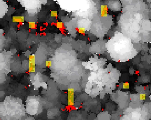
A 1.4 ha sample of the plot showing canopy height (greyscale). Red areas represent gaps defined using fine spatial resolution LiDAR, pale yellow areas indicate gaps defined using coarse spatial sampling that simulates field measurements, and orange areas show the areas classified as gaps under both schemes.

Gap-size-frequency distributions were generated for the simulated field data and the original LiDAR data and fitted to power-law functions. The gap-size distributions fitted using OLS were significantly different between the full LiDAR data and the simulated field data (figure 7). The gap-size distribution derived using the simulated field data had a significantly steeper decline in the number of gaps with increasing gap size (λ = 2.68) than that obtained using 1 m² quadrats (λ = 1.53; p < 0.005 for the estimates and the contrast test). However, it should also be noted that the value of λ is sensitive to the method used for fitting the gap-size distribution. For the 1 m² spatial resolution, where data were sufficient to use MLE, an estimate of λ of 2.05 (s.e. = 0.08) was obtained.

Figure 7.

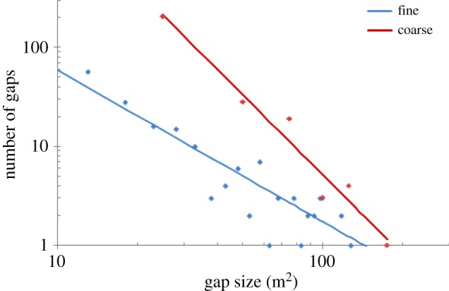
Gap-size-frequency distributions for the 50 ha plot generated using a fine spatial resolution (1 m² quadrats) and coarse resolution (25 m² quadrats). The distributions were fit to a power-law using OLSs after a logarithmic transformation (p < 0.005 for all parameter estimates). (Online version in colour.)

4. Discussion

(a). Effects of gap definition criteria and plot size on disturbance metrics

Canopy height-based definitions of gaps strongly influenced both the gap area fraction and the scaling parameter, λ, of the gap-size distribution. Increasing the minimum canopy height used to identify gaps from 2 to 10 m increased the gap area fraction from 0.4 to 6% and reduced λ from 2.4 to 1.8, indicating an increased relative abundance of large gaps. Clearly, gap definition criteria have important implications for the calculation of the gap area fraction and gap-size distribution. The dependency of λ on the canopy height threshold is particularly notable as this directly impacts inferences on whether forest dynamics plots fully capture landscape-level forest disturbance regimes [11]. However, it is unclear whether changes in disturbance metrics when the criterion for maximum canopy height is relaxed is entirely the consequence of capturing older gaps that are recovering canopy height, or if a higher canopy height threshold allows us to capture qualitatively different disturbances that may result in different community composition. Discerning these differences will require repeated use of high-resolution LiDAR, coupled with field studies to examine how canopy height impacts successional processes in gaps.

Our analyses showed that for the BCI forest, smaller plots do not produce systematically biased estimates of λ or the gap area fraction. However, variance for these parameters was much greater for smaller plots and dramatically so for plots of 10 ha size. Our results therefore provide an illustration of the ‘modifiable areal unit problem’ common in landscape ecology, where increased areal coverage results in a decline in variance of the measured parameter as landscape-level heterogeneity is smoothed [27,28]. On a practical level, we caution against interpreting rates of gap disturbance based on a few small plots. While large forest dynamics plots (50 ha) are likely to provide quite robust estimates of these parameters, a single estimate of λ may diverge greatly from the true landscape value.

(b). Efficacy of ground-based assessments of forest gaps

In addition to under-sampling landscape-level variation in gap disturbance, field-based identification of canopy gaps in forest plots may also be influenced by the spatial resolution of canopy height measurements (effectively the grain size). In our study, field data were simulated by applying the LiDAR-derived height measurement of a single 1 m² to every 25 m² grid cell across the BCI 50 ha forest dynamics plot following the methods of Hubbell et al. [16]. We found that using this method had a significant effect on the frequency distribution and spatial configuration of canopy heights. Overall, the canopy height distribution was only minimally affected by low-resolution sampling, because errors arising from the over- and under-estimation of canopy height mostly balanced out. However, the greatest errors in the estimation of height were observed for the lowest canopy height classes and led to substantial errors in the identification of gaps (figure 6).

The mismatch between the true spatial location of gaps, and those inferred by field sampling methods may have important implications for our assessment of how gaps affect biological processes, and in particular, the importance of light niches. Hubbell et al.'s [16] study of compositional and richness responses of the tree community to the inferred location of forest gaps on BCI led to an emphasis on dispersal limitation and ecological equivalency as dominant structuring processes in tropical forests. This conclusion may be premature. Seedling recruitment patterns and sapling growth rates vary in response to light availability at fine (less than 1 m) spatial scales, and consequently the link between demographic processes and gap disturbance will be obscured when large errors in their spatial location occur. Thus, the conclusion from Hubbell et al. [16] that, with the exception of pioneer species, the composition of the sapling community is largely decoupled from gap disturbance might well be influenced by a misidentification of the spatial location of gap areas.

(c). Implications for the estimation of above-ground biomass

The spatial scale dependency, canopy height threshold dependency and spatial resolution dependency of canopy height measurements all influence estimates of gap area fraction and λ, with implications for our understanding of how canopy disturbance events affect landscape-level AGB. Although our study cannot include the largest and rarest of disturbances that impact hundreds of hectares [15], such disturbances appear to be very rare [29,30]. Nonetheless, existing evidence that tropical forest biomass has been increasing in recent decades [20] is based on the assumption that networks of small forest plots adequately sample infrequent, large-scale forest disturbances that influence carbon storage on landscape scales [31].

Our results indicate that λ values of the smallest gap size for which we can generate a gap-size distribution (10 ha) falls outside the 99% CIs of the landscape-level λ approximately half the time, while those for 50 ha plots will fall outside 99% CIs less than 20% of times. Remote-sensed measures of gap disturbance may therefore need to be made at scales of 500–1000 ha, or greater, depending on landscape heterogeneity. By contrast, ground-based assessments of gap sizes may overestimate the magnitude of λ at any scale. We found that coarse sampling associated with field data produced a much steeper decline in the frequency of gaps with increasing gap size, than observed using the full LiDAR data, although the magnitude of λ was also influenced by the curve-fitting procedure (see also [29]).

Indirect impacts of λ on AGB via successional processes are more difficult to assess. Chambers et al. [19] argued that most gaps found in forest plots are too small, and do not provide sufficient light to result in compositional change in forests. While the study of Hubbell et al. [16] did not observe changes in species richness per stem across the range of gap sizes they measured in the BCI plot, they did observe a large increase in the frequency of pioneer species (from 7% in gaps less than 50 m² to 26% in gaps more than 400 m²). Likewise, Brokaw [2,29] measured how gap size influences regeneration patterns and found that pioneers readily colonized gaps less than 200 m², and that even the fastest growing species (Trema micrantha) could recruit in gaps less than 400 m². As these smaller gaps contribute to a much larger fraction of the landscape, assessment of how disturbance influences AGB requires inclusion of a wide range of gap sizes, including small gaps that cannot be easily detected from satellite imagery.

Data accessibility

The BCI LiDAR dataset is publically available from the Office of Bioinformatics, Smithsonian Tropical Research Institute. Enquiries can be made to J.W.D.

Funding statement

This study was financially supported by NSF grant no. 0939907, and with additional support from the Smithsonian Tropical Research Institute, University of Illinois, University of California Los Angeles and Clemson University.

References

- 1.Swaine MD, Whitmore TC. 1988. On the definition of ecological species groups in tropical rain forests . Vegetatio 75, 81–86 (doi:10.1007/BF00044629) [Google Scholar]
- 2.Brokaw NVL. 1985. Gap-phase regeneration in a tropical forest . Ecology 66, 682–687 (doi:10.2307/1940529) [Google Scholar]
- 3.Lawton R, Putz F. 1988. Natural disturbance and gap-phase regeneration in a wind-exposed tropical cloud forest . Ecology 69, 764–777 (doi:10.2307/1941025) [Google Scholar]
- 4.Jans L, Poorter L, Vanrompaey RSAR, Bongers F. 1993. Gaps and forest zones in tropical moist forest in Ivory-Coast . Biotropica 25, 258–269 (doi:10.2307/2388784) [Google Scholar]
- 5.Chandrashekara U, Ramakrishnan P. 1994. Vegetation and gap dynamics of a tropical wet evergreen forest in the Western Ghats of Kerala, India . J. Trop. Ecol. 10, 337–354 (doi:10.1017/S0266467400008014) [Google Scholar]
- 6.Marthews TR, Burslem DFRP, Phillips RT, Mullins CE. 2008. Modelling direct radiation and canopy gap regimes in tropical forests . Biotropica 40, 676–685 (doi:10.1111/j.1744-7429.2008.00431.x) [Google Scholar]
- 7.Kellner JR, Clark DB, Hubbell SP. 2009. Pervasive canopy dynamics produce short-term stability in a tropical rain forest landscape. Ecol. Lett. 12, 155–164 (doi:10.1111/j.1461-0248.2008.01274.x) [DOI] [PubMed] [Google Scholar]
- 8.Kapos V, Pallant E, Bien A, Freskos S. 1990. Gap frequencies in lowland rain-forest sites on contrasting soils in Amazonian Ecuador . Biotropica 22, 218–225 (doi:10.2307/2388531) [Google Scholar]
- 9.Ferreira de Lima RA, Zanforlin Martini AM, Gandolfi S, Rodrigues RR. 2008. Repeated disturbances and canopy disturbance regime in a tropical semi-deciduous forest . J. Trop. Ecol. 24, 85–93 [Google Scholar]
- 10.Satake A, Iwasa Y, Hakoyama H, Hubbell SP. 2004. Estimating local interaction from spatiotemporal forest data, and Monte Carlo bias correction . J. Theor. Biol. 226, 225–235 (doi:10.1016/j.jtbi.2003.09.003) [DOI] [PubMed] [Google Scholar]
- 11.Fisher JI, Hurtt GC, Thomas RQ, Chambers JQ. 2008. Clustered disturbances lead to bias in large-scale estimates based on forest sample plots . Ecol. Lett. 11, 554–563 (doi:10.1111/j.1461-0248.2008.01169.x) [DOI] [PubMed] [Google Scholar]
- 12.Kellner JR, Asner GP. 2009. Convergent structural responses of tropical forests to diverse disturbance regimes . Ecol. Lett. 12, 887–897 (doi:10.1111/j.1461-0248.2009.01345.x) [DOI] [PubMed] [Google Scholar]
- 13.Schlicht R, Iwasa Y. 2006. Deviation from power law, spatial data of forest canopy gaps, and three lattice models . Ecol. Model. 198, 399–408 (doi:10.1016/j.ecolmodel.2006.05.013) [Google Scholar]
- 14.Molino JF, Sabatier D. 2001. Tree diversity in tropical rain forests: a validation of the intermediate disturbance hypothesis . Science 294, 1702–1704 (doi:10.1126/science.1060284) [DOI] [PubMed] [Google Scholar]
- 15.Nelson B, Kapos V, Adams J, Oliveira W, Braun O, Do Amaral I. 1994. Forest disturbance by large blowdowns in the Brazilian Amazon . Ecology 75, 853–858 (doi:10.2307/1941742) [Google Scholar]
- 16.Hubbell SP, Foster RB, O'Brien ST, Harms KE, Condit R, Wechsler B, Wright SJ, Lao L. 1999. Light-gap disturbances, recruitment limitation, and tree diversity in a neotropical forest. Science 283, 554–557 (doi:10.1126/science.283.5401.554) [DOI] [PubMed] [Google Scholar]
- 17.Ashton PS, Hall P. 1992. Comparisons of structure among mixed dipterocarp forests of North-Western Borneo. J. Ecol. 80, 459–481 (doi:10.2307/2260691) [Google Scholar]
- 18.Baker PJ, Bunyavejchewin S, Oliver CD, Ashton PS. 2005. Disturbance history and historical stand dynamics of a seasonal tropical forest in western Thailand. Ecol. Monogr. 75, 317–343 (doi:10.1890/04-0488) [Google Scholar]
- 19.Chambers JQ, Negron-Juarez RI, Marra DM, Di Vittorio A, Tews J, Roberts D, Ribeiro GH, Trumbore SE, Higuchi N. 2013. The steady-state mosaic of disturbance and succession across an old-growth Central Amazon forest landscape. Proc. Natl Acad. Sci. USA 110, 3949–3954 (doi:10.1073/pnas.1202894110). [DOI] [PMC free article] [PubMed] [Google Scholar]
- 20.Connell JH. 1978. Diversity in tropical rain forests and coral reefs. Science 199, 1302–1310 (doi:10.1126/science.199.4335.1302) [DOI] [PubMed] [Google Scholar]
- 21.Windsor DM. 1990. Climate and moisture variability in a tropical forest: long-term records from Barro Colorado Island, Panamá. Smithsonian Contrib. Earth Sci. 29, 1–145 (doi:10.5479/si.00810274.29.1) [Google Scholar]
- 22.Foster RB, Brokaw NVL. 1996. Structure and history of the vegetation of Barro Colorado Island. In The ecology of a tropical forest: seasonal rhythms and long-term changes (eds Leigh EGJ, Rand AS, Windsor DM.), pp. 67–82, 2nd edn Washington, DC: Smithsonian Institution [Google Scholar]
- 23.Leigh EGJ. 1999. Tropical forest ecology: a view from Barro Colorado Island. Oxford, UK: Oxford University Press [Google Scholar]
- 24.Chave J, Condit R, Lao S, Caspersen JP, Foster RB, Hubbell SP. 2003. Spatial and temporal variation of biomass in a tropical forest: results from a large census plot in Panama . J. Ecol. 91, 240–252 (doi:10.1046/j.1365-2745.2003.00757.x) [Google Scholar]
- 25.Mascaro J, Asner GP, Muller-Landau HC, Breugel MV, Hall J, Dahlin K. 2011. Controls over aboveground forest carbon density on Barro Colorado Island, Panama. Biogeosciences 8, 1615–1629 (doi:10.5194/bg-8-1615-2011) [Google Scholar]
- 26.Clark JS. 2007. Models for ecological data: an introduction. Princeton, NJ: Princeton University Press [Google Scholar]
- 27.Openshaw S, Taylor PJ. 1981. The modifiable areal unit problem. In Quantitative geography: a British view (eds Wrigley N, Bennett RJ.), pp. 60–70 London, UK: Routledge [Google Scholar]
- 28.Jelinski D, Wu J. 1996. The modifiable areal unit problem and implications for landscape ecology. Landscape Ecol. 11, 129–140 (doi:10.1007/BF02447512) [Google Scholar]
- 29.Brokaw NVL. 1987. Gap-phase regeneration of three pioneer tree species in a tropical forest. J. Ecol. 75, 9–19 (doi:10.2307/2260533) [Google Scholar]
- 30.Gloor EU, et al. 2009. Does the disturbance hypothesis explain the biomass increase in basin-wide Amazon forest plot data? Glob. Change Biol. 15, 2418–2430 (doi:10.1111/j.1365-2486.2009.01891.x) [Google Scholar]
- 31.Körner C. 2003. Slow in, rapid out: carbon flux studies and Kyoto targets. Science 300, 1242–1243 (doi:10.1126/science.1084460) [DOI] [PubMed] [Google Scholar]
Associated Data
This section collects any data citations, data availability statements, or supplementary materials included in this article.
Data Availability Statement