Analytic regularization for landmark-based image registration

Abstract

Landmark-based registration using radial basis functions (RBF) is an efficient and mathematically transparent method for the registration of medical images. To ensure invertibility and diffeomorphism of the RBF-based vector field, various regularization schemes have been suggested. Here, we report a novel analytic method of RBF regularization, and demonstrate its power for Gaussian RBF. Our analytic formula can be used to obtain a regularized vector field from the solution of a system of linear equations, exactly as in traditional RBF, and can be generalized to any RBF with infinite support. We statistically validate the method on global registration of synthetic and pulmonary images. Furthermore, we present several clinical examples of multistage intensity/landmark based registrations, where regularized Gaussian RBF are successful in correcting locally mis-registered areas resulting from automatic B-spline registration. The intended ultimate application of our method is rapid, interactive local correction of deformable registration with a small number of mouse clicks.

1. Introduction

Clinical and scientific applications of medical imaging techniques such as MRI and CT often require automated comparison and registration of 3D images. Depending on the mathematical approach, registration methods are clearly distinguished into rigid body and deformable registration categories (Holden 2008). In rigid body registration, one of the images is translated and rotated to achieve the best match with another image. The transformation is defined by only six parameters, three displacements and three Euler angles. However, the differences between medical images often involve deformation, and therefore non-rigid deformable registration is required. Deformable registration methods can be broadly classified according to the use of either physics-based models or abstract mathematical models (Holden 2008). Physics-based models such as linear elastic transformations (Lester and Arridge 1999) or fluid flow transformations (Christensen et al 1996) have an advantage of easy interpretation, and can achieve a good accuracy for many applications. Mathematical models often use basis functions to reduce the number of degrees of freedom in the deformation field. Radial basis functions (Buhmann 2000) and B-spline basis functions (Unser et al 1991, Unser 1999) are efficient and well-established methods that also achieve good accuracy.

Although more accurate than rigid body registration, deformable registration is not perfect. Inaccuracies can arise from the fact that most registration methods tend to match distinctive global features with sufficiently high contrast, rather than local details with low contrast. As a result, anatomically important features are sometimes misaligned after the registration. To compensate for such misalignment, additional information based on the correspondence between image features can be used (Zitova and Flusser 2003). We concentrate on point landmarks, which are relatively easily identified by an expert user. These point landmarks are well suited for an interactive tool that makes local adjustments to an existing vector field.

Previously, Kybic and Unser (Kybic and Unser 2003) proposed an extension of automatic B-spline registration that uses interactive point landmark matching. Their method minimizes a cost function that balances the mean-square difference between the image intensities and the distance between the corresponding point landmarks. Sorzano et al. (Sorzano et al 2005) introduced landmark and regularization constraints into the B-spline optimization algorithm. However, in these studies, the landmark information is used to influence the deformation over a region that is defined mainly by the spacing of the B-spline control grid. Because the spacing of the control grid is usually selected to obtain the best overall matching of image intensities, there is no independent control for the extent of deformation caused by landmark matching. Furthermore, the B-spline control grid points are generally placed automatically, without regard to the positions of the landmarks. More complex hybrid schemes using both image intensity and landmark positions have been described in (Han 2010, Cao et al 2010, Loeckx et al 2010).

Rohr et al. (Rohr et al 2004) use a non-uniform grid of control points to show that a combination of intensity and landmark information significantly improves the registration accuracy for 2D electrophoresis images. Their work uses Gaussian functions for landmark localization and regularization in the form of Gaussian filtering (see also (Johnson and Christensen 2002) for combined use of landmark and intensity information). Christensen et al. (Christensen et al 1997) used a small number of landmarks in a hierarchical scheme combining an intensity-based approach and a landmark approach based on linear elasticity operator. These schemes all use numerical minimization to optimize the results, which can be computationally expensive.

In other spline-based approaches, such as TPS, deformation is found by solving a system of linear equations which is computationally very efficient. In the pioneering paper of Bookstein (Bookstein 1989), the deformation field built on exact matching of landmarks was computed by minimizing the bending energy assuring smoothness and diffeomorphism. However, in this approach the influence of the landmarks on registration result is global and therefore the influence of the landmarks propagates over arbitrarily long distances. An algorithm for handling landmark localization errors was proposed by Rohr (Rohr et al 2001), which introduced the quadratic Euclidean distances between landmarks weighted with the inverse of landmark localization errors, so that poorly defined landmarks make a smaller contribution to the deformation field. Their spline function was derived from a minimizing of the functional containing the interpolating bending energy term, so that the overall smoothness of the deformation was guaranteed. Another type of spline was introduced for image differences caused by physical deformations of tissue by Kohlrausch et al. (Kohlrausch et al 2005). They derived an analytic solution of the Navier equation to build a spline-based algorithm for matching of point landmarks. Their method uses splines to describe deformation of an elastic material under a Gaussian force that allows one to cope not only with global but also with local image differences if the Gaussian kernel width is chosen appropriately. These new splines were named Gaussian elastic body splines (GEBS) and were solved via interpolation scheme with exact landmarks matching. To take into account landmark localization uncertainties an extended energy functional related to the Navier equation had been considered in (Worz and Rohr 2008). Pekar et al. (Pekar et al 2006) argued that success of landmark-based registrations depends on finding the optimal distribution of a given number of control points. They proposed an approach of adaptive irregular grid within the model based on the Gaussian elasticity tensor.

In approximation schemes (Christensen et al 1997, Rohr et al 2001, Worz and Rohr 2008) landmark localization errors are taken into account via weighted distance. A more direct way to limit the influence of landmarks is to use radial basis functions with local support (Fornefett et al 2001, Arad and Reisfeld 1995) or the functions with locality parameter like the Gaussian (Arad et al 1994). Fornefett et al. (Fornefett et al 2001) used the ψ-functions of Wendland with local support for registration of pre-and post-operative brain images. This approach can handle only local misalignments, and assumes that prior rigid or affine registration has been applied to cope with global image differences. Gaussian radial basis functions allow us to control the local effects by adjusting the kernel width as it had been done in (Arad et al 1994) in application to facial expressions. These functions are well suited for registrations that need only local improvements, since the landmark correspondences do not influence the deformation field on scales sufficiently larger than the locality parameter. In contrast, globally supported functions without locality parameter such as TPS (Bookstein 1989) are not well-suited for local corrections.

For an arbitrary number of landmarks situated at distant image points it is not guaranteed that a landmark-based field is smooth and invertible. To preserve diffeomorphism of the deformation, the field built on landmark correspondence has to be regularized. In order to prevent folds in the image space between landmarks one can either appropriately choose the locality parameter, as discussed in (Kohlrausch et al 2005, Pekar et al 2006, Fornefett et al 2001), or introduce an additional regularization term that penalizes first or second order derivatives of the deformation (Rueckert et al 1999, Rohlfing et al 2003, Sorzano et al 2005). Penalty terms achieve regularization by introducing a trade-off between the landmark matching term and smoothness of the deformation field.

Table I summarizes the most relevant previous approaches for image registration using point landmarks. For computational efficiency, it is highly advantageous to construct the vector field by solving a system of linear equations, rather than addressing a complex multidimensional minimization problem. This criterion highlights the advantages of TPS (Bookstein 1989, Rohr et al 2001) and various RBF approaches (Fornefett et al 2001, Arad et al 1994). At the same time, regularization, a desirable feature of a registration method, typically leads to a minimization problem. In prior work, physics-based models like TPS and theory of elasticity (Christensen et al 1996, Rohr et al 2001, Kohlrausch et al 2005), were the only registration methods that included regularization, yet can be solved with a system of linear equations. However, TPS is limited to global registration problems, because displacing a single landmark can potentially distort the deformation across the whole image. Our method is the first method that we know that is designed for regularized landmark-based registration with adjustable localization and does not require gradient descent optimization.

Table 1.

Comparison with previous work.

Reference	Basis	Support	Locality param.	IDTa	Regularization	Opt.
Bookstein 1989	TPS	Infinite	None	No	2nd derivative	LEb
Kybic and Uncer 2003	B-spline	Compact	Grid spacing	Yes	No	GDc
Sorzano et al 2005	B-spline	Compact	Grid spacing	Yes	Divergence&curl	GD
Rohr et al 2004	Gaussian RBF	Infinite	Kernel width	Yes	Gaussian filter	GD
Christensen et al 1997	Eigenfunctions	Infinite	None	Yes	2nd derivatives	GD
Rohr et al 2001	TPS	Infinite	None	No	2nd derivatives	LE
Kohlrausch et al 2005	GEBS	Infinite	Kernel width	No	2nd derivative	LE
Fornefett et al 2001	Wendland RBF	Compact	Support radius	No	No	LE
Arad et al 1994	Gaussian RBF	Infinite	Kernel width	No	No	LE
This work	Gaussian RBF	Infinite	Kernel width	No	2nd derivative	LE

^aIntensity data term

^bLinear equations

^cGradient descent

The clinical goal of this work is to provide reliable, repeatable, and high quality image registration for radiotherapy treatment planning. As outlined in the report of AAPM Task Group 142 (Klein et al 2009), quadratic summation of spatial tolerances values should be designed to achieve an overall spatial uncertainty of less than 5 mm. Therefore, it is highly desirable to achieve an image registration result which is accurate to better than 3 mm at the treatment target. For extra-cranial image registration in CT, this accuracy is not consistently achieved using even state of the art methods (Murphy et al 2010). Interactive registration using point landmarks offers an attractive alternative, because the accuracy of landmark identification can be within 2.0 mm (Boldea et al 2008). Therefore, we propose the use of point landmarks for cases where the automatic image registration accuracy is insufficient. For simplicity and efficiency, landmark placement should be limited to the region of the treatment target, and no more than five to ten landmark pairs should be needed.

The remainder of the paper is organized as follows. Section II describes the method of Gaussian RBF with the analytic model for regularization. Comparison with Wendland RBF and TPS both qualitative and quantitative, statistical analysis of large landmark datasets, and results of registration of synthetic and real case medical images are presented in Section III followed by Discussion and Conclusions. For the experiments we used our in-house software publicly available for download at http://plastimatch.org

2. Analytic regularization method

Let us consider two 3D images, reference R and test T. For simplicity, assume that both images are defined on a single voxel grid so that the position of each voxel is given by a vector r⃗ with coordinates (x, y, z).

Our landmark-based method utilizes a semi-automatic procedure, where landmarks are chosen manually, and then our software determines RBF coefficients, creates the vector field, and warps the test image. This procedure can be used either as standalone method, for global RBF-based registration, or as a correction step in a multi-stage registration, following a fully automatic intensity-based step.

2.1. Gaussian radial basis functions

Gaussian radial basis functions can be used to create vector fields which exactly interpolate landmark correspondences in the reference and test image. The Gaussian RBF function

$$\psi (|\left|\overrightarrow{r}\right||)=e^{-{\left|\right|\overrightarrow{r}\left|\right|}^2/{\sigma }^2}$$ (1)

has infinite support but essentially is localized due to negligible contribution at ||r⃗|| ≫ σ.

The landmark displacement field u at position r⃗ is a linear combination of RBF, each RBF being parameterized by the distances from the point r⃗ to the RBF origin. The origins of each RBF is the positions of the landmarks in the reference image, r⃗_Ri, so we can write

$$\mathit{u}(\overrightarrow{r})=\sum _{p=x,y,z}{\overrightarrow{e}}_p\sum _{i=1}^M{\alpha }_{ip}\psi (||\overrightarrow{r}-{\overrightarrow{r}}_{Ri}||),$$ (2)

where e⃗_p is a unit vector along the p-axis, M is the number of landmarks.

The coefficients α_ip in (2) are found from the interpolation condition that requires exact matching of the corresponding landmarks on reference (r⃗_Ri) and test (r⃗_Ti) images,

$${\overrightarrow{r}}_{Ri}+\mathit{u}({\overrightarrow{r}}_{Ri})={\overrightarrow{r}}_{Ti}.$$ (3)

This condition determines the following set of 3M linear equations

$$\sum _{i=1}^M{\alpha }_{ip}\psi (||{\overrightarrow{r}}_{Rj}-{\overrightarrow{r}}_{Ri}||)=r_{\mathit{Tjp}}-r_{\mathit{Rjp}},j=1\dots M$$ (4)

which are solved numerically.

2.2. Regularization of the transformation

To increase the smoothness of the deformation field we introduce a regularization term (Rueckert et al 1999, Rohlfing et al 2003)

$$G_{\mathit{reg}}(\mathit{u})=\lambda \int \int {\int }_{-\infty }^{\infty }\left[{\left(\frac{{\partial }^2\mathit{u}}{\partial x^2}\right)}^2+{\left(\frac{{\partial }^2\mathit{u}}{\partial y^2}\right)}^2+{\left(\frac{{\partial }^2\mathit{u}}{\partial z^2}\right)}^2+2{\left(\frac{{\partial }^2\mathit{u}}{\partial x\partial y}\right)}^2+2{\left(\frac{{\partial }^2\mathit{u}}{\partial y\partial z}\right)}^2+2{\left(\frac{{\partial }^2\mathit{u}}{\partial z\partial x}\right)}^2\right]\mathit{dxdydz}.$$ (5)

Physically this term is reminiscent of the energy of elastic deformation of a solid, with the regularization parameter λ being conceptually similar to the modulus, although the Young modulus describes the energetic cost of the first, rather than second order, derivatives of the field.

For the Gaussian function (1) this term can be calculated analytically over the entire space. As shown in the Appendix, it equals

$$G_{\mathit{reg}}(\mathit{u})=\lambda \sum _p\sum _{i,j=1}^M{A}_{ij}{\alpha }_{ip}{\alpha }_{jp}$$ (6)

where

$$A_{ij}=\{\begin{array}{ll}15\kappa ,\hfill & \text{if}i=j\hfill \\ \kappa e^{-\frac{{\left|\right|{\overrightarrow{a}}_{ij}\left|\right|}^2}{2{\sigma }^2}}\left({\left(\frac{{\left|\right|{\overrightarrow{a}}_{ij}\left|\right|}^2}{{\sigma }^2}-5\right)}^2-10\right),\hfill & \text{if}i\ne j.\hfill \end{array}$$ (7)

Here we introduced a constant κ = σ⁻¹(π/2)^3/2, and a vector a⃗_ij = r⃗_Ri − r⃗_Rj between landmarks i and j on the reference image. The regularization term (6) is therefore a quadratic function in the RBF coefficients dependent of the shaping parameter σ and modulated by the Gaussian function.

Now we have to devise a method incorporating both the landmark matching condition (3) and the second derivative regularization of the displacement field, (5). Such a method should produce coefficients α_ip such that the landmarks are reasonably matched, while the large derivatives of the displacement field are penalized. Note that since the system (4) has a unique solution, any alteration of the coefficients α_ip, e.g. to decrease the field’s second derivatives, inevitably leads to a certain mismatch between landmarks after registration.

Let us consider the cost function

$$H(\mathit{u})=\sum _p\left[\sum _{i,j=1}^M{({\alpha }_{ip}\psi (\left|\right|{\overrightarrow{a}}_{ij}\left|\right|)-r_{\mathit{Tjp}}+r_{\mathit{Rjp}})}^2+\lambda \sum _{i,j=1}^M{A}_{ij}{\alpha }_{ip}{\alpha }_{jp}\right]$$ (8)

The first term within the brackets is a measure of the error at landmarks, and the second term is the cost of the second derivatives of the displacement field. This function is a quadratic form in α_ip, so its derivatives can be easily calculated. The minimum of the function (8) with respect to α_ip is found from the following system of 3M linear equations

$$\sum _{i=1}^M{\alpha }_{ip}{B}_{ij}=d_{jp},j=\mathrm{1..}M,p=x,y,z,$$ (9)

where

$$B_{ij}=\sum _{k=1}^M\psi (|\left|{\overrightarrow{a}}_{ik}\right||)\psi (|\left|{\overrightarrow{a}}_{jk}\right||)+\lambda A_{ij},$$ (10)

and

$$d_{jp}=\sum _{k=1}^M\psi (|\left|{\overrightarrow{a}}_{jk}\right||)(r_{\mathit{Tkp}}-r_{\mathit{Rkp}}).$$ (11)

The system of equations in (9) written in the matrix form

$$\widehat{B}\mathit{\alpha }=\mathit{d}$$ (12)

are solved for coefficients α_ip by matrix inversion using singular value decomposition (SVD) method. These coefficients are used to calculate the deformation field u in (2), which is a compromise between the fidelity of the landmark matching and the smoothness of the deformation. For smaller values of the regularization parameter more precise matching is achieved, whereas larger regularization values create a very smooth deformation at the expense of the accuracy of landmark matching. It can be shown that in the case of λ = 0, when the regularization term does not contribute to the cost function, Eqs. (9) are mathematically equivalent to Eqs. (4), and the landmarks are perfectly matched.

3. Results

3.1. Registration of synthetic images with three different RBF functions

In this section we compare the results of registration of synthetic images using the Gaussian function (1), the Wendland ψ-function

$${\psi }_{3,1}(r)={(1-r/\rho )}^4(4r/\rho +1),$$ (13)

and thin-plate splines (Bookstein 1989).

As it was shown in (Fornefett et al 2001), the shape of the Wendland function (13) closely resembles the Gaussian function provided that σ and ρ are properly matched. The matching is defined by the relation σ = ρ/2.63 assuring that integrals over both functions are equal. Since the shapes of the Gaussian and Wendland functions are very similar, we expect that they will produce very similar registrations. This property is demonstrated by registering the synthetic images of Fig. 1(a), where Figs. 1(b) and (c) confirm the nearly identical results for Wendland and Gaussian RBF. Both functions produce a local registration around the landmarks and distant parts of the image remain unaltered. In contrast, registration with TPS demonstrates how the deformation is propagated over the entire image (Fig. 1(d)). Perfectly matched landmarks guarantee local alignment of the lattice around the outlier but at the same time global deformation destroys the alignment of the entire image. The calculated vector fields shown in Fig. 1(e)–(g), demonstrate remarkably similar deformations for the case of Gaussian and Wendland RBF, and a quite different form the case of TPS.

Figure 1.

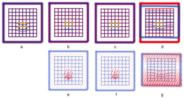
Results of global RBF registration of 3D synthetic images. (a) Overlaid reference (red) and test (blue) images. 6 pairs of corresponding landmarks are indicated by yellow circles and green triangles; (b) result of registration using Gaussian RBF with the radius σ = 50mm; (c) result of registration using Wendland RBF with the radius ρ = 131mm (≈ 2.63 × 50); (d) result of registration using TPS; (e) – (g) deformation vector fields calculated for the cases (b) – (d) correspondingly. The size of the images is 440 × 440 mm. No other registration was used before applying RBF.

It is therefore evident that for problems that require localized deformations, both Gaussian and Wendland functions have an advantage over TPS. The use of TPS in this context requires a uniform landmark distribution throughout the image volume.

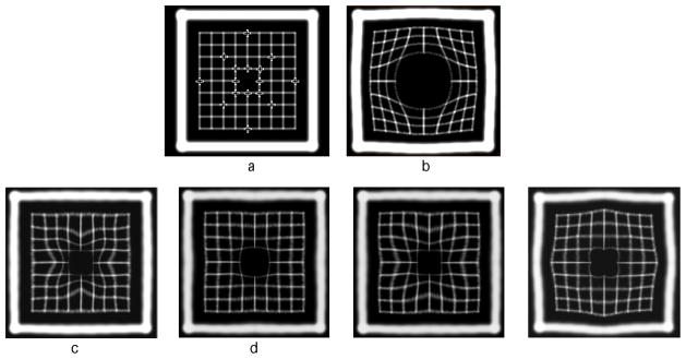
As it is known from the clinical practice, in some cases automatic methods fail to register certain regions within the image. Generally speaking, medical images can be well registered with an intensity-based method on a large scale, but such a method is often unsuccessful at aligning large deformations in areas of fine detail. For example, large changes in position or volume are not generally well aligned for regions with low contrast. Fig. 2 presents cross-sections of synthetic 3-D images that illustrate this problem using a deformation that greatly increases the object volume. This mimics registration of full versus empty bladder or rectum. The automatic B-spline registration does not produce an acceptable result for this case (not shown), i.e. the lattices on the reference and test images do not match, and landmark matching using Gaussian RBF improves the registration result significantly, (see Fig. 2(c)). However, since the volume change is very large, the warped image is stretched unevenly. Regularization improves the smoothness of the deformation field, as it it seen in Fig. 2(d). For comparison we show the results of registration using Wendland RBF (Fig. 2(e)) with the appropriately chosen radius (σ = ρ/2.63) and TPS (Fig. 2(f)). Wendland functions produce the result very similar to the result obtained with Gaussian (cf. Fig. 2(c) and (e)), but the result of regularized Gaussian is superior to both of them. Since the landmarks are distributed evenly across the lattice the image warped with TPS is symmetric (Fig. 2(f)), but has other deficiencies, such as extension of the deformation beyond the fine lattice.

Figure 2.

Results of registration of 3D synthetic images. (a) reference image; (b) test image; (c) registration using 16 landmarks and Gaussian RBF with σ = 38 mm; (d) same as in (c) with regularization; (e) registration using 16 landmarks and Wendland RBF with ρ = 100 mm; (f) registration using 16 landmarks and TPS. The size of the images is 220 × 220 mm.

3.2. Statistical validation of the method

This section is dedicated to validation of our method in statistical terms. We performed a large number of registrations, using the publicly available sets of pulmonary landmarks available from the DIR-Lab web site http://dir-lab.com The dataset consists of 4DCT images, with 300 landmarks manually identified on each image at various time points of the breathing cycle. These large landmark datasets assume rather global registration which is beyond the proposed application of the method but they allow for truly statistics-based conclusions with respect to validity of the method.

In our experiments we evaluate the spatial accuracy of registration on the DIR-Lab data set. Specifically, we compare the performance of the Gaussian RBF with and without regularization to the performance of the Wendland RBF and TPS. To assess the effect of using different numbers of landmarks, we randomly selected M = 1, 2, 4, 6, 8, 10, 15, 25, 50, 75, 100 landmarks out of 300 to be used for registration (“active” landmarks). For each M, 10 different random choices for the set of “active” landmarks were considered. Here, we present the results of the algorithms applied to 5 pairs of images, corresponding to the extreme inhalation and exhalation phases from 4DCT images of 5 different patients. These images are already rigidly aligned, and no coarse registration is required before performing the RBF registration.

It can be expected that specific spatial arrangements of landmarks can cause the Gaussian RBF to produce non-diffeomorphic vector fields, especially for a large number of “active” landmarks. To assess this effect quantitatively, we determine the invertibility of the displacement field. For each image pair and each set of “active” landmarks, we calculate the minimum and maximum value of the determinant of the Jacobian matrix of the field, or simply Jacobian, over the entire voxel volume. Then, for each M, the values of the Jacobian were aggregated over the 10 choices of landmarks and 5 pairs of images.

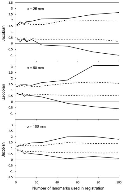
The result of this experiment demonstrates that RBF registration can produce noninvertible transformations in realistic image registration scenarios. In Fig. 3, we show the minimum and maximum values of the Jacobian (solid lines) for three different values of σ. Remarkably, the Jacobian may become negative with as few as 20 landmarks for σ = 25 mm and with about 40 landmarks for σ = 50 mm. For the larger RBF radius of σ = 100 mm the Jacobian remained positive. From this result, we conclude that Gaussian RBF-based registrations can indeed contain singularities and non-invertible areas. The same experiment was then repeated using registration with regularization (λ = 0.1). In this case the Jacobian was strictly positive over the entire image volume for all image pairs and all sets of active landmarks (see dashed lines in Fig. 3). Therefore, regularization of the RBF vector field is necessary, and our method provides it in the familiar RBF linear equations framework, ensuring computational efficiency.

Figure 3.

Minimum and maximum values of the Jacobian of the test-to-reference image transformation as a function of the number of landmark pairs used for Gaussian RBF field calculations. Different values of σ are tested on 5 sets of images acquired form 5 different patients. Solid lines are the results for registration without regularization, dashed lines are for registration with regularization (λ = 0.1).

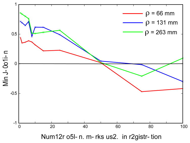
To investigate the invertibility of deformation field produced by the Wendland function, we calculated the minimum value of Jacobian following the same procedure as for the Gaussian (see above). Fig. 4 demonstrates that the deformation field becomes non-invertible at large number of landmarks for any choice of theWendland RBF radius. Therefore, we conclude that despite the fact that the Wendland functions are more efficient computationally than the Gaussian, they too require regularization to avoid non-invertibility of the resulting field. However, we are not aware of an exact expression for regularizing Wendland RBF, and it is very likely that it does not exist due to their finite support.

Figure 4.

Minimum values of the Jacobian of the test-to-reference image transformation as a function of the number of landmark pairs used for Wendland RBF field calculations. Different values of ρ are tested on 5 sets of images acquired from 5 different patients.

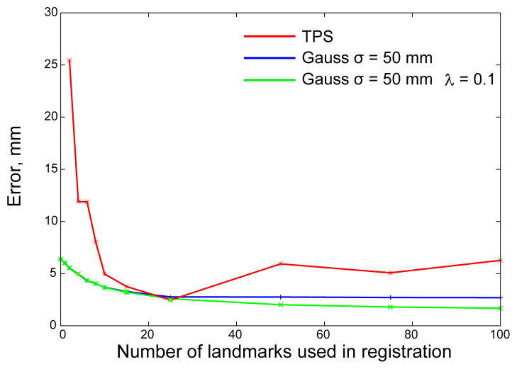
To quantify the accuracy of registration, in Fig. 5 we plot the registration error (the average residual distance between the 300 − M “passive” landmarks on the reference and warped images) as function of the number of “active” landmarks M. The case of M = 0 corresponds to unregistered images with the error reported in the original papers (Castillo E et al 2009, Castillo R et al 2009).

Figure 5.

Registration error as a function of the number of landmark pairs used in RBF field calculations. Different algorithms are tested on 5 sets of images acquired form 5 different patients. The result for non-regularized Gaussian RBF with σ = 50 mm is shown in blue and for regularized Gaussian RBF with σ = 50 and λ = 0.1 is shown in green; result for TPS is shown in red.

Fig. 5 shows that registration accuracy improves as more landmarks are used for registration. If the number of landmarks is less than about 20, either regularized Gaussian or non-regularized functions produce identical results. As the number of landmarks increases, the accuracy of registration becomes different for the two settings. For this dataset, the accuracy is best if one uses Gaussian RBF with regularization, but both regularized and non-regularized Gaussian functions outperform TPS. The large TPS registration error for a small number of landmarks is expected, since the method is designed for global registration with landmarks uniformly distributed in 3D. The error becomes lower with increasing number of landmarks and at M ≈ 25 performances of Gaussian function and TPS are comparable. Interestingly, at larger M, the TPS performance decreases again. For the small numbers of landmarks, expected in the daily clinical applications, the performance of our method (3.6 mm average registration error for 10 landmarks) is close to the goal of 3 mm stated in the Introduction.

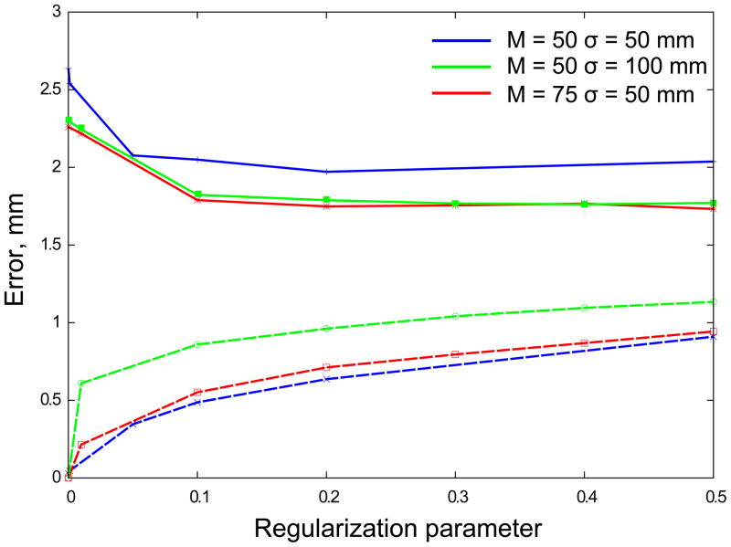
Since regularization involves a trade off between precision of landmarks matching and smoothness of the vector field, the limits for the regularization parameter λ have to be established. In Fig. 6 we plot the registration error and distance between “active” landmarks as a function of the parameter λ. Indeed, increasing λ improves registration accuracy (see Fig. 6, solid lines) and worsens the landmark matching (Fig. 6, dashed lines). Both quantities plateau at λ ≈ 0.2 that is the best choice for the regularization parameter for these images. As more landmarks and larger RBF radii are used, the regularization becomes more effective and larger values of λ can be used without degrading the matching accuracy.

Figure 6.

Registration error as a function of regularization parameter, λ. Different parameters are tested on 5 sets of images acquired form 5 different patients. Blue lines: number of “active” landmarks M = 50 and σ = 50 mm; green lines: M = 50 and σ = 100; red lines: M = 75 and σ = 50. The distances between “passive” landmarks (accuracy of registration) are shown by solid lines, the distances between “active” landmarks (mismatch error) are shown by dashed lines.

In summary, we have established that the regularized Gaussian RBF consistently produce better registration accuracy at large number of landmarks (see Fig. 5), and that they can achieve invertible deformation fields. We believe that regularization reduces the registration error because the displacement field is smoother, and more closely matches the smooth anatomic change found in the pulmonary images.

3.3. Application to clinical images

Having validated our method in statistical terms, we will now present representative results of registration of clinical case images.

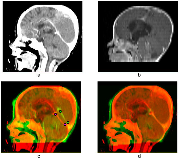
The following examples will demonstrate the usefulness of our landmark-based RBF method as a method for enhancing automatic registration based on a B-spline approximation algorithm (Sharp et al. 2010). Fig. 7 illustrates a case with poor registration. Brain images were acquired from different modalities at different times: the reference image is the CT of 2-year old patient (Fig. 7(a)) and test image is the MRI of the same patient at 6 months of age (Fig. 7(b)). By using the automatic B-spline registration we obtain an image with a properly aligned and sized skull but misaligned intra-cranial features (see Fig. 7(c)). To correct the registration we marked two landmarks on the superior boundary of the cerebellum (shown in Fig. 7(c)) and calculate the RBF field. The combination of both vector fields results in reasonably good alignment of the feature of interest (Fig. 7(d)). In this case, corrections to the B-spline registration used only a few, localized landmarks, so we did not have to use regularization.

Figure 7.

(a) Reference image (CT); (b) test image (MRI); (c) result of automatic B-spline registration of the MRI image onto the CT image; (d) B-spline algorithm and subsequent application of Gaussian RBF with σ = 35 mm for landmark matching.

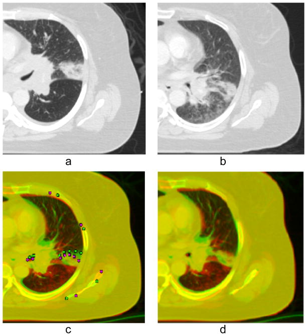
In a more complicated case, Fig. 8(a) shows a pre-treatment radiotherapy planning CT of a patient being treated for small-cell lung cancer with a curative dose of radiotherapy, delivered fractionally over the course of six weeks. After three weeks of treatment, the patient received a second CT scan, shown in Fig. 8(b), which demonstrates a significant response to treatment as well as a posterior shift in the position of the tumor by about 2 cm. At this point, the physician alters the radiotherapy beam geometry to match the new position of the tumor, and requests a composite dose distribution that aggregates the dose delivered to the anatomy seen in 8(a) and (b). Deformable image registration is performed using an automatic B-spline approximation algorithm (Sharp et al. 2010), but only about 1 cm of the tumor shift is recovered (Fig. 8(c)). The remaining 1 cm of the tumor shift is recovered by placing five pairs of corresponding landmarks along tumor boundary. In addition we placed landmarks to recover positions of the left shoulder blade, the aorta, and ribs. A total of 11 landmarks were used on a single axial slice (see Fig. 8(c) where landmarks in the reference image are shown in pink and landmarks in the test image, obtained after B-spline registration, are shown in green). Since many distant landmarks are involved in RBF field calculation, the regularization term will assure a smooth resulting field without unwanted foldings in the space between landmarks. The final result of registration with composed B-spline and RBF vector fields is shown in Fig. 8(d). While the accuracy of registration cannot be measured as rigorously as in DIR-lab data, visual examination of Fig. 8 and 7 suggests that our algorithm meets the desired performance of 3 mm landmark position error.

Figure 8.

Results of registration of two CT images of the lung obtained before and during treatment. (a) The image obtained before treatment (test image); (b) the image obtained during treatment (reference image); (c) result of automatic B-spline registration of the test image onto the reference image, 11 pairs of landmarks are placed in the referenced and warped by B-spline images; (d) result of registration by B-spline algorithm and subsequent application of Gaussian RBF with σ = 15 mm and λ = 0.1 for landmark matching.

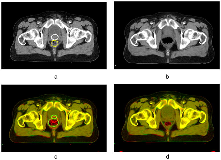
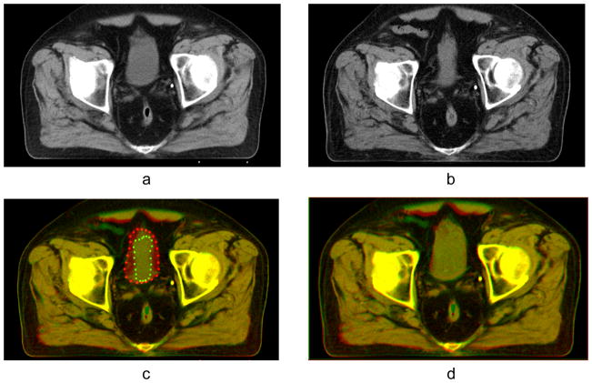
Even more complicated deformations involving large volumeric changes are presented in Figs. 9 and 10. Here, we applied our method to register CT images of the prostate acquired at different days during radiation treatment. Fig. 9 represents a case with a largely deformed rectum and Fig. 10 is a typical example of full vs empty bladder registration. In both cases the change in size of the rectum or the bladder is not captured correctly by automatic registration using B-splines (see Figs. 9(c) and 10(c)). Accurate registration is, however, highly desirable since in these cases the deformations of adjacent organs influences the position of prostate and may cause it to shift out of the radiation field.

Figure 9.

(a) Reference image with empty rectum, the landmarks are place along the contours of prostate (white) and rectum (yellow); (b) test image with full rectum; (c) result of automatic B-spline registration of the test image onto the reference image, mismatched contours of landmarks are shown in red and green; (d) result of registration by B-spline algorithm and subsequent application of Gaussian RBF with σ = 10 mm and λ = 0.5 for landmark matching.

Figure 10.

(a) Reference image with full bladder; (b) test image with empty bladder; (c) result of automatic B-spline registration of the test image onto the reference image, mismatched contours of landmarks are shown in red and green; (d) result of registration by B-spline algorithm and subsequent application of Gaussian RBF with σ = 15 mm and λ = 0.7 for landmark matching.

Landmarks were placed on the prostate, rectum, and bladder using the radiotherapy planning structures. Each contour was fit to an ellipse, and the landmarks were then evenly distributed along the contour boundary with radially equal spacing. In Fig. 9(a) one can see the landmarks placed along the contours of the rectum (yellow) and prostate (white) in the reference image. The test image with enlarged rectum (Fig. 9(b)) is registered with the reference image. B-spline automatic registration does not produce an acceptable result for this case (see Fig. 9(c)). To correct the automatic registration we used landmarks along the contours in the reference image and the image warped with B-splines by applying the deformation field build on RBFs. Since the decrease in volume of the rectum was very large, the deformation field was regularized to assure diffeomorphism of the deformation. As one can see, the application of our landmark matching algorithm significantly improves the quality of registration (see Fig. 9(d)).

Figure 10 demonstrates a correction of the automatic registration of the bladder. In this case the size of a full bladder in the reference image is considerably larger than the size of an empty bladder in the test image, which causes misalignment of the structure after B-spline registration (see Fig. 10(c)). After registration with the RBF, the empty bladder is well aligned with the full bladder as seen in Fig. 10(d). The regularization term ensures deffeomorphism of the deformation.

To assess an accuracy of the registration quantitatively, we calculated the Dice similarity coefficient (DSC) (Dice 1945) between manually identified contours on the reference image and the contours propagated onto warped image using different modes of registration. As shown in Table 2, the structures remain misaligned after rigid as well as B-spline transformation, whereas registration with regularized RBF field results in nearly perfect alignment. Use of RBF field without regularization does not improve, but sometimes even worsens the registration because of vector field folding. This is illustrated in Fig. 11 where we show the contour of the bladder obtained by warping the contour with the vector field obtained by composing the B-spline vector field and RBF vector field. A smooth contour in Fig. 11(a) corresponds to the regularized RBF vector field and irregular contour in Fig. 11(b) is a result of a non-regularized field.

Table 2.

Dice coefficient (DSC) for the contours of the structures shown in Figs. 9 and 10

Transformation to warp	DSC	DSC
	Rectum	Prostate
rigid	0.56	0.53
B-spline	0.61	0.59
RBF without regularization	0.54	0.86
RBF with regularization	0.9	0.91
	Bladder	Prostate
rigid	0.56	0.80
B-spline	0.64	0.80
RBF without regularization	0.70	0.62
RBF with regularization	0.87	0.92

Figure 11.

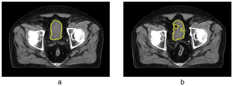
Result of registration of the bladder and contour propagation with composed B-spline and RBF vector field (a) with regularization; (b) without regularization.

4. Discussion

The contribution of this paper is the introduction of a fast, exact algorithm for a regularized vector field from Gaussian RBFs. Our algorithm is exact in the sense that the regularization term is evaluated analytically, and represents a bilinear form in terms of RBF coefficients. The algorithm is fast, since the the RBF coefficients α_ij are found by solving a system of linear equations (12), rather than by gradient descent minimization. We anticipate that the key practical application of the algorithm will be to correct imprecise automatic registration results, or enhance the registration results in areas of low contrast.

One important property of the Gaussian basis is its infinite support. It has been argued (Arad and Reisfeld 1995, Fornefett et al 2001) that infinite support is not desirable, because each landmark pair affects the field at every voxel. In contrast, RBFs with local support can ensure that the extra deformation due to landmarks is exactly zero beyond the radius of support of the function. Furthermore, an RBF with compact support can be interpolated very quickly, because each RBF influences relatively fewer voxels. The computational advantage of the Gaussian RBF comes from the ability to calculate the regularization term analytically. Unfortunately, analytical calculation of the second-derivative integrals for an arbitrary number of overlapping Wendland functions is not feasible, as it is impossible to predict the shape of the intersection of multiple compact supports.

It is interesting to compare our scheme to that of Rohr et al. (Rohr et al 2001), which introduces the notion of landmark localization error. Rohr et al. argues that since the positions of landmarks are not precisely known, it is unnecessary to exactly match the landmarks, especially where this creates strong gradients of the deformation field. Accordingly, their cost function consists of two terms, the usual TPS bending energy, and the sum of Euclidean distances between the landmarks, weighted by the “radius of uncertainty” in landmark location. As in our case, minimization leads to a system of linear equations, and the resulting vector field is a tradeoff between smoothness and exactness of landmark matching. However, there are fundamental differences between our approach and that of Rohr et al. In our case, the radius of influence of each RBF is explicitly controlled by choosing the width σ of the Gaussian function. Amplitudes of each RBF are then found to balance between good landmark matching and smoothness of the vector field. In the Rohr et al. algorithm, the basis functions are the TPS, with infinite support and no control parameter for the radius of influence. The minimization procedure should then result in decreased amplitudes of the TPS centered on landmarks whose positions are poorly known, to minimize the contribution of ill-defined landmarks to the vector filed.

Having an explicit parameter σ to control the radius of influence of point landmarks is an advantage of our method. While both methods produce a regularized vector field by solving a system of linear equations, there is no guarantee that suppressing the TPS amplitude would confine the influence of a particular landmark to a well-defined area. It is also not very clear how one would determine the relative landmark localization errors that match an interactive user’s expectations. In contrast, our approach provides the user with two control parameters, σ and λ one of which has the obvious meaning of the RBF radius, and the other is a control for smoothness. As presented here, our algorithm assumes that all landmarks have the same (zero) landmark localization error. An error term could be easily incorporated, by appropriately weighting the squared distances terms in 8, just as in (Rohr et al 2001). Such an extension would preserve the structure of all the equations, and so would not result in any speed or memory penalty. However, considerable effort will be required to develop the methods of estimating landmark localization errors for each medical application.

Our method of regularization of the RBF-based vector fields is completely general in the sense that it can be applied to any RBF with infinite support. The calculation of the regularization matrix A_ij for the Gaussian RBF, presented in the Appendix, can be repeated for other choices of RBF given that they are infinite in space. In the case where the integrals are too cumbersome or impossible to evaluate exactly, they can be approximated numerically. Since this should be done only once for a given type and radius of RBF, registration of large numbers of images is very fast as compared to any numerical minimization procedure, because it requires only to solve the system of 3M linear equations (9) for each pair of test and reference images.

Invertibility of the registration transformation requires its Jacobian to maintain the same sign (usually positive) within the image, and we have shown experimentally that RBF-built displacement fields are usually invertible. At present, we are not aware of any analytic method to incorporate constraints on the Jacobian in the RBF registration. The Jacobian is trilinear in 3D, rather than bilinear, with respect to the coefficients α_ip, which makes it hard, if not impossible, to constrain while obtaining the RBF coefficients α_ip from a system of linear equations. However, we demonstrate that a penalty on the square of second derivatives of the displacement field can produce smooth and invertible fields while being very efficient computationally.

5. Conclusions

We have developed a practical method for correction and repair of automatic image registration results. In the intended clinical application, misregistered regions are visually identified, landmarks are manually placed, and the algorithm will produce a correcting vector field with several highly desirable properties. First, due to the choice of Gaussian RBFs, the corrections will be localized to misregistered areas, given that the Gaussian width is chosen accordingly to the desired extent of the correction. Second, since the vector field is regularized, it is easy to achieve the invertibility and smoothness of the transformation. Importantly, our technique employs a novel analytic regularization method, which does not require gradient descent or other numerical optimization, but calculates the RBF coefficients for a regularized vector field by solving the system of linear equations. Therefore, our method is highly computationally efficient, can be generalized to any type of RBF with infinite support, and easily incorporates into existing software.

Using large, publicly available datasets, we statistically validated our method, and showed the importance of regularization when registering images with large numbers of landmarks. The performance of the method was close to a clinically desirable goal of 3 mm error in landmark position. Furthermore, we provide clinical examples of brain, lung, prostate and rectum images, where our method has successfully repaired automatic B-spline registrations. We hope that our general analytic scheme of RBF regularization will prove useful in other contexts of medical image registration.

Appendix

The displacement value of the deformation field along x-axis (x-component of the deformation field) at a position r⃗ is given by a linear combination of radial basis functions:

$$u_x(\overrightarrow{r})=\sum _{i=1}^M{\alpha }_{ix}\psi (||\overrightarrow{r}-{\overrightarrow{r}}_{Ri}||),$$ (A.1)

where r⃗_Ri is a position of ith landmark on the reference image. To evaluate the regularization term, (5), we substitute (A.1) into (5). Note that (5) conveniently splits into a sum of second-order partial derivatives and mixed partial derivatives, which can be evaluated separately. Furthermore, we can interchange the order of summation over the RBFs in (A.1) and summation (integration) over the entire volume in (5).

To simplify notation, let us introduce the distance vector between two landmarks a⃗_ij as

$${\overrightarrow{a}}_{ij}={\overrightarrow{r}}_{Ri}-{\overrightarrow{r}}_{Rj}=a_x{\overrightarrow{e}}_x+a_y{\overrightarrow{e}}_y+a_z{\overrightarrow{e}}_z,$$ (A.2)

and the distances ρ = |ρ⃗|, ρ_i = |r⃗ − r⃗_i|, ρ_j = |r⃗ − r⃗_j|, and finally ρ_aij = |r⃗ − a⃗_ij|.

Then, the second-order partial derivative term consists of two parts, one of which (I₁) depends only on RBF shape, and the other (I₂) depends also on the distances between pairs of landmarks a_ij (A.3):

$$\begin{array}{l}\sum _{i,j=1}^M{\alpha }_{ix}{\alpha }_{jx}\underset{-\infty }{\overset{\infty }{\int }}\left[{\psi }_{xx}^{″}({\rho }_i){\psi }_{xx}^{″}({\rho }_j)+{\psi }_{yy}^{″}({\rho }_i){\psi }_{yy}^{″}({\rho }_j)+{\psi }_{zz}^{″}({\rho }_i){\psi }_{zz}^{″}({\rho }_j)\right]\mathit{dxdydz}\\ =\sum _{i=1}^M{\alpha }_{ix}^2\underset{-\infty }{\overset{\infty }{\int }}\left[{({\psi }_{xx}^{″}(\rho ))}^2+{\left({\psi }_{yy}^{″}(\rho )\right)}^2+{({\psi }_{zz}^{″}(\rho ))}^2\right]\mathit{dxdydz}\\ +2\sum _{i\ne j}^M{\alpha }_{ix}{\alpha }_{jx}\underset{-\infty }{\overset{\infty }{\int }}\left[{\psi }_{xx}^{″}(\rho ){\psi }_{xx}^{″}({\rho }_{a_{ij}})+{\psi }_{yy}^{″}(\rho ){\psi }_{yy}^{″}({\rho }_{a_{ij}})+{\psi }_{zz}^{″}(\rho ){\psi }_{zz}^{″}({\rho }_{a_{ij}})\right]\mathit{dxdydz}\\ =3I_1\sum _{i=1}^M{a}_{ix}^2+2\sum _{i\ne j}^M{a}_{ix}{a}_{jx}(I_{2,xx}+I_{2,yy}+I_{2,zz}).\end{array}$$ (A.3)

Similarly, the mixed partial derivatives read

$$\begin{array}{l}\sum _{i=1}^M{\alpha }_{ix}^2\underset{-\infty }{\overset{\infty }{\int }}\left[{\left({\psi }_{xy}^{″}(\rho )\right)}^2+{\left({\psi }_{yz}^{″}(\rho )\right)}^2{({\psi }_{xz}^{″}(\rho ))}^2\right]\mathit{dxdydz}\\ +2\sum _{i\ne j}^M{\alpha }_{ix}{\alpha }_{jx}\underset{-\infty }{\overset{\infty }{\int }}\left[{\psi }_{xy}^{″}(\rho ){\psi }_{xy}^{″}({\rho }_{a_{ij}})+{\psi }_{yz}^{″}(\rho ){\psi }_{yz}^{″}({\rho }_{a_{ij}})+{\psi }_{xz}^{″}(\rho ){\psi }_{xz}^{″}({\rho }_{a_{ij}})\right]\mathit{dxdydz}\\ =3I_3\sum _{i=1}^M{a}_{ix}^2+2\sum _{i\ne j}^M{a}_{ix}{a}_{jx}(I_{4,xy}+I_{4,yz}+I_{4,xz}).\end{array}$$ (A.4)

Up to this point our expressions are general. For the Gaussian function

$$\psi (|\left|\overrightarrow{r}\right||)=\psi (r)=e^{-r^2/{\sigma }^2},r=\sqrt{x^2+y^2+z^2}$$ (A.5)

we obtain

$$\frac{{\partial }^2\psi }{\partial x^2}=\left[-\frac{2}{{\sigma }^2}+\frac{4x^2}{{\sigma }^4}\right]e^{-r^2/{\sigma }^2},$$ (A.6)

so

$${\left(\frac{{\partial }^2\psi }{\partial x^2}\right)}^2=\left[\frac{4}{{\sigma }^4}-\frac{16x^2}{{\sigma }^6}+\frac{16x^4}{{\sigma }^8}\right]e^{-2r^2/{\sigma }^2}.$$ (A.7)

The Integrals I₁ and I₂ in (A.3) are written as follows:

$$I_1={\int }_{-\infty }^{\infty }{e}^{-2r^2/{\sigma }^2}\left[\frac{4}{{\sigma }^4}-\frac{16x^2}{{\sigma }^6}+\frac{16x^4}{{\sigma }^8}\right]d\overrightarrow{r}$$ (A.8)

and

$$I_{2,xx}={\int }_{-\infty }^{\infty }\frac{{\partial }^2\psi (|\left|\overrightarrow{r}\right||)}{\partial x^2}\frac{{\partial }^2\psi (||\overrightarrow{r}-{\overline{a}}_{ij}||)}{\partial x^2}d\overrightarrow{r}.$$ (A.9)

Using the integrals

$${\int }_{-\infty }^{\infty }{e}^{-2r^2/{\sigma }^2}d\overrightarrow{r}={\left({\int }_{-\infty }^{\infty }{e}^{-2x^2/{\sigma }^2}dx\right)}^3={\left(\sigma \sqrt{\frac{\pi }{2}}\right)}^3,$$ (A.10)

$${\int }_{-\infty }^{\infty }{x}^2{e}^{-2r^2/{\sigma }^2}d\overrightarrow{r}={\left(\sigma \sqrt{\frac{\pi }{2}}\right)}^2=\left(\frac{1}{4}{\sigma }^3\sqrt{\frac{\pi }{2}}\right),$$ (A.11)

$${\int }_{-\infty }^{\infty }{x}^4{e}^{-2r^2/{\sigma }^2}d\overrightarrow{r}={\left(\sigma \sqrt{\frac{\pi }{2}}\right)}^2\left(\frac{3}{16}{\sigma }^5\sqrt{\frac{\pi }{2}}\right),$$ (A.12)

we obtain the following result for I₁:

$$I_1=\frac{3}{\sigma }{\left(\frac{\pi }{2}\right)}^{3/2}\equiv 3\kappa .$$ (A.13)

Calculation of I_2,xx is very similar, as (A.9) can be rewritten

$$I_{2,xx}={\int }_{-\infty }^{\infty }\left[-\frac{2}{{\sigma }^2}+\frac{4x^2}{{\sigma }^4}\right]\left[-\frac{2}{{\sigma }^2}+\frac{4{(x-a_x)}^2}{{\sigma }^4}\right]\times e^{-\frac{x^2+{(x-a_x)}^2}{{\sigma }^2}}{e}^{-\frac{y^2+{(y-a_y)}^2}{{\sigma }^2}}{e}^{-\frac{x^2+{(z-a_z)}^2}{{\sigma }^2}}d\overrightarrow{r}$$ (A.14)

After the change of variables u = x − a_x/2 and factorization we obtain

$$\begin{array}{l}{I}_{2,xx}=\{\left[\frac{4}{{\sigma }^4}-\frac{4a_x^2}{{\sigma }^6}+\frac{a_x^4}{{\sigma }^8}\right]{\int }_{-\infty }^{\infty }{e}^{-2u^2/{\sigma }^2}du\\ +\left[-\frac{4}{{\sigma }^6}+\frac{2a_x^2}{{\sigma }^8}\right]{\int }_{-\infty }^{\infty }{u}^2{e}^{-2u^2/{\sigma }^2}du\\ +\frac{16}{{\sigma }^8}{\int }_{-\infty }^{\infty }{u}^4{e}^{-2u^2/{\sigma }^2}du\}\times e^{-a/2{\sigma }^2}{\left({\int }_{-\infty }^{\infty }{e}^{-2u^2/{\sigma }^2}du\right)}^2\\ =\kappa e^{-a^2/2{\sigma }^2}\left[3-\frac{6a_x^2}{{\sigma }^2}+\frac{a_x^4}{{\sigma }^4}\right],\end{array}$$ (A.15)

where a ≡ ||a_ij|| is the distance between landmarks i and j. Thus, the sum I_2,xx + I_2,yy + I_2,zz is equal to

$$\kappa e^{-a^2/2{\sigma }^2}\left[9-\frac{6}{{\sigma }^2}\left(a_x^2+a_y^2+a_z^2\right)+\frac{1}{{\sigma }^4}\left(a_x^4+a_y^4+a_z^4\right)\right].$$ (A.16)

The sum of mixed partial derivatives also splits into two parts (14).

For the Gaussian function the mixed partial derivative reads

$$\frac{{\partial }^2\psi }{\partial x\partial y}=\frac{4xy}{{\sigma }^4}{e}^{-r^2/{\sigma }^2},$$ (A.17)

so

$$I_3=\frac{16}{{\sigma }^8}{\int }_{-\infty }^{\infty }{e}^{-2z^2/{\sigma }^2}dz{\int }_{-\infty }^{\infty }{x}^2{y}^2{e}^{-2(x^2+y^2)/{\sigma }^2}\mathit{dxdy}.$$ (A.18)

Using polar coordinates for the second integral in (A.18) we get

$${\int }_0^{2\pi }{cos}^2\varphi {sin}^2\varphi d\varphi {\int }_0^{\infty }{r}^5{e}^{-2r^2/{\sigma }^2}dr=\frac{\pi }{4}\frac{{\sigma }^6}{8},$$ (A.19)

so

$$I_3=\kappa .$$ (A.20)

The fourth type of integrals can be evaluated in a similar fashion:

$$I_{4,xy}=\frac{16}{{\sigma }^8}{\int }_{-\infty }^{\infty }xy(x-a_x)(y-a_y)e^{-\frac{{\overrightarrow{r}}^2+{(\overrightarrow{r}-{\overrightarrow{a}}_{ij})}^2}{{\sigma }^2}}d\overrightarrow{r}$$ (A.21)

After change of variables one has to evaluate the integral

$${\int }_{-\infty }^{\infty }\left(u^2-\frac{a_x^2}{4}\right)\left(v^2-\frac{a_y^2}{4}\right)e^{-2(u^2+v^2)/{\sigma }^2}\mathit{dudv}$$ (A.22)

and obtain the result

$$I_{4,xy}=\kappa e^{-a^2/2{\sigma }^2}\left[1-\frac{a_x^2+a_y^2}{{\sigma }^2}+\frac{a_x^2{a}_y^2}{{\sigma }^4}\right].$$ (A.23)

Using Eqs. (A.13, A.15, A.20, A.23), we finally obtain

$$\begin{array}{l}{G}_{\mathit{reg}}=3\sum _{i=1}^M{\alpha }_{ix}^2{I}_1+2\sum _{i\ne j}^M{\alpha }_{ix}{\alpha }_{jx}(I_{2,xx}+I_{2,yy}+I_{2,zz})+6\sum _{i=1}^M{\alpha }_{ix}^2{I}_3+4\sum _{i\ne j}^M{\alpha }_{ix}{\alpha }_{jx}(I_{4,xy}+I_{4,yz}+I_{4,xz})\\ =\kappa \left[15\sum _{i=1}^M{\alpha }_{ix}^2+2\sum _{i\ne j}^M{\alpha }_{ix}{\alpha }_{jx}{e}^{-a^2/2{\sigma }^2}\left(15-\frac{10a^2}{{\sigma }^2}+\frac{a^4}{{\sigma }^4}\right)\right].\end{array}$$ (A.24)

The latter expression can be factorized, and after adding y- and z-components we arrive at the equation (6) (up to a constant factor).

References

- Arad N, Dyn N, Reisfeld D, Yeshurun Y. Image warping by radial basis functions: application to facial expression. CVGIP: Graph Models Image Processing. 1994;56:161–72. [Google Scholar]
- Arad N, Reisfeld D. Image warping using few anchor points and radial functions. Computer Graphics Forum. 1995;14:35–46. [Google Scholar]
- Boldea V, Sharp GC, Jiang SB, Sarrut D. 4D-CT lung motion estimation with deformable registration: quantification of motion nonlinearity and hysteresis. Med Phys. 2008;35:1008–18. doi: 10.1118/1.2839103. [DOI] [PubMed] [Google Scholar]
- Bookstein FL. Principal warps: thin-plate splines and the decomposition of deformations. IEEE Trans Pattern Anal Machine Intell. 1989;11:567–85. [Google Scholar]
- Buhmann MD. Radial basis functions. Acta Numerica. 2000;9:1–38. [Google Scholar]
- Cao K, Du K, Ding K, Reinhardt JM, Christensen GE. Regularized nonrigid reistration of lung CT images by preserving tissue volume and vesselness measure: The EMPIRE10 study. In: van Ginneken B, Murphy K, Heimann T, pekar V, Deng X, editors. Medical image analysis for the clinic: a grand challenge 2010. Beijing: China Workshop Proceedings; 2010. p. 43. [Google Scholar]
- Castillo E, Castillo R, Guerra R, Zhang Y, Guerrero T. Compressible image registration for thoracic computed tomography images. J Med Biol Eng. 2009;29:222–33. [Google Scholar]
- Castillo R, Castillo E, Guerra R, Johnson VE, McPhail T, Garg AK, Guerrero T. A Framework for evaluation of deformable image registration spatial accuracy using large landmark point sets. Phys Med Biol. 2009;54:1849–70. doi: 10.1088/0031-9155/54/7/001. [DOI] [PubMed] [Google Scholar]
- Christensen GE, Rabbitt RD, Miller MI. Deformable templates using large deformation kinematics. IEEE Trans Image Process. 1996;5:1435–47. doi: 10.1109/83.536892. [DOI] [PubMed] [Google Scholar]
- Christensen GE, Joshi SC, Miller MI. Volumeric transformation of brain anatomy. IEEE Trans Med Imag. 1997;16:864–77. doi: 10.1109/42.650882. [DOI] [PubMed] [Google Scholar]
- Dice LR. Measures of the amount of ecologic association between species. Ecology. 1945;26:297–302. [Google Scholar]
- Fornefett M, Rohr K, Stiehl HS. Radial basis functions with compact support for elastic registration of medical images. Img Vis Comp. 2001;19:87–96. [Google Scholar]
- Han X. Feature-constrained nonlinear registration of lung CT images: The EMPIRE10 study. In: van Ginneken B, Murphy K, Heimann T, pekar V, Deng X, editors. Medical image analysis for the clinic: a grand challenge 2010. Beijing: China Workshop Proceedings; 2010. p. 63. [Google Scholar]
- Holden M. A review of geometric transformations for nonrigid body registration. IEEE Trans Med Imag. 2008;27:111–28. doi: 10.1109/TMI.2007.904691. [DOI] [PubMed] [Google Scholar]
- Johnson H, Christensen G. Consistent Landmark and intensity based image registration. IEEE Trans Med Imag. 2002;21:450–61. doi: 10.1109/TMI.2002.1009381. [DOI] [PubMed] [Google Scholar]
- Klein EE, Hanley J, Bayouth J, Yin F-F, Simon W, Dresser S, Serago C, Aguirre F, Ma L, Arjomandy B, Liu C. Task Group 142 report: Quality assurance of medical accelerators. Med Phys. 2009;36:4197–4212. doi: 10.1118/1.3190392. [DOI] [PubMed] [Google Scholar]
- Kohlrausch J, Rohr K, Stiehl HS. A new class of elastic body splines for nonrigid registration of medical images. J Math Imag Vis. 2005;23:253–80. [Google Scholar]
- Kybic J, Unser M. Fast parametric elastic image registration. IEEE Trans Imag Proc. 12:1427–42. doi: 10.1109/TIP.2003.813139. [DOI] [PubMed] [Google Scholar]
- Lester H, Arridge SR. A survey of hierarchical non-linear medical image registration. Pattern Recognition. 1999;32:129–49. [Google Scholar]
- Loeckx D, Smeets D, Keustermans J, Hermans J, Maes F, Vandermeulen D, Suetens P. 3D Lung registration using splineMIRIT and robust tree registration (RTR): The EMPIRE10 study. In: van Ginneken B, Murphy K, Heimann T, pekar V, Deng X, editors. Medical image analysis for the clinic: a grand challenge 2010. Beijing: China Workshop Proceedings; 2010. p. 109. [Google Scholar]
- Murphy K, van Ginneken B, Reinhardt JM, Kabus S, Ding K, Deng X, Pluim JPW. Evaluation of methods for pulmonary image registration: The EMPIRE10 study. In: van Ginneken B, Murphy K, Heimann T, pekar V, Deng X, editors. Medical image analysis for the clinic: a grand challenge 2010. Beijing: China Workshop Proceedings; 2010. p. 11. [Google Scholar]
- Pekar V, Gladilin E, Rohr K. An adaptive irregular grid approach for 3D deformable image registration. Phys Med Biol. 2006;51:361–77. doi: 10.1088/0031-9155/51/2/012. [DOI] [PubMed] [Google Scholar]
- Rohr K, Stiehl HS, Sprengel R, Buzug TM, Weese J, Kuhn MH. Landmark-based elastic registration using approximating thin-plate splines. IEEE Trans Med Imag. 2001;20:526–34. doi: 10.1109/42.929618. [DOI] [PubMed] [Google Scholar]
- Rohr K, Cathier P, Worz S. Elastic registration of electrophoresis images using intensity information and point landmarks. Pattern Recogn. 2004;37:1035–48. [Google Scholar]
- Rueckert D, Sonoda LI, Hayes C, Hill DLG, Leach MO, Hawkes DJ. Nonrigid registration using free-form deformations: application to breast MR images. IEEE Trans Med Imag. 18:712–21. doi: 10.1109/42.796284. [DOI] [PubMed] [Google Scholar]
- Rohlfing T, Maurer CR, Jr, Bluemke DA, Jacobs MA. Volume-preserving nonrigid registration of MR breast images using free-form deformation with an incompressibility constraint. IEEE Trans Med Imaging. 22:730–41. doi: 10.1109/TMI.2003.814791. [DOI] [PubMed] [Google Scholar]
- Sorzano COS, Thevenaz P, Unser M. Elastic registration of biological images using vector-spline regularization. IEEE Trans Biomed Eng. 52:652–63. doi: 10.1109/TBME.2005.844030. [DOI] [PubMed] [Google Scholar]
- Sharp GC, Lui R, Wolfgang J, Chen GTY, Peroni M, Spadea MF, Mori S, Zhang J, Shackleford J, Kandasamy N. Plastimatch an open source software suite for radiotherapy image processing. Proc. 16th Int. Conf. on the Use of Computers in Radiotherapy (ICCR); Amsterdam. 2010. [Google Scholar]
- Unser M, Aldroubi A, Eden M. Fast b-spline transforms for continuous image representation and interpolation. IEEE Trans Pattern Anal Mach Intell. 1991;13:277–85. [Google Scholar]
- Unser1Unser M. Splines: A perfect fit for signal and image processing. IEEE Signal Process Magazine. 1999;16:22–38. [Google Scholar]
- Wörz S, Rohr K. Physics-based elastic registration using non-radial basis functions and including landmark localization uncertainties. Comp Vis Image Underst. 2008;111:263–74. doi: 10.1007/11866763_83. [DOI] [PubMed] [Google Scholar]
- Zitova B, Flusser J. Image registration methods: a survey. Img Vis Comp. 2003;21:977–1000. [Google Scholar]