Why the Items versus Parcels Controversy Needn’t Be One

Abstract

The use of item parcels has been a matter of debate since the earliest use of factor analysis and structural equation modeling. Here, we review the arguments that have been levied both for and against the use of parcels, and discuss the relevance of these arguments in light of the building body of empirical evidence investigating their performance. We discuss the many advantages of parcels that some researchers find attractive and highlight, too, the potential problems that ill-informed use can incur. We argue that no absolute pro or con stance is warranted. Parcels are an analytic tool like any other. There are circumstances in which parceling is useful and times when parcels would not be used. We emphasize the precautions that should be taken when creating item parcels and interpreting model results based on parcels. Finally, we review and compare several proposed strategies for parcel building, and suggest directions for further research.

Since the earliest use of factor analysis, controversy has surrounded the use of item parcels as indicators of latent factors. This debate has arisen in the contexts of exploratory factor analysis, confirmatory factor analysis, and structural equation modeling. In this paper, we argue that there is now sufficient evidence about the behavior of parcels that the items versus parcels controversy needn’t remain a controversy.¹ We begin our discussion with a premise that we support below: Parcels, per se, are not inaccurate, incorrect, or faulty. When thoughtfully composed, parcels provide efficient, reliable, and valid indicators of latent constructs. By considering the sources of variance of the items that go into parcels, including construct variance, specific variance, and measurement error, researchers can construct parcels with good measurement properties that can clarify the relations among latent variables. Parcels are not always appropriate and they are not always implemented correctly (Bandalos & Finney, 2007); we argue that these situations are no reason to remove this measurement tool from a researcher’s arsenal of techniques.

The items versus parcels debate can generally be traced to opposing philosophical views on the conduct of quantitative inquiry (see e.g., Haig, in press). Little et al. (2002) discussed these philosophical viewpoints in detail, so we only mention them here again. The pro viewpoint stems from a general pragmatic perspective on the conduct of science. The pragmatic approach to scientific inquiry emphasizes flexibility in modeling data and the use of theory to guide empirical decision making. From this perspective, modeling is a form of craftsmanship in which a researcher acknowledges that a “one size fits all” approach is not appropriate for all data, and he or she uses modeling tools that are suitable for a given situation.

The con arguments appear to stem from the strict empiricist tradition of classical statistics. Little et al. (2002) outlined the empiricist philosophical perspective as one where the data that are modeled should be as close to the collected data as possible in order to avoid any subjective contamination by the investigator. From this perspective, parceling is problematic primarily because items parceled in specific ways can potentially lead to biased results in a given structural model. The mode of inquiry from this perspective places a premium on objectivity and emphasizes procedurally circumscribed empirical practices.

Methodologists, likewise, differ in the extent to which they offer recommendations and guidelines to researchers on whether or not to use parcels. Our goal here is to push the view that parcels can have terrible effects under certain circumstances and brilliant effects under other circumstances. As methodologists, we must devote our energy to finding these circumstances and clearly communicating them to applied researchers. In this article, we delve into the psychometric characteristics of parcels and the algebra that underlies them. We also review evidence that supports their use as well as evidence that suggests caution under particular circumstances (see also Bandalos & Finney, 2007). Our goal is to redirect the controversy to a productive focus on providing guidance that will allow researchers to know when and how parcels can and cannot be used. We also highlight directions for future research.

How Parcels Work

In Figure 1, we have presented a geometric representation of how parcels can work. In the circle denoted A, we show the “universe” of possible indicators for a construct (see also Little, Lindenberger, & Nesselroade, 1999; Little et al., 2002; Matsunaga, 2008). The construct’s true location is depicted by the large dot in the center of the circle. The small dots represent some of the population of possible indicators that can be selected to represent the construct (dots are the termini of vectors projected onto the circular plan; see Little et al., 1999, for more elaboration of the geometric representation). The distance from each item to the construct center represents the item’s specific variance: the proportion of its reliable variance that is not shared with the construct (note that error variance is not represented in this figure; Little et al., 1999). This figure represents a two-dimensional slice of a construct sphere (see Little et al., Figure 2); in this slice, all items have the same communality (i.e., the same amount of reliable variance associated with the construct centroid). When communalities are equal, items farther from the center contain more specific variance, and those closer to the center contain less specific variance. In this situation, total reliability varies because the amount of the reliable specific variance changes depending on the location of the item in the universe of possible items for this construct.

Figure 1.

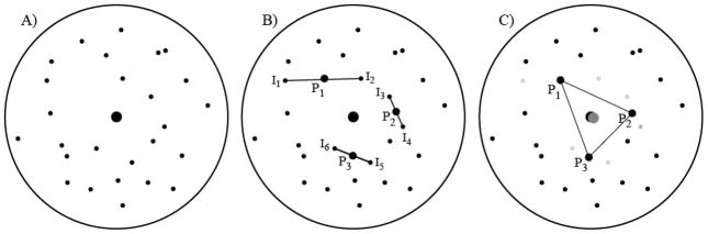
A geometric representation of how parceling works. Each circle represents the domain of possible indicators of a construct. The construct’s ‘true’ centroid is the larger dot in the center of each circle. The average of any two variables is the mid-point of a straight line as depicted in B (the average of three or more indicators would be the geometric center of the area that they encompass). The latent construct that is indicated by the parcels is the center dot in gray that nearly overlaps the true centroid as in C. Figure copyright, Todd D. Little.

Figure 2.

Population measurement model for 6 indicators of a construct (T₁). Tables 1 and 2 show the covariance algebra by which the different sources of variance identified in this graphic display combine.

Moving to Panel B, we have selected six possible indicators. The figure depicts an assignment of indicator 1 (I₁) and indicator 2 (I₂) to parcel 1 (P₁)_, indicators 3 and 4 (I₃ and I₄) to parcel 2 (P₂), and indicators 5 and 6 (I₅ and I₆) are assigned to parcel 3. As mentioned, indicators that are closer to the centroid will have smaller specific variances (the potentially problematic source of variance) than will indicators that are further away. Similarly, any items that are closer to each other will have higher correlations with each other (due to shared specific variances) than they will with other items that are further away. Given these simple geometric properties, we can see that I₂ and I₃ would be more highly correlated with each other than they would be correlated with the actual construct they are supposed to measure. In fact, a CFA model run on the item-level data would have better fit if the residual variances of items I₂ and I₃ were allowed to covary. In addition, because I₁ is quite far away from the centroid of the construct, it contains a high degree of reliable variance related to another construct (i.e., a high specific variance). If that construct were also under investigation, item I₁ may have a secondary loading on that construct.

By taking the average of the indicators that were assigned to each parcel, a new parcel-level indicator is created.² Because these items are all at the same level of communality (and we assume their variances are equal), the parcel-level indicator will be located, geometrically speaking, at the mid-point of the line connecting the two indicators (we assume equal variances for simplicity -- if one item has a larger variance than the other, the parcel-level indicator would be located closer to the item with the larger variance). More specifically, the locations of the larger dots labeled P₁, P₂, and P₃ in Panel B are the locations of the parcel-level indicators that would result from averaging the corresponding item-level indicators. In the C panel of Figure 1, we have connected the three parcels with lines to depict the triangulation on the centroid that the three parcels would now measure. Here, the geometric mid-point of the triangle created by the three parcels is the estimated factor centroid, which, as can be seen, is close to the true centroid. Keep in mind that, when properly modeled, item-level analyses and parcel-level analyses generally should converge on the same centroid and on average they do (see Little et al. 1999).

Test Theory and Measurement Foundations of Parcels

At the heart of building parcels is the basic logic of test theory (MacDonald, 1999). In its hybrid form, classical test theory describes the response to a given variable (x) as comprising three uncorrelated effects:

$$\mathrm{x}=t+s+e$$ (1)

Where x is a variable, t is the true score (whatever the item x is being used to measure), s is the sum of other item-specific effects that contribute to x, and e is purely random noise (i.e., the unreliable measurement error). When variables are indicators of the same construct, the t is shared among all indicators, while s and e are specific to each indicator. For example, if the item, “I have trouble sleeping” is used as an indicator of depression, its true score variance is that which is due to depression, its specific variance is that which is related to aspects of other constructs that are independent of depression such as anxiety, mental illness, sleep disorders, hypochondria, and various response biases. The sum of the variances of t and s is the reliable variance of a given item and the variance of t reflects the communality that an item has with the construct it indicates. In this framework, it is the unique term s that can lead to problematic representations.

For all indicators of all constructs, the s for each indicator is assumed to be uncorrelated with every other s and with the t’s of all other constructs. From the standard assumptions of the classical test theory framework, s and e are normally distributed in the population with a mean of zero and e is orthogonal to both t and s. These assumptions can be violated. The assumption that the each item’s s will be uncorrelated in a given model, for example, is often violated when item-level information is analyzed (e.g., several items that measure depression may also be indicators of anxiety and, as a result, their specific variances would correlate). The sum of s + e for a given item is referred to as its uniqueness; for most applications of SEM this uniqueness is simply the residual variance after accounting for the construct-related true scores in a set of indicators for a given construct. When the assumption of orthogonality among the set of unique factors is violated, a residual covariance among indicators may be needed to accurately represent the measurement structure of the items and the true relations among the constructs.

Indicators of a given construct can vary along a number of related dimensions: scale type, dimensionality, operational specificity, and purity. These four dimensions have overlapping consequences for measurement efficiency and creating parcel-level indicators of constructs in the SEM framework.

Scale type

The strictest scale-type assumption about a set of indicators is that they are parallel in the population. Parallel indicators have equal amounts of true-score variance and equal amounts of unique variance. That is, each item is comprised of the same amount of t, and the variance of (s + e) is the same for all items. The resulting CFA measurement model is one where all items have equal loadings, equal residual variances, and equal intercepts. Essentially parallel indicators are those that have equal loadings and residual variances, but different intercepts. The assumption of parallelism occasionally applies to ability test items (e.g., the simple addition items 4 + 7 and 3 + 8 likely conform to these assumptions), but outside of the ability test realm, the assumption of parallelism is unrealistic for most psychological items.

The next level of scale type, tau-equivalence, is less restrictive but still unrealistic for many constructs outside the ability domain. Tau-equivalent indicators have equal amounts of true score (i.e., all items have equal communality), but the contribution of unique components (i.e., the variance of s + e) varies across items. For example, a set of items measuring positive affect (e.g., “I feel great,” “I feel happy,” “I feel energetic”) could have the same loading on a construct, but their specific components vary because of the specific mood adjective chosen to measure positive affect (i.e., “happy” vs. “energetic”). The resulting CFA measurement model is one where all items have equal loadings but unequal residual variances. Essentially tau-equivalent indicators have equal loadings but unequal intercepts and unique variances.

Finally, the least restrictive assumption (and the assumption necessary to identify a latent construct) is that indicators are congeneric. Congeneric indicators share true-score variance, but the amount of true-score (t) that each indicator contains can be different. In addition, their unique variances differ. For example, on a loneliness scale, the marker item (i.e., “I feel lonely”) would contain more loneliness-related variance than an ancillary item (e.g., “I think others don’t like me”). In the resulting measurement model, loadings and residual variances would vary but intercepts might remain equal. If the intercepts differ, the indictors are essentially congeneric (see Little, Slegers, & Card, 2006, for detailed statistical definitions).

Dimensionality

In terms of dimensionality, items can vary from unidimensional to multidimensional. Unidimensional items are those that only measure a single construct (each item has a single true score source). For example, math test items such as, 7 + 4 and 8 + 3 are unidimensional indicators of the construct, arithmetic skill. Math problems presented in the form of a sentence such as, “Mijke has four bananas, and Alex has seven apples; how many fruit do they have in total?” are multidimensional, because each item assesses several dimensions, including math skill and verbal skill (e.g., x = (t_m + t_v) + s + e, where t_m is math skill, and t_v is verbal skill). When all indicators of a construct have the same multidimensional structure, the shared sources of variance among the items will be inseparable and the shared variance among these items will reflect a multidimensional construct (i.e., a construct that includes several sub-facets and their specific variances, e.g., math skill and verbal skill). On the other hand, when a set of indicators includes items with different multidimensional properties (e.g., an intelligence test composed of numerical facility items, verbal ability items, and spatial reasoning items), the shared variance among all items will reflect a unidimensional construct (e.g., the shared intellective functioning needed to solve all the items, but none of the specific variance associated with math, verbal, or spatial ability). Below, we show how items that share facets can be parceled to create either unidimensional or multidimensional construct representations.

Purity

Finally, items can also vary in the degree to which they are pristine or dirty. Pristine items are often prototypical items for a given construct with a very low amount of specific variance. Such items typically have very clear operational characteristics (e.g., “I am satisfied with my life” is a pristine indicator of the construct life satisfaction). In such cases, the item-specific variance will be negligible relative to the true-score variance of the indicator. Impure (dirty) items contain an extraneous source of variance. For example, “When I think about it, I am happy with my life” is a noisy indicator of Life Satisfaction, because it contains the subordinate clause “When I think about it”. Here, x= t + s_w + s_h + e, where t is the true life satisfaction score, s_w is the specific effect related to the “when I think about it” clause, s_h is the specific component related to the clause “I am happy with my life”, and e is random error.

Noisy items can be thought of as multidimensional but where one of the dimensions is an unintentional or inadvertent source of variance. When two or more noisy items share the same extraneous source of variance, they have correlated specific variances. For example if two items from the hypothetical life-satisfaction scale use the “when I think about it” clause, the s_w would be shared between these two items. Impurity is not typically a characteristic of all indicators; in general, different items have different sources of impurity, so these sources do not become part of the construct representation. Impure items typically give rise to correlated residuals but can also lead to dual loadings (e.g., if a “self-reflection” construct is in the model, the life satisfaction items that have “when I think about it” as a clause may load on the self-reflection construct).

Operational Specificity

Little et al. (2002) described operational specificity in terms of the variability in item content that is allowed by the operational definition of a construct. A construct that is defined narrowly has high operational specificity and leads to a selection of indicators that are highly similar, whereas a construct that is vaguely defined has low operational specificity and allows a much more diverse selection of indicators. For example, a scale that measures the construct, “simple addition skill” is confined to the basic simple addition combinations that are possible. In this case, the items that can be used to indicate the construct of addition skill are highly circumscribed, and both the magnitude of and the variability in the specific variances is very minimal. Constructs such as self-efficacy, depression, and self-regulation, on the other hand, are less precise in their operational definitions. As a consequence, items that can be used to represent such constructs can be quite variable in their make-up. In such cases the specific variance component of each indicator can be quite large and the potential for a dual loading or a correlated residual becomes greater as operational specificity becomes more vague (high diversity indicators; Little et al., 1999).

Although these characteristics of items for certain constructs are overlapping, they are not the same. These characteristics overlap in the sense that they each describe the sources of variance that are present in an item. For example, both unidimensional items and multidimensional items can vary in their purity, they can vary in their operational specificity, and they can vary in terms of scaling (e.g., parallel, tau-equivalent, congeneric).

The Covariance Algebra of Parcels: Reduction of Nuisance Parameters

To understand and appreciate the mathematics underlying why parcels function the way they do, we present some basic covariance algebra formulae. The full derivations and proofs of these formulae can be found in Gibson (2012). Here, we highlight the generalized conclusions gained from studying the sources of variance of a given parcel as compared to the variance of the original indicators. By analyzing the variance of parcels, we can garner a deeper understanding of what happens to the variance when items are averaged to create a parcel. Since SEM is intended as a technique to analyze shared variance among the indicators of latent constructs, analyzing parcel variances clarifies how parceling will affect the models, the parameters of interest and, perhaps, model fit and estimation efficiency.

As we will show, parceling creates a new model that has reduced sampling variability and smaller nuisance parameters. Specifically, parceling reduces the magnitude of specific variances that lead to correlated residuals and dual factor loadings in a given model. When these effects emerge due to sampling variability, parcels minimize their impact by reducing the magnitudes of these sources of variance. Similarly, correlated s variances among items can result in correlated residuals and cross-loadings that exist in the population. Nonetheless, these effects may not be of interest, in which case, a model that minimizes these effects may be preferable. As we will see in this section, parcels not only have reduced unreliable (e) variance, but they also have reduced reliable specific (s) variance. Population effects in the item-level model may be made smaller in the parcel-level model; Nasser & Takahashi, 2003).

When a cross-loading or residual correlation exists in the population, omitting the parameter from the model (i.e., fixing its value to zero) may result in biased structural estimates if the population value is large. If the magnitude of the effect is reduced in the parcel model, it may become a trivial and ignorable effect. In other words, there is a true model in the population for item-level data that has a “true” correlated residual or dual loading that might not get estimated if the disturbance is mistakenly attributed to sampling variability. The impact of such potential errors can be minimized with parceling. That is, a true model also exists in the population for the parcel-level data, but this model is less likely to have meaningfully sized correlated residuals and dual-factor loadings than the item-level solution. These sources of variance are reduced and can become effectively non-influential when they are reduced to a trivial magnitude. We note, however, that it is critical to be sufficiently familiar with the items and to examine item-level solutions before using parcels to diminish the size of nuisance effects. A nuisance effect that is large enough to introduce bias into a model when it is not estimated may seem to disappear in a parceled solution, but the bias may remain (Bandalos, 2008).

When parcels are formed (either by averaging or summing items), whatever variance is shared between items (true score variance) is preserved, while unshared variance (uniquenesses) shrinks. To illustrate the algebra involved, Figure 2 depicts a hypothetical construct (T₁) with six items as indicators. Items 4 and 5 have a correlated residual (due to a shared influence of x). Item 1 has a dual loading on a factor T₃, which is uncorrelated with T₁. Item 6 has a dual loading on factor T₂, which is correlated with T₁. Each item is composed of one part true score stemming from the factor T₁, plus one part specific variance (s₁ to s₆), and one part random error (e₁ to e₆). In addition, items with a correlated residual add one part of the source of shared variance (x) and items with a dual loading add one part of the source of the dual loading (T₂ or T₃). For the sake of keeping the algebra simple, we assume that all factor loadings are equal to 1 in the population (that is, every item is composed of the same amount of T₁; items are tau-equivalent). The correlation between T₁ and T₂ is illustrated using C, which is their common source of variance. In addition, T₁ is influenced by U₁ (the unique variance of construct T₁) and T₂ is influenced by U₂ (the unique variance of construct T₂). U₁, U₂, and C are independent sources of variance. In our examples, we focus on three-item parcels but the equations can be generalized to any number of items.

Assigning items with a correlated residual to different parcels

The first column of Table 1 considers the “simple parcel” constructed of items 2, 3, and 4, and explains the variance components of this parcel. First, the parcel is expanded into all the components that make up each item. Because a variable’s variance is simply its covariance with itself, the parcel variance can be expanded into the covariance of each term in the sum with every other term. Most of these terms reduce to zero because, by definition, each source of variance is unique (e.g., the random error of one item does not covary with that of any other item, or with any specific variance, or with the true score). The terms that do not reduce to zero can be restated as variances. Because the true score T₁ is part of each of the three items, its variance is represented nine times more than each other variance component (this is due to the rule var(aX) = a² var(X), where a is a constant). The resulting parcel’s variance is composed of one part var(T₁), and 1/9^th of a part of every other source of variance, including var(x), the variance shared with item 5. As this example shows, if two items that share a correlated residual are placed into two different three-item parcels, the magnitude of the residual covariance between those two parcels will be reduced to be 1/9^th of what it was prior to parceling.

Table 1.

Brief Derivations of the Variance of One or Both Items with a Correlated Residual

	Single Item with Correlated Residual	Both Items with Correlated Residuals
Indicators	I2 = T1 + s2 + e2 I3 = T1 + s3 + e3 I4 = T1 + s4 + x + e4	I3 = T1 + s3 + e3 I4 = T1 + x + s4 + e4 I5 = T1 + x + s5 + e5
Parcel	$\frac{1}{3}\left[I_2+I_3+I_4\right]$	$\frac{1}{3}\left[I_3+I_4+I_5\right]$
Variance of the parcel	$var\left(\frac{1}{3}\left[3T_1+s_2+s_3+s_4+x+e_2+e_3+e_4\right]\right)$	$var\left(\frac{1}{3}\left[3T_1+2x+s_3+s_4+s_5+e_3+e_4+e_5\right]\right)$
Restated as a covariance	$\frac{1}{9}cov\left(\begin{array}{l}3T_1+s_2+s_3+s_4+x+e_2+e_3+e_4,\hfill \\ 3T_1+s_2+s_3+s_4+x+e_2+e_3+e_4\hfill \end{array}\right)$	$\frac{1}{9}cov\left(\begin{array}{l}3T_1+2x+s_3+s_4+s_5+e_3+e_4+e_5,\hfill \\ 3T_1+2x+s_3+s_4+s_5+e_3+e_4+e_5\hfill \end{array}\right)$
Expanded with zero terms removed	$\frac{1}{9}\left[\begin{array}{l}cov\left(3T_1,3T_1\right)+cov\left(s_2,s_2\right)+cov\left(s_3,s_3\right)\hfill \\ +cov\left(s_4,s_4\right)+cov\left(x,x\right)+cov\left(e_2,e_2\right)\hfill \\ +cov\left(e_3,e_3\right)+cov\left(e_4,e_4\right)\hfill \end{array}\right]$	$\frac{1}{9}\left[\begin{array}{l}cov\left(3T_1,3T_1\right)+cov\left(2x,2x\right)\hfill \\ +cov\left(s_3,s_3\right)+cov\left(s_4,s_4\right)+cov\left(s_5,s_5\right)\hfill \\ +cov\left(e_3,e_3\right)+cov\left(e_4,e_4\right)+cov\left(e_5,e_5\right)\hfill \end{array}\right]$
Restated as variances	$\begin{array}{l}\frac{1}{9}\left[\begin{array}{l}9var\left(T_1\right)+var(s_2)+var\left(s_3\right)+var\left(s_4\right)\hfill \\ +var\left(x\right)+var\left(e_2\right)+var\left(e_3\right)+var\left(e_4\right)\hfill \end{array}\right]\\ var\left(T_1\right)+\frac{1}{9}\left[\begin{array}{l}var\left(s_2\right)+var\left(s_3\right)+var\left(s_4\right)+var(x)\hfill \\ +var\left(e_2\right)+var\left(e_3\right)+var\left(e_4\right)\hfill \end{array}\right]\end{array}$	$\begin{array}{l}\frac{1}{9}\left[\begin{array}{l}9var\left(T_1\right)+4var(x)+var\left(s_3\right)+var\left(s_4\right)\hfill \\ +var\left(s_5\right)+var\left(e_3\right)+var\left(e_4\right)+var\left(e_5\right)\hfill \end{array}\right]\\ var\left(T_1\right)+\frac{4}{9}var(x)+\frac{1}{9}\left[\begin{array}{l}var\left(s_3\right)+var\left(s_4\right)+var\left(s_5\right)\hfill \\ +var\left(e_3\right)+var\left(e_4\right)+var\left(e_5\right)\hfill \end{array}\right]\end{array}$

Note. Figure 2 shows the item-level model that describes these items, and all components of the equations. T₁ is not expanded into C + U₁ here, for simplicity.

If items 2–4 were combined to form Parcel 1, and items 1, 5, and 6 combined to form Parcel 2, the x component that was in items 4 and 5 would still be shared across the two parcels. The magnitude of the shared x variance in each parcel, however, would be reduced to one ninth of its original variance, and the residual covariance between Parcel 1 and Parcel 2 would also be reduced to one ninth of its original size. If the original x component was quite large (e.g., if the standardized residual covariance between items 4 and 5 was .45) then reducing it by one ninth (i.e., to .05) may or may not yield a non-negligible covariance that would still need to be estimated in a parcel-level model. If, on the other hand, the correlated residual at the item level was small, the information in the resulting parcel would be reduced to a trivial level that would not be significant if it were estimated and it would likely not result in any appreciable parameter bias. This simple parcel is one way in which, by combining items to reduce unwanted variances, parceling can create indicators with better measurement properties.

Assigning items with a correlated residual to the same parcel

The second column of Table 1 explains the variance components of the parcel constructed of items 3, 4, and 5. In this parcel, the x variance that items 4 and 5 share is not reduced to the same degree that uncorrelated residuals are reduced. Following the same algebraic steps as the previous example, we can see that, because it is shared among 2 items making up the parcel, var(x) only reduces to 4/9^ths of its item-level variance. The x variance, however, is not shared by any other items or parcels. Because x does not affect any other item or parcel, the x variance will remain as residual variance that is not shared with any other construct or indicator in the model. In this case, the x information is still in the model but because it does not covary with anything else in the model, it can simply be represented as part of the residual variance of the parceled indicator and will not impact model fit or parameter estimates. For this reason, when a correlated residual is evident in an item-level solution, the most advantageous parcel solution may be one that aggregates those correlated items together (“shared uniqueness” vs. “distributed uniqueness”; Hall, Snell, & Foust, 1999).

Assigning items with cross-loadings to a parcel

Table 2 describes the variance components of parcels that contain an item that cross-loads on another factor. The first column considers a parcel formed of items 2, 3, and 6. Item 6 loads on both constructs T₁ and T₂, which are correlated. From Figure 2, T₁ is comprised of equal parts U₁ and C while T₂ is comprised of equal parts U₂ and C. As we saw in previous examples, when only one item in a parcel contains a particular source of variance, that source of variance will be a much smaller proportion of the parcel’s variance than it was of the item’s variance. Parceling item 6 with other items that do not have any tendency to cross-load on T₂ will reduce the size of the cross-loading (compared to the item-level solution), because the U₂ variance is not shared with any other item in the parcel. As Table 2 shows, the parcel will contain only 1/9^th of the U₂ variance that was in Item 6, resulting in a covariance between the parcel and T₂ that is one third of that between Item 6 and T₂. The amount of C variance (the source of the correlation between T₁ and T₂) in the parcel is 16/9ths of what it would be if there were no cross-loading. That is, in addition to having a diminished covariance with the unique part of T₂, the parcel has an elevated covariance with the shared part of T₁ and T₂. If this parcel were used as an indicator of T₁ (with its cross-loading on T₂ constrained to zero), it would likely lead to an upwardly biased estimate of the covariance between T₁ and T₂.

Table 2.

Brief derivations of the variance of two types of parcels with cross-loadings

	Cross-loading with correlated factors	Cross-loading with uncorrelated factors
Indicators	I2 = T1 + s2 + e2 = U1 + C + s2 + e2 I3 = T1 + s3 + e3 = U1 + C + s3 + e3 I6 = T1 + T2 + s6 + e6 = U1 + C + U2 + C + s6 + e6	I1 = T1 + U3 + s1 + e1 = U1 + C + U3 +s1 + e1 I2 = T1 + s2 + e2 = U1 + C + s2 + e2 I3 = T1 + s3 + e3 = U1 + C + s3 + e3
Parcel	$\left(\frac{1}{3}\right)I_2+I_3+I_6$	$\left(\frac{1}{3}\right)I_1+I_2+I_3$
Variance of the parcel	$var\left(\frac{1}{3}\left[3U_1+4C+U_2+s_2+s_3+s_6+e_2+e_3+e_6\right]\right)$	$var\left(\frac{1}{3}\left[3U_1+3C+U_3+s_1+s_2+s_3+e_1+e_2+e_3\right]\right)$
Restated as a covariance	$\frac{1}{9}cov\left(\begin{array}{l}3U_1+4C+U_2+s_2+s_3+s_6+e_2+e_3+e_6,\hfill \\ 3U_1+4C+U_2+s_2+s_3+s_6+e_2+e_3+e_6\hfill \end{array}\right)$	$\frac{1}{9}cov\left(\begin{array}{l}3U_1+3C+U_3+s_1+s_2+s_3+e_1+e_2+e_3,\hfill \\ 3U_1+3C+U_3+s_1+s_2+s_3+e_1+e_2+e_3\hfill \end{array}\right)$
Expanded with zero terms removed	$\frac{1}{9}\left[\begin{array}{l}cov\left(3U_1,3U_1\right)+cov(4C,4C)+cov\left(U_2,U_2\right)\hfill \\ +cov\left(s_2,s_2\right)+cov\left(s_3,s_3\right)+cov\left(s_6,s_6\right)\hfill \\ +cov\left(e_2,e_2\right)+cov\left(e_3,e_3\right)+cov\left(e_6,e_6\right)\hfill \end{array}\right]$	$\frac{1}{9}\left[\begin{array}{l}cov\left(3U_1,3U_1\right)+cov(3C,3C)+cov\left(U_3,U_3\right)\hfill \\ +cov\left(s_1,s_1\right)+cov\left(s_2,s_2\right)+cov\left(s_3,s_3\right)\hfill \\ +cov\left(e_1,e_1\right)+cov\left(e_2,e_2\right)+cov\left(e_3,e_3\right)\hfill \end{array}\right]$
Restated as variances	$\begin{array}{l}\frac{1}{9}\left[\begin{array}{l}9var\left(U_1\right)+16var(C)+var\left(U_2\right)+var\left(s_2\right)\hfill \\ +var\left(s_3\right)+var\left(s_6\right)+var\left(e_2\right)+var\left(e_3\right)+var\left(e_6\right)\hfill \end{array}\right]\\ var\left(U_1\right)+\frac{16}{9}var(C)\\ +\frac{1}{9}\left[\begin{array}{l}var\left(U_2\right)+var\left(s_2\right)+var\left(s_3\right)+var\left(s_6\right)\hfill \\ +var\left(e_2\right)+var\left(e_3\right)+var\left(e_6\right)\hfill \end{array}\right]\end{array}$	$\begin{array}{l}\frac{1}{9}\left[\begin{array}{l}9var\left(U_1\right)+9var(C)+var\left(U_2\right)+var\left(s_1\right)\hfill \\ +var\left(s_2\right)+var\left(s_3\right)+var\left(e_1\right)+var\left(e_2\right)+var\left(e_3\right)\hfill \end{array}\right]\\ var\left(U_1\right)+var(C)\\ +\frac{1}{9}\left[\begin{array}{l}var\left(U_3\right)+var\left(s_1\right)+var\left(s_2\right)+var\left(s_3\right)\hfill \\ +var\left(e_1\right)+var\left(e_2\right)+var\left(e_3\right)\hfill \end{array}\right]\end{array}$

Note. Figure 2 shows the model that describes these items, and all components of the equations.

The second column of Table 2 depicts a similar situation involving a cross-loading on an uncorrelated factor (T₃), by considering the parcel made up of items 1–3, where item 1 contains variance from both T₁ and T₃. T₃ is composed only of unique variance (U₃), so it is uncorrelated with T₁. Here, the parcel again contains1/9^th of the U₃ variance that was in the original item, but it contains no additional C variance. Using this parcel as an indicator of T1 (with its cross-loading on T₂ constrained to zero) would be less problematic. In general, the algebra suggests that item cross-loadings might be “parceled out” more effectively (that is, with less potential for biasing the structural model) when the two factors on which the items load are not highly correlated or when the cross loading is due the unique variance to the 2^nd construct and is unrelated to the common variance between the two constructs.

In summary, putting items together that share a correlated residual will either reduce the magnitude of the correlation (when the two items are allocated to different parcels) or relegate the information to be contained in the indicator’s uniqueness (when the two items are allocated to the same parcel). If the specific factor information is shared across two parcels, the magnitude of the correlation will be reduced to a fraction of its original magnitude, depending on the number of items that are used to create the parcels. Cross-loadings on uncorrelated factors are diminished in the same way, though cross-loadings on correlated factors may produce bias in the structural model. In each of the scenarios outlined in Tables 1 and 2, the key question becomes whether the reduction in magnitude is sufficient to ignore the source of the nuisance variance, and if ignored, whether the remaining information would have a meaningful influence on the structural parameters of a model. In sample data, this question may be addressed by examining and comparing the item-level and the parcel-level models. Future simulation work should address these questions more generally.

Sources of error

One key assumption of a statistical model being fit to the sample is that it is the correct model for the data (e.g., a cross loading is truly a cross loading and not a result of sampling error). In other words, we assume that the model is true in the population. Of course, we, as mere mortals, never know what exactly things are like in the population. As McCallum and Austin (2000; see also Box, 1979) point out, however, “…all models are wrong to some degree, even in the population, and the best one can hope for is to identify a parsimonious, substantively meaningful model that fits observed data adequately well” (p. 218). Across different samples, some variability in model fit and parameter estimates will result inevitably from the fact that a model is going to be wrong to some degree anyway.

These sources of error are reflected in the specific variances of the indicators, which are not likely to have exactly zero correlations with other sources of error or exactly zero-valued loadings on other constructs in the model. These kinds of population-level errors are referred to as parsimony error, which is different from misspecification error (Cheung & Rensvold, 2001). With misspecification error, a neglected parameter is non-trivial in the population and ignoring it will lead to biased parameters, whereas parsimony error is the aggregate impact of the trivial non-zero values that occur in the population. Parsimony error primarily impacts model fit and can be subject to sampling error.

The different sources of error that can arise add layers of complexity. Sampling error is the inherent variability around the true population values for a given parameter estimate of any statistical model based on a finite sample. Sampling variability is conceptualized by drawing repeated finite samples (of a given size) from the population. On average, a given random sample will provide estimates of the population parameters that are equal to the true population values, but there will be variability in these estimates from sample to sample. That is, any given sample may deviate from the population values to some degree. The larger the sample size, the lower the sampling variability. Sampling error is not just a concept related to samples of individuals from a population, but it can also pertain to sampling items from a population of items. The more homogenous the population of items is the lower is the item-sampling variability. This later idea is captured by the concept of selection diversity that was introduced by Little et al. (1999) in their simulation of indicator selection (see also Little et al., 2002). When selection diversity is low, item-sampling variability is also low, bias is minimal, and efficiency is high (Little et al., 1999).

Summary of the Pro- and Anti-Parcel Arguments

The pro- and anti-parcel arguments that persist generally are centered on situations in which items are weak, variable, and/or noisy (e.g., contain dual loadings, correlated residuals) in their representation of an underlying construct and when the construct is multidimensional in nature. To understand the original fodder of the debate, we highlight some of the arguments both pro and con (for a more thorough review see Little et al., 2002; see also Matsunaga, 2008).

One argument against using parcels is that constructs are frequently multidimensional, and indicators of multidimensional constructs typically have multiple sources of variance (Marsh, 1998). When these multiple sources of variance combine into a common construct, the interpretation of what constitutes the construct can be muddied. The nature of a multidimensional construct also muddies the ability to identify which constituent of the multidimensional construct is involved when the construct is placed into the context of a multiple-construct SEM model. For example, if the dimensions of the construct have different relations with other constructs in the model, these differences will not appear. As researchers have pointed out (see parceling methods, below), when parcels are created using inappropriate techniques, a multidimensional construct will not be represented clearly or cleanly. An inappropriate parceling scheme can make a multidimensional construct look like it is unidimensional, obscuring the multifaceted relations it has with other parts of the model (Bandalos, 2002; Bandalos & Finney, 2007).

The corresponding pro-parcel argument is that, when properly constructed, parcels can clarify representations of even multidimensional constructs (Graham, Tatterson, & Widaman, 2000; Graham, 2004; Hall et al., 1999). Below, we review some suggestions on how to form parcels of indicators of a multidimensional construct that preserves the common construct variance while minimizing unrelated specific variance.

A second main argument against using parcels is that they may mask model misspecifications. That is, true misspecifications that stem from item properties (e.g., cross-loadings or residual correlations) may be difficult to detect when those items are folded into a parcel. Such misspecifications can lead to biased estimates of other model parameters (e.g., structural parameters; Bandalos & Finney, 2007; Hall et al., 1999; Kim & Hagtvet, 2003; Landis, Beal, & Tesluk, 2001; Little et al., 2002; Matsunaga, 2008; Meade & Kroustalis, 2006; Rogers & Schmitt, 2004; Sass & Smith, 2006). For example, several studies have found that, though model fit indices almost always improve with parceling, structural parameters may not become less biased (Landis et al., 2001; Rogers & Schmitt, 2004). The good model fit with parceling may lead to a false sense that a misspecification is not present and the reported findings would be biased. More specifically, as shown in the algebra proofs (see Tables 1 and 2), when items have a dual loading or a correlated residual as part of their structure, the source of nuisance variance is not totally eliminated even when the item is placed in a parcel with other items that do not have a dual loading or a correlated residual. When parcels are used in this context, model fit can suggest a sound representation of the data even though the model is not properly specified (Hall et al, 1999; Rogers & Schmitt, 2004).

The corresponding pro-parcel view on the issue of misspecification rests on two ideas. First, when items are parceled, the rate of Type II errors will be reduced (e.g., researchers will not conclude that a cross-loading exists in the population when they really do not). Second, careful and well-informed modelers are able to identify notable misspecifications that may have an impact on structural parameter estimates because they are keenly aware of the item-level relations. These arguments assume that potential misspecifications are detectable when they arise from true population misfit, and that researchers will not confuse true misspecification and model misfit with a sampling perturbation and parsimony error. Careful modelers are familiar with item contents prior to parceling and they know where to look to see if a correlated residual or dual loading remains of a magnitude that should be estimated³.

When a modification to the measurement model (e.g., adding a correlated residual or cross-loading) is warranted, the reason for adding this parameter to the model must be theoretically justified. Inexplicable model changes should be discouraged as they are likely emanate from the variability of the sample. On the other hand, a reasoned adjustment based on a knowledgeable understanding of the indicator under scrutiny is likely to reveal that an indicator has a valid and theoretically meaningful sub-facet that relates to another indicator or another factor. This relation is expected to replicate in future work with the same set of indicators. From this perspective, the potential for misspecification errors that computer simulations highlight can be mitigated by the intelligent human factor and item-level awareness. Skilled modelers, for example, routinely examine the fitted and standardized residuals, model modification indices, and other indictors of local misfit (e.g., inflated standard errors for some parameters compared to others). Such modelers know that well-fitting models are not necessarily good models, nor are they necessarily accurate approximations of the underlying data (i.e., many roughly equivalent models can show the same good model fit and yet not represent the processes underlying the observed data). By fitting a supplemental item-level model, many of the item quirks (specific variances, cross-loadings that are conceptually meaningful) will become obvious, and can be taken into account when making a decision of which items to parcel.

In ideal situations, researchers are both practiced modelers and highly familiar with and confident in their items. This familiarity, however, varies across research areas because research areas vary in their degree of maturity. A mature research area is typified by well-developed and psychometrically sound measures. The magnitudes of association among the focal constructs in the area are replicable and refined. Less mature research areas are muddled in the mire that characterizes the discovery of new relations. Parcels, as vehicles for bringing the manifest information into the latent space, are useful in either realm. In mature research areas, enough information exists to inform precise parcel allocation plans that have the greatest empirical and theoretical support. In less mature research areas, on the other hand, more exploration of the item-level relations may be needed to inform the parcel building steps.

In addition to the counter-arguments given above, those who argue for the usefulness of parcels point out that they can have a number of statistical and analytical advantages over item-level analyses (Little et al., 2002 & Matsunaga, 2008, for reviews; see also Bandalos & Finney, 2007). These advantages can be summarized into two classes, their fundamental psychometric characteristics and their behavior when estimating a model. These advantages are summarized in Table 3. As detailed in Little et al. (2002), the psychometric principles that support the empirical benefits outlined in Table 3 are based on the Principle of Aggregation and the Law of Large Numbers. The Principle of Aggregation (e.g., Rushton, Brainerd, & Pressley, 1983; Matsunaga, 2008; Nunnally, 1978) is a selection-based idea stating that any one item is less representative of a construct than the average of many items from the same pool of potential indicators of that construct. The Law of Large Numbers is a sampling-based idea suggesting that more samples of items from a given domain of items will yield a more precise set of parameter estimates (less sampling variability; Little et al., 2002; Matsunaga, 2008) and the increased number of items to represent a construct will have a normalizing tendency on the distribution of scores (Bandalos, 2002; Hau & Marsh, 2004; MacCallum, Widaman, Zhang, & Hong, 1999; Matsunaga, 2008, Nunnally, 1978), which slakes the thirst of the ML estimator (Yuan & Schuster, in press). Many of the advantages listed in Table 3 are direct consequences of the covariance algebra reviewed above.

Table 3.

Key advantages of parcels vs. items

Psychometric Characteristics Parcels (as opposed to the items) have… Higher reliability Greater communality Higher ratio of common-to-unique factor variance Lower likelihood of distributional violations More, tighter, and more-equal intervals

Model Estimation and Fit Characteristics Models with parcels (as opposed to the items) have… Fewer parameter estimates Lower indicator-to-sample size ratio Lower likelihood of correlated residuals & dual factor loadings Reduced sources of sampling error

Note. These advantages pertain to the smaller set of parcels that are made up from a larger set of items. The advantages accrue based on the principle of aggregation and the law of large numbers.

The first three psychometric advantages that are listed in Table 3 (higher reliability, greater communality, higher ratio of common-to-unique factor variance) are saying essentially the same thing. Based on the Principle of Aggregation, each parcel will have greater reliability than any individual item that is used to create the parcel. As a result of having greater reliability, a given parcel will have a larger proportion of true-score variance to unique variance than any item used to build it (except in rare cases when individual item reliability is extremely low; Yuan, Bentler, & Kano, 1997). The indicator-level reliability will also make the factor loadings stronger (increased communality) and the residual variances smaller. As a result, the ratio of common-to-unique factor variance is higher. All three of these related features of parcels are beneficial to improving the psychometric properties of the data that are fit in an SEM model.

Another beneficial psychometric characteristic of parcels as opposed to items is the lower likelihood of distributional violations. That is, aggregating items that may be non-normal into a parcel generally will lead to a more normal indicator than any of the individual items (Bandalos, 2008; Nasser & Takahashi, 2003; cf.; Alhija & Wisenbaker, 2006; Hau & Marsh, 2004). This normalizing tendency of aggregating items into parcels is graphically depicted in Matsunaga (2008; see also Rushton et al., 1983; Nunnally, 1978). Similarly, aggregating categorical items produces a new indicator that will be more continuous than the individual items. Models based on ordinal items with few categories are typically estimated with limited-information categorical estimators (e.g., diagonally weighted least squares, the default in Mplus), which are less efficient than ML (Yang, Nay, & Hoyle, 2010). Parcels can often satisfy the minimal needs of the ML estimator (Yuan & Schuster, in press).

The other advantages listed in Table 3 focus on model estimation benefits. The reduced sampling error and likelihood of correlated residuals and dual loadings has already been highlighted above. The other benefits of lowering the indicator-to- sample ratio and reducing the number of parameter estimates are rather obvious advantages. For small models the reduction in parameter estimates may not seem like much of a benefit, but when larger models are involved (see an example below), using parcels can improve model convergence and model stability. Of course, the model fit measures also show improvements, but this global model fit improvement must be interpreted in the context of evaluating the residuals and modification indices. As we have mentioned, improved model fit does not always imply a truer model (Bandalos, 2008).

Many researchers have pointed out that parcels are almost always a better choice than scale scores (i.e., total aggregation; Coffman & MacCallum, 2005; MacCallum & Austin, 2000). Even when scales are adjusted for unreliability, reliable specific variance cannot be removed from a scale, resulting in biased models (Coffman & MacCallum, 2005). When a single scale composed of many items is used to measure a construct, it is still very common practice to use path analysis models based on the total scale score, rather than using an item-level or parcel-level latent variable model (MacCallum & Austin, 2000).

When applied to multiple group and/or longitudinal settings, the particular parceling scheme that is employed must be the same for each group and each time of measurement. If different item-to-parcel allocations are made across groups or times of measurement, there is no way to legitimately evaluate the factorial invariance of the constructs. In this regard, parcels also have potential advantages in the context of invariance testing. Because the unique variances of items are minimized and the ratio of true-score variance to error variance is improved, testing for measurement invariance at the parcel level of aggregation can be justifiable. Even if a prior item-level analysis revealed some evidence of differential item functioning (DIF) or lack of measurement invariance across two or more groups (or time points), the aggregation of two or more variables may show no evidence of DIF or lack of invariance (Meade & Kroustalis, 2006).

Given that evidence of DIF/noninvariance is fundamentally a problem related to the specific variance of an item, parcels provide a means to potentially trivialize the offending specific variance of an item by reducing the magnitude of its impact in a given analysis. If the parcel-level aggregate no longer shows a significant difference across groups or across time, then invariance at the higher level of aggregation is supported by the data (Bagozzi & Edwards, 1998; see also Nesselroade, Gerstorf, Hardy, & Ram, 2007). The new parcel-level indicator, with the aggregate of true-score variance and the reduction of the specific variances becomes the level at which measurement invariance holds. Researchers would, of course, not be justified in concluding that the individual items are invariant across groups or across time. Parceling cannot allow researchers to detect noninvariance/DIF in individual items, only an item-level analysis can accomplish that goal. Here, a given parcel scheme would be a strong statement of theory and the particular items that are designated to be combined would be expected to show the same effect when parceled together in repeated samples of the same context, samples from new contexts, as well as in samples of younger or older participants. If the intent is to test measurement invariance using a parceling scheme, parcels should be chosen based on theory: each parcel should be a theoretically meaningful set of items (as opposed to a random selection of items), where testing its invariance across groups is meaningful.

Understanding the structure of the data and the items is not the same goal as understanding the nature of the construct. If the former is the goal (i.e., to understand how the items are related to the constructs they purport to measure, whether DIF is evident, and how the items may relate to constructs) then clearly parcels would not be used. If the goal is to understand the construct and its relation to other constructs of interest, then well-applied parceling can be used to minimize the specific variances of each item (which are not of interest) and to make the measurement model a parsimonious representation of the construct. We would argue that most dual loadings or correlated residuals lead to a better understanding of items, which are contaminated by many sources of variance. This information is certainly important, but once the researcher progresses past the point of studying the items and is interested in the latent structure, these correlated residuals and cross-loadings become nuisance parameters that compromise the parsimony of the model.

Parceling Strategies

Parceling, as a measurement technique, is based on the statistical principles discussed above. Thoughtful and knowledgeable understanding of the items and the data are critical to the effective use of parcels. In other words, knowing the items and their theoretical content as well as the behavior of the items in a given sample (e.g., running an item-level EFA to examine the item-level content, reviewing the matrix of correlations, and running an item-level reliability analysis) are critical first steps in parcel creation when the goals of a study are to examine the relations among constructs. This step is too often skipped (Williams & O’Boyle, 2000). Similarly, Hagtvet and Nasser (2004; Kim & Hagtvet, 2003) have suggested beginning with a “two-facet” model, where to-be-parceled items are modeled as indicators of latent sub-factors of the construct of interest. Like running an item-level EFA or CFA, this procedure allows researchers to examine the relations among items (including correlated residuals) before settling on a parceling solution.

There are times, as mentioned, when the use of item parcels is not warranted, such as when the empirical question is about the behavior of the items during scale development. In addition, we have described various reasons why creating parcels to use as indicators of latent constructs can be justifiable. On the other hand, there may also be times when the set of items to be analyzed are all well behaved (e.g., normally distributed, continuous, pristine, and unidimensional with little sampling error). In such circumstances, a given set of models may easily address and answer one’s theoretical questions and the use of items or parcels would become a matter of taste.

From a practical viewpoint, however, researchers are including more constructs in their tested SEM models. A simple five construct model, for example, would have 80 degrees of freedom and 40 parameter estimates if one used 3 parcels per construct. A two time point version of such a model would involve more complexity, especially when the residuals of individual indicators are allowed to correlate over time, but the resulting model would still be tractable in terms of the number of parameters and the quality of the solution. In contrast, this same model is fit to the item-level indicators, supposing 9 items per construct, the model would have 3825 degrees of freedom and at least 270 parameter estimates (assuming no correlated residuals or dual loadings resulting from the item-level analysis). Such models become almost intractable to estimate at the item level even in immense samples.

Little (in press) has argued that each construct of an SEM model should be defined by a just-identified measurement space – that is, three indicators per construct. Such models provide superior tests of structural model parameters because the constructs are defined precisely. With four or more indicators per construct, each construct has degrees of freedom generated from the measurement model for each construct as well as the between-construct relationships. Evaluating model fit is thereby confounded by there being two sources of model fit. With just two parceled indicators per construct, locally underidentified measurement spaces can result in high rates of nonconvergence and improper solutions (Nasser & Wisenbaker, 2003; unless equality constraints on the loadings are imposed; Little et al., 1999). Thoughtful parceling can produce a just-identified measurement structure that represents the whole set of items. In doing this, transparency and ethical behavior are important. Researchers need to be clear and honest about their parcel-selection process, and their reasons for using parcels as opposed to items. Under no circumstances is it justifiable to try multiple parcel allocation schemes until one arises that results in the best outcome (e.g., good model fit, or significant structural paths). For these reasons, it is especially important to select an appropriate parcel allocation scheme a priori according to some tested method (we review many of these methods next).

Univariate approaches

Univariate parceling approaches are those that only consider the set of indicators of a single construct at a time when constructing parcels. The most basic parceling approach in this context is random parceling, where items are randomly assigned to parcels. Bandalos and Finney (2001) found that researchers most frequently employ some method of random assignment of items when using parcels in their research, although more recent surveys suggest that other methods are gaining in popularity (Williams & O’Boyle, 2008). Unfortunately, random parceling is predicated on the strong assumption that, in the population, all items are interchangeable. For this reason, it is rarely appropriate, though many authors have advocated random parceling with unidimensional indicators (e.g., Matsunaga, 2008; Sass & Smith, 2006; Landis, Beal, & Tesluk, 2001; Yang, Nay, & Hoyle, 2010; Yuan, Bentler, & Kano, 1997). When one has a large set of items from which to draw in creating parcels and when the items have reasonably good communality (i.e., high loadings in an item-level measurement model), random allocation may be warranted. For instance, parcels of voxels for a region of interest from an fMRI study would offer enough items (voxels) to allow a random assignment process in building parcels. In other words, random parceling can be a good strategy when sampling error is low (large N, many items, high item communality, low item diversity; see Sterba & MacCallum, 2010). In the majority of models, however, these conditions are not met. Even when items are unidimensional indicators of straightforward constructs and there are no cross-loadings or correlated residuals, variability in structural model parameter estimates from one parcel allocation to the next occurs when items have high amounts of sampling error (Sterba & McCallum, 2010). This variability can result in very different conclusions depending on how the random draw came out.

A strong impetus to use parcels often arises when ideal conditions are not met, such as when N is small. With small N, the extra benefit of more reliable items and fewer parameters to estimate can make the difference between a model converging or not. Ledgerwood and Shrout (2011) showed that, with small N, latent variable models can have lower power to detect structural parameters than path models based on scale scores. One way they suggested to increase the power of latent variable models is to create parcels instead of items, and constrain the parcel loadings to equality (of course, this is only appropriate when the parcels have similar measurement properties -- essentially tau equivalent or parallel in nature). Williams and O’Boyle (2008) reported that the most commonly reported reason for using parcels was to improve the sample size to model size ratio. If random assignment is the method of choice, Sterba and MacCallum (2010) suggested using a procedure that takes the average model results over hundreds or thousands of item-to-parcel allocations. Code for doing this (using SAS followed by Mplus) is available at www.vanderbilt.edu/peabody/sterba/parcel/index.htm, or an R function is available in the package semTools (Pornprasertmanit, Miller, & Schoemann, 2012). This method has the added benefit of providing an estimate of the amount of parcel-allocation variability for a particular set of items. Alternatively, there are several purposeful univariate parceling methods that aim to take advantage of the differences among items (e.g., differing communalities, different sources of residual variance, cross-loadings, etc.) and may therefore be more flexible and more appropriate than random parceling.

Most measurement tools in the social and behavioral sciences have gone through a careful development and validation process. Published information on item characteristics from a large norming sample, or from a large body of previous studies may be available. In these situations, ample information exists to create parcels that will optimize the representation of the corresponding latent construct(s). As the section on the covariance algebra of parcels outlines, the goal is to maximize the shared true score information and to minimize the reliable specific variances of the indicators (see also Little et al., 2002). If prior empirical information about the items is readily available, then a defensible plan for parcel building should easily emerge. For example, if two items are known to have correlated residual variance, they should probably be placed in the same parcel, and if two items are known to have cross-loadings with another construct, they could be placed together into a parcel that is allowed to cross-load on that construct. If empirical information about the items is limited, preliminary item-level models are essential to supplement the process of creating an optimal set of parcels for representing the constructs under scrutiny.

The parceling example depicted in Figure 1 is not necessarily the optimal set of parcels that could have been created from the chosen indicators. In practice, we do not know the true location of a construct’s centroid; we can only try to approximate an optimal solution given the items that were selected to represent the construct in the first place. With a balancing approach (see also “single factor analysis” parceling, Landis et al., 2001), the item with the highest item-scale correlation is paired with the item that has the lowest item-scale correlation. The next highest and next lowest items are paired in the second parcel. The third highest and third lowest are paired to form the third parcel. If more items are available, the process continues with the 7^th lowest joining the third parcel, the 8^th lowest joining the second parcel and the 9^th lowest joining the first parcel, etc.). The rationale behind this approach is that an item with a high loading would provide strong support for the construct to match with a weaker item and it attempts to create replicates of the overall factor structure in each of the parcels, creating a set of tau equivalent or parallel parcels (Rogers & Schmitt, 2004; Landis, Beal, & Tesluk, 2000; Sass & Smith, 2006; Yang, Nay, & Hoyle, 2010). Given that the specific variances are reduced, the amount of reduction in the weak item is relatively pronounced. When items are generally unidimensional, this approach performs well but it is not ideal for multidimensional constructs (Rogers & Schmitt, 2004; Landis et al., 2000).

Two parceling strategies that do not assume unidimensional items are correlational parceling (Landis et al., 2001; Rogers & Schmitt, 2004), where the items that correlate most strongly with each other are assigned to a parcel, and facet-representative parceling, where items that share secondary facet-relevant content are chosen to belong to the same parcel (Little et al., 2002; Kim & Hagtvet, 2003; Hagtvet & Nasser, 2009 -- Hall et al., 1999 called this a “shared uniqueness” strategy). Both of these strategies aim to combine items that share reliable specific variance. Both Rogers and Schmitt (2004) and Landis et al. (2001) found that radial or correlational parceling succeeded at maintaining the relation between model fit and parameter bias when parceling multidimensional items. That is, when structural parameters were biased, the model was most likely to display poor fit when these methods were used. In contrast, parceling methods that aimed to create “balanced” parcels (i.e., choosing parcels by alternating high and low correlations or loadings) tended to result in the best-looking model fit (i.e., good fit indices and no modification indices) despite biased structural estimates. Similarly, Hall et al. (1999) found that the shared uniqueness strategy led to less bias in parameter estimates. This result is not unexpected in that all these parceling methods attempt to group items that are highly related to each other together. These groups of similar items are more likely to behave like a facet, and therefore are less likely to obscure the construct structure.

Table 4 shows the variance composition when multidimensional items are combined to form parcels using either the facet representative strategy (Kishton & Widaman, 1994; Little et al., 2002) or the domain representative technique (also called the “distributed uniqueness strategy”; Hall et al., 1999; Hagtvet & Nasser, 2004). The facet-representative parcel (first column) is made up of three items that contain the same source of specific variance (labeled “S”). When all items in the parcel have the same secondary source of variance (facet variance), that variance will make up a substantial portion of the total parcel variance: the parcel will be made up of large parts construct variance and facet variance. This kind of parcel is called “facet-representative” because it is a strong representation of a single facet of a multidimensional construct. Figure 3 shows a situation when facet-representative parcels might be most appropriate: when a construct is multidimensional but the individual facets do not affect other constructs in the model. For example, intelligence may be measured with items on three subtests (spatial, verbal, and numerical), with the goal of using intelligence to predict job performance. If general intelligence (but not any of the specific facets) predicts job performance, then an ideal “intelligence” factor would contain none of the specific facet variance.

Table 4.

Brief Derivations of the Variances and Covariances of Facet-Representative and Domain-Representative Parcels

	Facet-representative Parcel	Domain-representative Parcel
Indicators	N1 = T + S + e1 N2 = T + S + e2 N3 = T + S + e3	N1 = T + N + e1 V1 = T + V + e4 S7 = T + S + e7
Parcel	$\left(\frac{1}{3}\right)I_1+I_2+I_3$	$\left(\frac{1}{3}\right)I_1+I_4+I_7$
Variance of the parcel	$var\left(\frac{1}{3}\left[3T+3S+e_1+e_2+e_3\right]\right)$	$var\left(\frac{1}{3}\left[3T+S+V+N+e_1+e_4+e_7\right]\right)$
Restated as a covariance	$\frac{1}{9}cov\left(\begin{array}{l}3T+3S+e_1+e_2+e_3,\hfill \\ 3T+3S+e_1+e_2+e_3\hfill \end{array}\right)$	$\frac{1}{9}cov\left(\begin{array}{l}3T+S+V+N+e_1+e_4+e_7,\hfill \\ 3T+S+V+N+e_1+e_4+e_7\hfill \end{array}\right)$
Expanded with zero terms removed	$\frac{1}{9}\left[\begin{array}{l}cov\left(3T,3T\right)+cov(3S,3S)+cov\left(e_1,e_1\right)\hfill \\ +cov\left(e_2,e_2\right)+cov\left(e_3,e_3\right)\hfill \end{array}\right]$	$\frac{1}{9}\left[\begin{array}{l}cov\left(3T,3T\right)+cov(S,S)+cov(V,V)+cov(N,N)\hfill \\ +cov\left(e_1,e_1\right)+cov\left(e_4,e_4\right)+cov\left(e_7,e_7\right)\hfill \end{array}\right]$
Restated as variances	$\begin{array}{l}\frac{1}{9}\left[9var(T)+9var(S)+var\left(e_1\right)+var\left(e_2\right)+var\left(e_3\right)\right]\\ var(T)+var(S)+\frac{1}{9}\left[var\left(e_1\right)+var\left(e_2\right)+var\left(e_3\right)\right]\end{array}$	$\begin{array}{l}\frac{1}{9}\left[\begin{array}{l}9var(T)+var(S)+var(V)+var(N)\hfill \\ +var\left(e_1\right)+var\left(e_4\right)+var\left(e_7\right)\hfill \end{array}\right]\\ var(T)+\frac{1}{9}\left[\begin{array}{l}var\left(S\right)+var(V)+var(N)+\hfill \\ var\left(e_1\right)+var\left(e_4\right)+var\left(e_7\right)\hfill \end{array}\right]\end{array}$
Covariance between two parcels	$cov(\frac{1}{3}\left[3T+3S+e_1+e_2+e_3\right],\frac{1}{3}\left[3T+3V+e_4+e_5+e_6\right])$	$\begin{array}{l}cov(\frac{1}{3}\left[3T+S+V+N+e_1+e_2+e_3\right],\\ \frac{1}{3}\left[3T+S+V+N+e_4+e_5+e_6\right])\end{array}$
Expanded with zero terms removed	$\frac{1}{9}cov(3T,3T)$	$\frac{1}{9}\left[cov(3T,3T)+cov(S,S)+cov(V,V)+cov(N,N)\right]$
Restated as variances	var(T)	$var(T)+\frac{1}{9}\left[var(S)+var(V)+var(N)\right]$

Note. Figure 3 depicts the item-level and parcel-level models that describes facet-representative parceling. Figure 4 depicts the item-level and parcel-level models that describe domain-representative parceling.

Figure 3.

The underlying item structure that justifies the use of facet-representative parcels to indicate a multidimensional construct.

Below the variance computation, Table 4 shows the covariance between two facet-representative parcels when each parcel represents a different facet. The covariance between the parcels contains no facet variance at all, because it is not shared. When each parcel represents a facet, no facet-specific variance will be shared in common among the parcels. The result is that facet-specific variance gets relegated to the parcels’ residual variance, and the modeled intelligence construct is facet-free. For multidimensional constructs with clearly delineated facets, we recommend using facet-representative parcels as long as the unique facet-level variance is not correlated with other variables in a given model. In this situation, such facet-related constructs can be represented as a second-order construct; here, the second-order construct is sufficient to explain the common variance among the facets and, after extracting the common variance, the unique facet-level variance is unrelated to any other constructs (see also Bagozzi & Heatherton, 1994). In this circumstance, depicted in Figure 3, facet-representative parcels provide an identical representation of the focal construct.

The domain-representative parcel (Table 4, second column), in contrast, is made up of three items that each contain a different source of specific variance (labeled “S”, “V”, and “N”, for spatial, verbal, and numerical skill). The resulting parcel contains a large part the construct variance and diminished amounts of each specific facet variance. This kind of parcel is called “domain representative” because each parcel is representative of the whole domain of the multidimensional construct. The bottom part of Table 4 shows the covariance between two domain-representative parcels. Because they both contain variance from each facet, that shared facet variance will be included in the covariance (and therefore in the variance of a construct that has both these parcels as indicators). As a result, a set of domain-representative parcels will share not only the construct variance, but also variance from all facets. Figure 4 shows a stylized rendition of the general condition when domain representative parceling may be appropriate (based on Graham, Tatterson, & Widaman, 2000; Graham, 2004). Here, the lower-order constructs each have unique predictive effects on another construct (denoted as Y in the Figure). For example, continuing the intelligence example from the previous paragraph, if intelligence is used to predict school achievement or job performance, both the common variance that is intellective functioning and the unique fact variance may contribute to the prediction. In a situation like this, each domain-representative parcel captures each unique source of prediction, resulting in a latent factor that contains both general and facet-specific variance. The influence of all these sources of variance is represented as a single predictive path (Figure 4B). In situations when each facet is expected to be related to other constructs in the model, above and beyond their shared variance, domain-representative parcels are preferred.

Figure 4.

The underlying item structure that justifies the use of domain-representative parcels to indicate a multidimensional construct.

Multivariate Approaches

The methods reviewed above only consider the set of items that measure a single construct at a time. In contrast, multivariate parceling approaches consider the relations among items and all constructs in the model when choosing parcels. The benefit of a multivariate approach is that it allows researchers to consider the tendencies of some items to be related to more than one construct in the model when constructing the measurement model. When items that purportedly measure one construct share variance with other constructs in the model, an ideal parceling scheme should take this cross-loading information into account. Many studies have shown that methods that combine similar items into parcels perform best (Cattell & Burdsal, 1975; Hall, Snell, & Foust, 1999; Landis et al., 2001; Rogers & Schmitt, 2004). For potentially complex items, Cattell recommended radial parceling based on a double-factoring approach (Cattell & Burdsal, 1975), where an exploratory factor analysis on all items is used to guide which items to parcel together. This method has the advantage of providing information on the construct centroids and correlations among the factors identified by the items. These construct centroids will ideally be unchanged when a particular parceling scheme is employed. Model evaluation of the parcel-level solution would also include this knowledge of where the centroid should be (i.e., correlations among constructs should be the same magnitude as found in the item-level solutions). In general, we advocate using the double-factoring or item-level CFA approach so that the item structure is well understood prior to composing the parcels for the subsequent modeling phases.

Cattell’s radial parceling approach was developed and tested for exploratory factor analysis. An analogous method for confirmatory factor analysis would be to run an item-level factor analysis on all constructs, using a saturated structural model. This initial model will reveal whether there are substantial cross-loadings that should be estimated (e.g., by considering model fit and modification indices in light of theoretical understanding of the items and constructs). If there are, these cross-loadings should be brought into the parceling scheme: if two items have the same tendency to cross-load, parceling them together would allow a single cross-loading to be estimated. Or, if two items have opposite cross-loading tendencies (suppose one cross-loads positively and one negatively), parceling these items together can cancel out the variance related to the secondary factor, negating the need for a cross-loading at all. Such multivariate balancing strategies need further empirical study to help guide optimal decisions when parceling.

Conclusions

We strongly encourage reviewers and researchers alike to not view the historical controversy over parcels as suggesting that their use ought to be avoided or discouraged. Instead, we suggest that there is a need for empirical research to expand and clarify the situations in which parcels are most effective and those in which caution is warranted (or further guidance is needed). In our review of the parcel literature it is clear that more research is needed to provide definitive guidance that will allow researchers to make optimal parceling decisions. A number of research questions seem to us to be fruitful to pursue:

1. Under what conditions are domain-representative parcels preferred over facet-representative parcels when dealing with multidimensional constructs and their indicators?

2. Under what conditions does correlational parceling outperform balanced parceling or random parceling when dealing with unidimensional constructs and their items?

3. When parceling, how many indicators are optimal for evaluating model fit and testing theoretical expectations among the set of constructs?

4. In the context of multilevel SEM (MSEM), to what degree should a parceling scheme be optimized for Level 1 relationships, Level 2 relationships, or some balancing of both?

5. Under what conditions can parcels be used in the context of DIF and non-invariant item structures?

6. What guidance can be offered for optimal parcel building when multivariate balancing is used?

To address these questions, further analytic work and Monte Carlo simulations are needed to help provide the guidance that researchers can rely upon to optimize the use of parcels in their research.

As with any debatable issue, the resolution is rarely an easy one. In an effort to end the debate, we have reviewed theory and evidence that will allow researchers to make an informed decision about whether, when, and how parcels should be applied in a research project. The thoughtful and knowledgeable application of parcels has many attendant benefits that we have articulated. The ill-informed application of parcels, on the other hand, has clear disadvantages. We have argued that parceling should be viewed like any other measurement or analysis tool, as having the potential to enable a clear and interpretable test of a research hypothesis. And like any other tool, parcels can be mis-used to ill effect. In this regard, parcels, per se, are not flawed nor should they be discouraged. Of course, the devil, sometimes, is in the details. We have offered some suggestions for parcel building that have great potential. As a field, we should continue to refine the ways in which parcels can be properly used in the service of high quality social science research. More research and further refinements are clearly needed. From our viewpoint, this work ought to head in the direction of providing researchers with the guidance that will inform their knowledgeable and efficient application of parcels.

References

- Abelson RP. Statistics as principled argument. Hillsdale, NJ: Erlbaum; 1995. [Google Scholar]
- Alhija FNA, Wisenbaker J. A Monte Carlo study investigating the impact of item parceling strategies on parameter estimates and their standard errors in CFA. Structural Equation Modeling. 2006;13:204–228. [Google Scholar]
- Bandalos DL, Finney SJ. Item parceling issues in structural equation modeling. In: Marcoulides GA, Schumacker RE, editors. New Developments and Techniques in Structural Equation Modeling. Hillsdale, NJ: Erlbaum; 2001. pp. 269–296. [Google Scholar]
- Bagozzi RP, Edwards JR. A general approach to representing constructs in organizational research. Organizational Research Methods. 1998;1:45–87. [Google Scholar]
- Bagozzi RP, Heatherton TF. A general approach to representing multifaceted personality constructs: Application to state self-esteem. Structural Equation Modeling. 1994;1:35–67. [Google Scholar]
- Brennan RL. Generalizability theory and classical test theory. Applied Measurement in Education. 2011;24:1–21. doi: 10.1080/08957347.2011.532417. [DOI] [Google Scholar]
- Cattell RB. Validation and intensification of the sixteen personality factor questionnaire. Journal of Clinical Psychology. 1956;12:205–214. doi: 10.1002/1097-4679(195607)12:3<205::aid-jclp2270120302>3.0.co;2-0. [DOI] [PubMed] [Google Scholar]
- Cattell RB. Theory of situational, instrument, second order, and refraction factors in personality structure research. Psychological Bulletin. 1961;58:160–174. doi: 10.1037/h0045221. [DOI] [PubMed] [Google Scholar]
- Cattell RB, Burdsal CA., Jr The radial parceling double factoring design: A solution to the item-vs.-parcel controversy. Multivariate Behavioral Research. 1975;10:165–179. [Google Scholar]
- Cheung GW, Rensvold RB. The effects of model parsimony and sampling error on the fit of structural equation models. Organizational Research Methods. 2001;4:236–264. [Google Scholar]
- Coffman DL, MacCallum RC. Using parcels to convert path analysis models into latent variable models. Multivariate Behavioral Research. 2005;40:235–259. doi: 10.1207/s15327906mbr4002_4. [DOI] [PubMed] [Google Scholar]
- Hagtvet KA, Nasser FM. How well do item parcels represent conceptually defined latent constructs? A two-facet approach. Structural Equation Modeling. 2004;11:168–193. [Google Scholar]
- Gibson KA. Covariance algebra of parcels. Unpublished masters thesis. 2012 Available at: www.crmda.ku.edu.
- Graham JW, Tatterson JW, Widaman KF. Creating parcels for multidimensional constructs in structural equation modeling. Paper presented at the annual meeting of the Society of Multivariate Experimental Psychology; Saratoga Springs, NY. 2000. Oct, [Google Scholar]
- Graham JW. Creating parcels for multi-dimensional constructs in structural equation modeling. Paper presented at the biennial meeting of the Society for Multivariate Analysis in the Behavioral Sciences; Jena, Germany. 2004. Jul, [Google Scholar]
- Haig BD. The philosophy of quantitative methods. In: Little TD, editor. Oxford Handbook of Quantitative Methods. (in press) [Google Scholar]
- Hall RJ, Snell AF, Foust MS. Item parceling strategies in SEM: Investigating the subtle effects of unmodeled secondary constructs. Organizational Research Methods. 1999;2:233–256. [Google Scholar]
- Hau KT, Marsh HW. The use of item parcels in structural equation modeling: Non-normal data and small sample sizes. British Journal of Mathematical and Statistical Psychology. 2004;57:327–351. doi: 10.1111/j.2044-8317.2004.tb00142.x. [DOI] [PubMed] [Google Scholar]
- Kim S, Hagtvet KA. The impact of misspecified item parceling on representing latent variables in covariance structure modeling: A simulation study. Structural Equation Modeling. 2003;10:101–127. [Google Scholar]
- Kishton JM, Widaman KF. Unidimensional versus domain representative parceling of questionnaire items: An empirical example. Educational and Psychological Measurement. 1994;54:757–765. [Google Scholar]
- Landis RS, Beal DJ, Tesluk PE. A comparison of approaches to forming composite measures in structural equation models. Organizational Research Methods. 2000;3:186–207. [Google Scholar]
- Ledgerwood A, Shrout PE. The trade-off between accuracy and precision in latent variable models of mediation processes. Journal of Personality and Social Psychology. 2011;101:1174–1188. doi: 10.1037/a0024776. [DOI] [PMC free article] [PubMed] [Google Scholar]
- Little TD. Longitudinal structural equation modeling. New York, NY: Guilford; (in press) [Google Scholar]
- Little TD, Cunningham WA, Shahar G, Widaman KF. To parcel or not to parcel: Exploring the question, weighing the merits. Structural Equation Modeling. 2002;9:151–173. [Google Scholar]
- Little TD, Lindenberger U, Nesselroade JR. On selecting indicators for multivariate measurement and modeling with latent variables: When “good” indicators are bad and “bad” indicators are good. Psychological Methods. 1999;4:192–211. [Google Scholar]
- Little TD, Slegers DW, Card NA. A non-arbitrary method of identifying and scaling latent variables in SEM and MACS models. Structural Equation Modeling. 2006;13:59–72. [Google Scholar]
- MacCallum RC, Widaman KF, Zhang S, Hong S. Sample size in factor analysis. Psychological Methods. 1999;4:84–99. [Google Scholar]
- Marsh HW, Hau KT, Balla JR, Grayson D. Is more ever too much: The number of indicators per factor in confirmatory factor analysis. Multivariate Behavioral Research. 1998;33:181–220. doi: 10.1207/s15327906mbr3302_1. [DOI] [PubMed] [Google Scholar]
- Meade AW, Kroustalis CM. Problems with item parceling for confirmatory factor analytic tests of measurement invariance. Organizational Research Methods. 2006;9:369–403. [Google Scholar]
- Matsunaga M. Investigating the effects of item parceling in structural equation modeling: A Monte Carlo study. Paper presented at the 93rd annual convention of the National Communication Association; Chicago, IL. 2007. Nov, [Google Scholar]
- Matsunaga M. Item parceling in structural equation modeling: a primer. Communication Methods and Measures. 2008;2(4):260–293. [Google Scholar]
- Nasser F, Takahashi T. The effect of using item parcels on ad hoc goodness-of-fit indexes in confirmatory factor analysis: An example using Sarason’s reactions to tests. Applied Measurement in Education. 2003;16:75–97. [Google Scholar]
- Nasser F, Wisenbaker J. A Monte Carlo study investigating the impact of item parceling on measures of fit in confirmatory factor analysis. Educational and Psychological Measurement. 2003;63:729–757. [Google Scholar]
- Nesselroade JR, Gerstorf D, Hardy SA, Ram N. Idiographic filters for psychological constructs. Measurement. 2007;4:217–235. [Google Scholar]
- Nunnally JC. Psychometric theory. 2. New York, NY: McGraw-Hill; 1978. [Google Scholar]
- Pornprasertmanit S, Miller PJ, Schoemann AM. semTools: Useful tools for structural equation modeling version 0.2-0. 2012. [Computer Software]. Available from the Comprehensive R Archive Network. [Google Scholar]
- Rogers WM, Schmitt N. Parameter recovery and model fit using multidimensional composites: A comparison of four empirical parceling algorithms. Multivariate Behavioral Research. 2004;39:379–412. [Google Scholar]
- Rushton JP, Brainerd CJ, Pressley M. Behavioral development and construct validity: The principle of aggregation. Psychological Bulletin. 1983;94:18–38. [Google Scholar]
- Sterba S, MacCallum RC. Variability in parameter estimates and model fit across repeated allocations of items to parcels. Multivariate Behavioral Research. 2010;45:322–358. doi: 10.1080/00273171003680302. [DOI] [PubMed] [Google Scholar]
- Thompson B, Melancon JG. Using item “Testlest”/“Parcels” in confirmatory factor analysis: An example using the PPSDQ-78. 1996. (ERIC Document No. ED404349) [Google Scholar]
- Williams LJ, O’Boyle EH., Jr Measurement models for linking latent variables and indicators: A review of human resource management research using parcels. Human Resource Management Review. 2008;18:233–242. [Google Scholar]
- Yang C, Nay S, Hoyle RH. Three approaches to using lengthy ordinal scales in structural equation models: Parceling, latent scoring, and shortening scales. Applied Psychological Measurement. 2010;34:122–142. doi: 10.1177/0146621609338592. [DOI] [PMC free article] [PubMed] [Google Scholar]
- Yuan K-H, Schuster C. Overview of statistical estimation methods. In: Little TD, editor. Oxford Handbook of Quantitative Methods in Psychology. New York, NY: OUP; (in press) [Google Scholar]