

Abstract
Background
High-field MRI is a popular technique for the study of rodent brains. These datasets, while similar to human brain MRI in many aspects, present unique image processing challenges. We address a very common preprocessing step, skull-stripping, which refers to the segmentation of the brain tissue from the image for further processing. While several methods exist for addressing this problem, they are computationally expensive and often require interactive post-processing by an expert to clean up poorly segmented areas. This further increases total processing time per subject.
New Method
We propose a novel algorithm, based on grayscale mathematical morphology and LOGISMOS-based graph segmentation, which is rapid, robust and highly accurate.
Results
Comparative results obtained on two challenging in vivo datasets, consisting of 22 T1-weighted rat brain images and 10 T2-weighted mouse brain images illustrate the robustness and excellent performance of the proposed algorithm, in a fraction of the computational time needed by existing algorithms.
Comparison with Existing Methods
In comparison to current state-of-the-art methods, our approach achieved average Dice similarity coefficient of 0.92 ± 0.02 and average Hausdorff distance of 13.6 ± 5.2 voxels (vs. 0.85 ± 0.20, p < 0.05 and 42.6 ± 22.9, p ≪ 0.001) for the rat dataset, and 0.96 ± 0.01 and average Hausdorff distance of 21.6 ± 12.7 voxels (vs. 0.93 ± 0.01, p ≪ 0.001 and 33.7 ± 3.5, p ≪ 0.001) for the mouse dataset. The proposed algorithm took approximately 90 seconds per subject, compared to 10–20 minutes for the neural-network based method and 30–90 minutes for the atlas-based method.
Conclusions
RATS is a robust and computationally efficient method for accurate rodent brain skull-stripping even in challenging data.
Keywords: Small animal MR, brain segmentation, rat model
1. Introduction
Small animal MRI has been gaining popularity in the basic neuroscience community thanks to the wealth of 3D information it provides compared to traditional histological studies, as well as due to its high translational value. With the recent developments in high-field imaging, high throughput rodent brain imaging has become possible for phenotyping studies in large populations. Nevertheless, one of the main bottlenecks of this approach is the lack of reliable automated analysis of the rodent brains.
A very common preprocessing step that serves as a prerequisite to automated analysis is the removal of non-brain tissue from the image, often referred to as skull-stripping. The brain masks thus obtained can be directly used for volume and shape analysis of the whole brain. Additionally, many subsequent image processing steps such as deformable registration benefit from precise skull-stripping: accurate removal of non-brain tissue reduces variability caused by the surrounding anatomy, imaging window placement and signal intensity, thus allowing the processing to focus only on true brain variability. The skull-stripping task is more challenging in rodent brain images compared to human brain datasets since the gap between the brain and the scalp is much narrower and has lower contrast in rodents. Consequently, it is often prone to partial voluming effects. Additionally, stronger magnetic fields used in small animal MR studies often result in stronger bias fields and signal inhomogeneities, making the segmentation task particularly difficult. While segmentation by a trained expert is always possible, it is labor intensive and lacks reproducibility, as is the case for manual segmentation in most medical imaging applications.
Many automated approaches have been proposed for the human brain skull-stripping problem, including FreeSurfer (Ségonne et al., 2004), EMS (Leemput et al., 1999), and BET (Smith, 2002). None of these approaches is directly applicable to rodent brains since most human skill-stripping techniques make assumptions about the intensity profiles and shape of the brain, which are violated in the rodent brain MRI. Many groups have developed methods specifically for the rodent brain skull-stripping, either via modifying human brain techniques (such as (Li et al., 2013), which is loosely based on the BET method) or developing novel methods. The two most prominently used techniques are the atlas-based probabilistic tissue classification method (Lee et al., 2009; Oguz et al., 2011) and the pulse-coupled neural network approach (PCNN) (Chou et al., 2011). The atlas-based approach uses the expectation-maximization technique and a probabilistic atlas to classify each voxel’s tissue type to create a brain mask. This method is fundamentally dependent on the appropriateness of the probabilistic atlas for the dataset under consideration: if the atlas is too general, it will lead to a less than optimal result; if it is too specific, it will be poorly matched to datasets that vary in age, gender or strain. The method shows sensitivity to 3D initialization since the automatic registration of the atlas and the image is not sufficiently robust. Additionally, bias field correction is crucial to the successful classification of the image voxels. In contrast, the PCNN method, which relies on an iterative process to assign labels to adjacent pixels with similar intensity profiles, is relatively robust to low SNR of the processed image. Nevertheless, this method, much like the BET-adaptation approach (Li et al., 2013), only works well in T2-weighted images where the gray matter has high signal intensity and provides a high brain-nonbrain contrast, unlike T1-weighted images with low intensity gray matter and therefore low brain-nonbrain contrast. An additional concern is the computational time requirements of existing methods, which is on the order of 15 minutes for PCNN and an hour or more for the atlas-based method, given image sizes typical of current acquisition protocols.
We propose a new algorithm, Rapid Automatic Tissue Segmentation (RATS), based on mathematical morphology (Sonka et al., 2008) and LOGISMOS-based graph segmentation methods (Yin et al., 2010) for rapid and accurate brain extraction in rodent MRI.
2. Methods
RATS consists of two stages of processing (Fig. 1). First, a series of grayscale mathematical morphology operators is used to generate an initial brain surface. Then, this surface serves as a preliminary segmentation to build a graph for the subsequent graph-based segmentation algorithm to obtain the final surface.
Figure 1.
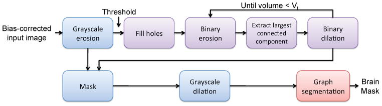
RATS consists of a series of grayscale (blue) and binary (purple) morphological operators, which create an initial surface for the graph-based segmentation algorithm.
2.1. Mathematical morphology for initial surface extraction
The goal of the first stage of the RATS algorithm is to create a good initial surface for the graph search stage. A good initial surface, in this context, needs to be somewhat close to the desired surface, topologically represent the brain to be segmented, and the surface must have well-behaved normals. We propose to use a carefully designed series of grayscale and binary mathematical morphology operators to extract such a surface.
We start by performing a grayscale erosion for smoothing the image while emphasizing the low intensity areas. Next we apply a lower-threshold to the grayscale image to generate a binary mask. We observe that the simple thresholding for converting the grayscale image into a binary mask leads to an excessive amount of structural defects. This can be remedied by filling in the holes fully contained inside the current mask (as opposed to handles or tunnels that are connected to the background). The filled image is morphologically opened with increasingly larger structuring elements until the mask size is within the desirable range. This range is characterized by a single upper boundary on the desired volume. We constrain the binary dilation step of the open operator to the largest connected component of the binary erosion result to get rid of spurious components. We use the binary mask thus computed to constrain the grayscale-eroded image; the final step consists of grayscale-dilation to preserve the size of the brain.
Formally, using the notation IC for complement of binary image I, ⊝ and ⊕ for morphological erosion and dilation Sonka et al. (2008), ∪ for set union, ∩ for masking a grayscale image with a binary image, and given the raw grayscale image I, we define:
| (1) |
| (2) |
| (3) |
| (4) |
| (5) |
| (6) |
where K1 and K2 are ball-shaped structuring elements, threshold[I, x] is the result of thresholding an image I at intensity x, and the LCC[I] operator returns the largest connected component of a binary image I. K2 is selected to be the smallest possible ball-shaped structuring element such that the volume of Imask is less than a volume threshold Vt.
2.2. Graph search for surface optimization
The brain mask extracted using the techniques described above is typically very close to the exact brain boundary but not necessarily on it. To improve the accuracy of the segmentation, we use this brain mask (IMM defined above) as input to a LOGISMOS-based graph segmentation algorithm (Li et al., 2006) which allows us to extract the optimal 3D surface (Yin et al., 2010) given an appropriate cost function. Briefly, we first convert the initial segmentation into a surface mesh using marching cubes and decimate it to a target number of vertices. Each vertex of this mesh is then used to create a column for the graph using the electric lines of force (ELF) to ensure the columns do not intersect each other (Yin et al., 2010). Employing an appropriate cost function along these columns, graph optimization yields the desirable brain surface.
As in (Yin et al., 2010), we introduce nodes along each “column” of the graph, which corresponds to the vertices of the initial segmentation mesh. Intra-column arcs are introduced between each consecutive pair of nodes in a particular column to represent the cost associated with each node; inter-column arcs are introduced between nodes of neighboring columns to enforce smoothness of the final segmentation. However, unlike in (Yin et al., 2010), we define this smoothness constraint based on image-space similarity rather than column-space similarity. Formally, for each edge (vi, vj) in the initial surface mesh, an arc is introduced from each node Va ∈ col(vi) to Vb ∈ col(vj) and from each node Va ∈ col(vj) to Vb ∈ col(vj), where a − b = Δij. The original LOGISMOS (Yin et al., 2010) sets Δij = Δ to a global constant; instead, we determine Δij = arg mina∈col(vj) || vi,0 − vj,a||, where vi,0 is the graph node based on the original surface for column i and vj,a is the ath node in column vj. Intuitively, this corresponds to shifting the origin of each column to best match the origin of the neighboring column. This relaxes the requirements for initial segmentation quality: even if the initial surface is not smooth and has bumps, the final surface will be smooth. Note that using varying smoothness constraints across the surface was first suggested in (Garvin et al., 2009), where these constraints were learned from a training set.
For the rat brain extraction task, we use a mixture of the local image gradient magnitude and signed directional change in image intensity as the cost function, since the desired target surface lies on low intensity areas with a strong gradient. The signed directional change term, which is simply the intensity difference between the two consecutive nodes along the graph column helps distinguish between internal edges (which may be in arbitrary directions) and the true boundary, as well as between the brain-air interface vs. the air-skull interface. The two cost functions are combined by a weighted sum (c = cgradient + α * cintensity).
3. Experimental Methods
3.1. Dataset
To illustrate the performance of our proposed algorithm, we have used two separate datasets.
The first dataset was a collection of in vivo T1-weighted images of 22 adult female Sprague-Dawley rats, acquired with a 9.4 T Bruker scanner using a surface coil, with isotropic 150 μm resolution. Scan time was approximately 40 minutes per subject.
The second dataset was the publicly available Brookhaven in vivo dataset, consisting of T2-weighted images of 12 C57 male adult mice (Ma et al., 2008). The scans were acquired using a 9.4 T Bruker scanner at 100 μm isotropic resolution. Scan time was approximately 2.8 hours per subject. Since the public dataset had incomplete files/segmentations for 2 subjects, these had to be excluded and the evaluation was limited to 10 subjects.
All images were bias-corrected for field inhomogeneities using N4ITK (Tustison et al., 2010) using publicly available software1, and the resulting bias-corrected images were used as input to all three evaluated algorithms.
3.2. Compared methods
We have compared RATS to the two most prominently used methods in the community: the atlas-based tissue classification algorithm (Lee et al., 2009) and the pulse-coupled neural network (PCNN) algorithm (Chou et al., 2011). We obtained the implementations of these methods from the respective authors; the PCNN implementation is also publicly available.2 The RATS implementation was written in C++ using the publicly available ITK3 and VTK4 libraries. The binaries of our implementation will be made available to the rodent research community via our website5 and user support will be provided upon request to the authors.
For the atlas-based tissue classification algorithm, we used a publicly available6 adult rat brain atlas (Rumple et al., 2013) for the rat dataset, and the publicly available Brookhaven C57 atlas for the mouse dataset. From the rat DTI atlas, the mean diffusivity (MD) was used as the registration target. The registration step used mutual information as the similarity metric in an attempt to minimize this difference in contrast.
For the RATS algortihm, we set K1 to have a diameter of 3 voxels, which is roughly twice the expected width of the gap between the brain and non-brain tissue. For simplicity, the K1 diameter was chosen as a multiple of the image resolution. The number of vertices was empirically set to 2000 for both datasets.
The values for Vt, T and α were set based on a quick inspection of the size and intensity profile of the first image in each dataset (i.e. separately for rats and mice, but consistent within each dataset). For the T1-weighted rat dataset, we chose the values Vt = 1650 mm3, T = 500, and α = 5, and we used the same parameter values for the entire dataset without having to resort to fine-tuning. The T2-weighted mouse dataset had a stronger gradient magnitude between the brain and non-brain regions, and we have chosen to simply rely on this magnitude, by setting α = 0. The intensity threshold was simply set to the average intensity in the entire image. The volume parameter was set to Vt = 380 mm3 (note that the mouse brain is much smaller than the rat brain).
3.3. Evaluation criteria
To quantitatively evaluate the performance of RATS, we report the similarity of the brain segmentation results generated by each method and the ground truth. To obtain the independent standard for the rat dataset, the rat images were first skull-stripped using the atlas-based stripping algorithm (Lee et al., 2009). The atlas-based stripping results were manually cleaned up by an anatomical expert, and these results were used as ground truth for the evaluation. For the mouse dataset, 20 manually segmented ROI’s, including the neocortex, subcortical structures, the brainstem and the cerebellum are publicly available; we used the combination of these ROI’s as the ground truth skull-strip mask for this dataset.
For quantitative analysis, we used the Dice ( ) and Jaccard ( ) indices as well as the maximum Hausdorff distance (max{h(A, B), h(B, A)} where h(A, B) = maxa∈A minb∈B ||a − b||). We additionally report computation time for each method. Single-tailed paired t-tests were used for statistical comparison, with 0.05 significance threshold.
4. Results
Figures 2 and 3 give the performance summary of RATS compared to the atlas-based method and PCNN for the rat and mouse datasets, respectively. For both datasets, in all reported measures, RATS performed significantly better (p < 0.05) than the other two methods. In particular, the atlas-based tissue classification had extremely poor results for 3 images from the rat dataset due to inaccurate rigid registration; RATS performs significantly better than the atlas-based method even when these three cases are excluded from analysis (the average values for the atlas method becomes 0.91, 0.83 and 36.5 for Dice, Jaccard and Hausdorff measures, respectively, and p ≪ 0.001 for all three when compared to RATS).
Figure 2.
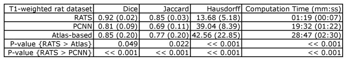
Segmentation performance for RATS and atlas-based tissue classification on the T1-weighted in vivo rat dataset. The values reported are the average (standard deviation). “RATS > Atlas” and “RATS > PCNN” should be interpreted as better, i.e. higher Dice and Jaccard indices and lower maximum Hausdorff distance and computation time. RATS performs significantly better than both the other methods, for all measured criteria.
Figure 3.
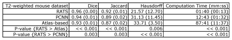
Segmentation performance for RATS and atlas-based tissue classification on the T2-weighted in vivo mouse dataset. The values reported are the average (standard deviation). “RATS > Atlas” and “RATS > PCNN” should be interpreted as better, i.e. higher Dice and Jaccard indices and lower maximum Hausdorff distance and computation time. RATS performs significantly better than both the other methods, for all measured criteria.
Fig. 4 illustrates the best, worst and typical results on the T1-weighted rat dataset, using all three evaluated algorithms. Note that while all the contours are shown on the same coordinate system, the atlas-based tissue classification approach required pre-alignment to the atlas space, unlike RATS and PCNN. PCNN has completely failed to recover the olfactory bulb and piriform cortex in all cases for this dataset; these regions have a very inhomogeneous appearance in the T1-weighted imagery due to the veins that become visible. The atlas-based method is missing most of the brainstem, which is to be expected since the atlas is based on postmortem samples, where a varying portion of the brainstem is missing, resulting from the guillotine placement prior to fixation. RATS achieved a satisfactory segmentation for all the subjects with minor defects typically near the olfactory bulb region. Fig. 5 shows 3D renderings of the brain segmentations for the worst-case subject, further illustrating these observations.
Figure 4.

Typical segmentation comparison for the T1-weighted in vivo rat dataset: green: ground truth, yellow: RATS, red: atlas-based, pink: PCNN. The boundaries are made thicker for visibility. Top: best case, middle: typical case, bottom: worst case. Note that PCNN is missing the olfactory bulb and surrounding areas even in the best case. The atlas-based approach is often missing a significant chunk of the brainstem. RATS achieves satisfactory results even in the worst case, with minor defects near the olfactory bulb.
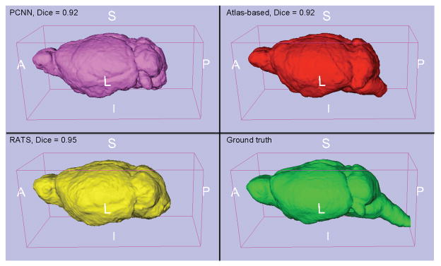
Figure 5.
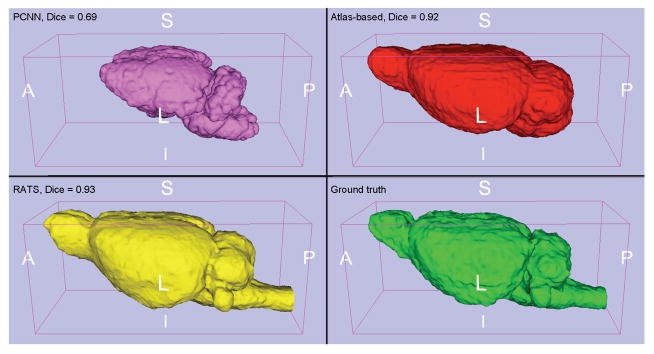
3D brain segmentation on the worst-case subject for the T1-weighted in vivo rat dataset: pink: PCNN, red: atlas-based, yellow: RATS, green: ground truth. PCNN is entirely missing the olfactory bulb and surrounding frontal regions. Additionally, both PCNN and the atlas-based approach are missing significant chunks of the brainstem. RATS produces near-perfect segmentation even for this challenging image. The “worst” subject was chosen as the subject that had the lowest Dice score average over the three methods. The cases where the atlas method had extremely poor performance due to registration failure were excluded from this consideration.
Similarly, Fig. 6 illustrates the best, worst and typical results on the T2-weighted mouse dataset, using all three evaluated algorithms. In this dataset, all three methods produce usable masks, even though RATS recovers the most of the brainstem and is significantly more accurate according to all quantitative metrics. Fig. 7 shows 3D renderings of the brain segmentations for the worst-case subject.
Figure 6.

Typical segmentation comparison for the T2-weighted in vivo mouse dataset: green: ground truth, yellow: RATS, red: atlas-based, pink: PCNN. The boundaries are made thicker for visibility. Top: best case, middle: typical case, bottom: worst case. All three methods produce decent results; however, the brainstem region is observed to have very low signal, causing problems for all methods, to varying degrees. Additionally, the atlas-based method is observed to suffer from inaccurate registration. RATS produces near-perfect results with the exception of the brainstem region and reaches significantly more accurate segmentations compared to the other two methods.
Figure 7.
3D brain segmentation on the worst-case subject for the T2-weighted in vivo mouse dataset: pink: PCNN, red: atlas-based, yellow: RATS, green: ground truth. All three methods produce decent results; however, the brainstem has a strong intensity artifact for this subject, causing problems for all methods to varying degrees. The “worst” subject was chosen as the subject that had the lowest Dice score average over the three methods.
It is particularly noteworthy that RATS took less than 2 minutes per subject for all cases on a standard desktop computer (Intel i7 processor, 2.8GHz, 8 GB RAM), whereas the atlas-based method took approximately half an hour for the rat dataset and 1.5 hours for the mouse dataset per subject. PCNN took 10 to 20 minutes. RATS achieves significantly improved segmentation results in a fraction of the computational time required by existing algorithms. The computation times reported do not include the bias field correction with N4ITK, which is considered as a pre-processing step to all three algorithms.
5. Discussion
The presented results indicate that RATS is a robust and computationally efficient method for accurate rodent brain skull-stripping even in challenging data. Existing rodent skull-stripping methods struggle with low-SNR images with relatively low contrast between brain and non-brain regions, which is often the case in T1-weighted images. This is an even more pronounced problem in live scans in which SNR is low due to limited scan time and the images often have motion and pulsation artifacts. Through a two-stage approach, RATS provides a consistent solution for accurately extracting the brain in a fraction of the computational time of existing methods.
RATS works better than existing methods because it explicitly exploits the knowledge of anatomy of the rodent brain, rather than trying to adapt a general-purpose segmentation method. The initial mathematical morphology step is designed to address particular properties and specifics of the rodent brain anatomy and its appearance on MR images. This also helps set RATS aside from other general-purpose mathematical morphology methods for brain extraction. For example, we observe that many regions inside the brain have low-intensity patches compared to the cortical gray matter, such as the ventricles in T1 images and the white matter in T2 images; these regions get incorrectly thresholded away, which would have made it impossible to accurately recover the whole brain in the subsequent steps that depend on morphological opening without changing the topology of the brain. To remedy this issue, we have introduced a hole-filling step. Our method is grossly insensitive to image artifacts that often plague high-field MR imagery, thanks to the smoothness constraints introduced by the graph-based segmentation step. This step also guarantees a globally optimal segmentation of the brain with respect to the employed cost function.
The robustness of RATS is clearly illustrated in the worst-case performance. For the subject with lowest SNR (8.84) in the T1-weighted dataset, the atlas-based algorithm had a Dice coefficient of 0 (rigid registration completely failed), PCNN had a Dice coefficient of 0.52 whereas RATS achieved a Dice value of 0.85. Additionally, the atlas-based method had very low performance for 3 subjects from the T1-weighted dataset (out of 22) due to visibly poor rigid registration. It is particularly noteworthy that the atlas-based method had these problems even though an unusually well-matched atlas was available for our dataset - the atlas was also built using Sprague-Dawley rats, exactly the same age (postnatal day 72) and scanned with the same scanner. This underlines one of the shortcomings of this method: the success rate is strongly dependent on availability of an external atlas, and even a quite close match might lead to failed segmentations in some cases. In practice, one can either exclude these subjects, or manually initialize the registration, or manually correct the mask as a post-processing; all three of these options are less than ideal, introducing potential selection bias. RATS segmented all tested brains with satisfactory accuracy without a need for such user interaction. It should be noted that, since the Brookhaven mouse dataset was acquired with the intention of inclusion in an in-vivo atlas, the scans had much longer acquisition times than the rat dataset (about 4 times longer for comparable matrix size), and thus has higher SNR overall. Specifically, with the SNR computed according to (Firbank et al., 1999), the Brookhaven mouse dataset had an average SNR of 25.51 (standard deviation: 5.95), while the rat dataset had an average SNR of 15.31(standard deviation: 3.73). The reduced performance of PCNN and the atlas-based approach in the rat dataset is partially attributable to the reduced SNR of this dataset. RATS produces accurate segmentation even in this very challenging dataset.
It is noteworthy that researchers often shy away from using T1-weighted protocols for rodent brain imaging due to low contrast between brain and non-brain tissue to avoid anticipated skull-stripping problems. The low contrast is in particular a problem for the PCNN method, which relies on the strong intensity differences between the cortex and non-brain tissue to achieve good segmentation; in the T1-weighted dataset, the average Dice index for PCNN was 0.81, which is a sharp decline from the 0.94 average it achieved in the T2-weighted dataset. Despite these issues, T1-weighted protocols often provide higher contrast between white matter and gray matter regions, which are often the true endpoints of analysis. Unlike currently existing methods, RATS allows the researchers to choose T1-or T2- weighted images by providing a means to strip away unwanted non-brain tissue; this means the choice of scan protocol can be based on the target endpoints of the study rather than ‘logistic’ problems of preprocessing.
Note that RATS only has five parameters. These all have intuitive interpretations, and the algorithm is not overly sensitive to the exact value of these parameters: the same set of parameter values were successfully used for the entire dataset. In practice, users may need to adjust these parameters once per study based on the acquisition protocol, which affects the intensity profile, and the age/species/strain of the animals, which affects the expected brain sizes.
For the mathematical morphology step, the three employed parameters are the size of K1, the initial intensity threshold T, and the volume threshold Vt. K1 size is directly related to the expected width of the gap between brain and non-brain tissue. Given the excellent robustness of the RATS algorithm on datasets from two different species with a single setting for this parameter, we do not anticipate a need for tuning the K1 size, except potentially to adjust to a dramatically different voxel size. The volume threshold Vt and the intensity threshold T can be set based on the expected brain size and intensity profile of the image, which should be consistent for a dataset acquired with the same scan protocol. We set these values empirically based on the a quick visual inspection of a single image from each set of T1 or T2 data. As such, the same values were employed for the entire T1 or T2 dataset.
The two parameters of the graph-search step are the number of vertices and the relative weight α. Our preliminary results indicate RATS is quite insensitive to the setting of the number of vertices within reasonable range, with the Dice coefficients only varying by about 0.01 for numbers of vertices of 1000, 1500, 2000, 5000, and 10000. The α parameter indicates the relative weight of the edge magnitude and intensity of the image; for datasets with relatively strong gradient magnitude and/or high SNR values, the edge magnitude alone may be used by setting α = 0, as was demonstrated in the T2-weighted mouse dataset.
An important consideration is the smoothness constraints for the graph-based segmentation step. While the image-space smoothing proposed here somewhat improves segmentation quality, additional improvement of RATS results may be possible by replacing the hard smoothness constraints with soft constraints, as recently proposed in (Song et al., 2013). This approach uses arc-cost rather than node-cost functions in the LOGISMOS-based graph segmentation method and further allows the incorporation of shape and context priors. Adoption of this technique for brain extraction remains as future work.
To illustrate the robustness of RATS, we used two sets of in vivo images, which have lower SNR than postmortem images due to limited scan time and are often prone to motion and pulsation artifacts. The presented results show that RATS produces satisfactory results for both T1- and T2- weighted images. Note that diffusion-weighted scans can also be skullstripped using RATS by simply considering the baseline (B0) image, which is T2-weighted. While the datasets included in the manuscript are all acquired with isotropic resolution, in our anecdotal experience, RATS works well on anisotropic data by carrying out computation in physical space rather than image coordinates. Furthermore, we expect both RATS and the other methods evaluated in this manuscript will have problems with severely dysmorphic anatomy. Because our method does not depend on an atlas with similar appearance (unlike the atlas-based method), and because it provides a potential mechanism for local control of its behavior by introducing regionally changing cost functions (unlike PCNN which does not offer such a mechanism but rather considers the image intensity in a more global manner), we believe it could be adapted to such challenging datasets. However, this investigation remains as future work.
Highlights.
We present a novel method for automatically skull-stripping rodent brain MRI datasets.
Our approach combines mathematical morphology techniques and graph-based segmentation.
We evaluate performance using a T1-weighted rat dataset and a T2-weighted mouse dataset.
Our method achieves significantly more accurate results in significantly less computational time.
Our method performs equally well on T1- and T2- weighted imagery, unlike most existing methods.
Acknowledgments
This research was funded, in part, by NIBIB grant R01EB004640. The acquisition of the rat dataset was funded by NIDA grant P01DA022446.
Footnotes
Publisher's Disclaimer: This is a PDF file of an unedited manuscript that has been accepted for publication. As a service to our customers we are providing this early version of the manuscript. The manuscript will undergo copyediting, typesetting, and review of the resulting proof before it is published in its final citable form. Please note that during the production process errors may be discovered which could affect the content, and all legal disclaimers that apply to the journal pertain.
References
- Chou N, Wu J, Bingren JB, Qiu A, Chuang KH. Robust automatic rodent brain extraction using 3D pulse-coupled neural networks (PCNN) IEEE Trans Image Process. 2011;20:2554–64. doi: 10.1109/TIP.2011.2126587. [DOI] [PubMed] [Google Scholar]
- Firbank MJ, Coulthard A, Harrison RM, Williams ED. A comparison of two methods for measuring the signal to noise ratio on MR images. Phys Med Biol. 1999;44:N261–4. doi: 10.1088/0031-9155/44/12/403. [DOI] [PubMed] [Google Scholar]
- Garvin MK, Abràmoff MD, Wu X, Russell SR, Burns TL, Sonka M. Automated 3-D intraretinal layer segmentation of macular spectral-domain optical coherence tomography images. IEEE Trans Med Imaging. 2009;28:1436–47. doi: 10.1109/TMI.2009.2016958. [DOI] [PMC free article] [PubMed] [Google Scholar]
- Lee J, Jomier J, Aylward S, Tyszka M, Moy S, Lauder J, Styner M. Evaluation of atlas based mouse brain segmentation. Proceedings of SPIE. 2009;7259:725943–9. doi: 10.1117/12.812762. [DOI] [PMC free article] [PubMed] [Google Scholar]
- Leemput KV, Maes F, Vandermeulen D, Suetens P. Automated model-based tissue classification of MR images of the brain. IEEE Trans Med Imaging. 1999;18:897–908. doi: 10.1109/42.811270. [DOI] [PubMed] [Google Scholar]
- Li J, Liu X, Zhuo J, Gullapalli RP, Zara JM. An automatic rat brain extraction method based on a deformable surface model. Journal of Neuroscience Methods. 2013 doi: 10.1016/j.jneumeth.2013.04.011. in print. [DOI] [PubMed] [Google Scholar]
- Li K, Wu X, Chen DZ, Sonka M. Optimal surface segmentation in volumetric images–a graph-theoretic approach. IEEE Trans Pattern Anal Mach Intell. 2006;28:119–34. doi: 10.1109/TPAMI.2006.19. [DOI] [PMC free article] [PubMed] [Google Scholar]
- Ma Y, Smith D, Hof PR, Foerster B, Hamilton S, Blackband SJ, Yu M, Benveniste H. In vivo 3D digital atlas database of the adult C57BL/6J mouse brain by magnetic resonance microscopy. Front Neuroanat. 2008;2:1. doi: 10.3389/neuro.05.001.2008. [DOI] [PMC free article] [PubMed] [Google Scholar]
- Oguz I, Lee J, Budin F, Rumple A, McMurray M, Ehlers C, Crews F, Johns J, Styner M. Automatic skull-stripping of rat MRI/DTI scans and atlas building. Proc SPIE. 2011;7962:7962251–7962257. doi: 10.1117/12.878405. [DOI] [PMC free article] [PubMed] [Google Scholar]
- Rumple A, McMurray M, Johns J, Lauder J, Makam P, Radcliffe M, Oguz I. 3-dimensional diffusion tensor imaging (DTI) atlas of the rat brain. PLoS ONE. 2013;8:e67334. doi: 10.1371/journal.pone.0067334. [DOI] [PMC free article] [PubMed] [Google Scholar]
- Ségonne F, Dale AM, Busa E, Glessner M, Salat D, Hahn HK, Fischl B. A hybrid approach to the skull stripping problem in MRI. NeuroImage. 2004;22:1060–75. doi: 10.1016/j.neuroimage.2004.03.032. [DOI] [PubMed] [Google Scholar]
- Smith SM. Fast robust automated brain extraction. Hum Brain Mapp. 2002;17:143–55. doi: 10.1002/hbm.10062. [DOI] [PMC free article] [PubMed] [Google Scholar]
- Song Q, Bai J, Garvin MK, Sonka M, Buatti JM, Wu X. Optimal multiple surface segmentation with shape and context priors. IEEE Trans Med Imaging. 2013;32:376–86. doi: 10.1109/TMI.2012.2227120. [DOI] [PMC free article] [PubMed] [Google Scholar]
- Sonka M, Hlavac V, Boyle R. Image Processing, Analysis, and Machine Vision. 3. Thomson Engineering; Toronto, Canada: 2008. (1st edition Chapman and Hall, London, 1993; 2nd edition PWS Pacific Grove, CA, 1997) [Google Scholar]
- Tustison NJ, Avants BB, Cook PA, Zheng Y, Egan A, Yushkevich PA, Gee JC. N4ITK: improved N3 bias correction. IEEE Trans Med Imaging. 2010;29:1310–20. doi: 10.1109/TMI.2010.2046908. [DOI] [PMC free article] [PubMed] [Google Scholar]
- Yin Y, Zhang X, Williams R, Wu X, Anderson DD, Sonka M. LOGISMOS–layered optimal graph image segmentation of multiple objects and surfaces: cartilage segmentation in the knee joint. IEEE Trans Med Imaging. 2010;29:2023–37. doi: 10.1109/TMI.2010.2058861. [DOI] [PMC free article] [PubMed] [Google Scholar]