

Abstract
A realistic geometric model for the three-dimensional capillary network geometry is used as a framework for studying the transport and consumption of oxygen in cardiac tissue. The nontree-like capillary network conforms to the available morphometric statistics and is supplied by a single arterial source and drains into a pair of venular sinks. We explore steady-state oxygen transport and consumption in the tissue using a mathematical model which accounts for advection in the vascular network, nonlinear binding of dissolved oxygen to hemoglobin and myoglobin, passive diffusion of freely dissolved and protein-bound oxygen, and Michaelis–Menten consumption in the parenchymal tissue. The advection velocity field is found by solving the hemodynamic problem for flow throughout the network. The resulting system is described by a set of coupled nonlinear elliptic equations, which are solved using a finite-difference numerical approximation. We find that coupled advection and diffusion in the three-dimensional system enhance the dispersion of oxygen in the tissue compared to the predictions of simplified axially distributed models, and that no “lethal corner,” or oxygen-deprived region occurs for physiologically reasonable values for flow and consumption. Concentrations of 0.5–1.0 mM myoglobin facilitate the transport of oxygen and thereby protect the tissue from hypoxia at levels near its p50, that is, when local oxygen consumption rates are close to those of delivery by flow and myoglobin-facilitated diffusion, a fairly narrow range.
Keywords: Convection-diffusion Model, Hypoxia, Oxygen
Introduction
In a previous work3 we presented a method for generating a realistic three-dimensional microvascular geometry model to be used as a framework for solving problems of physiological mass transport. The network structure results from randomly connecting a hexagonal arrangement of parallel capillaries with short perpendicular segments. By matching the network to anatomical measurements found in the literature we construct a model with morphometry statistically similar to physiological networks. We showed that the complex three-dimensional structure of the network can have profound effects on the washout of diffusible substances and that simplified models introduce artifacts that have been misinterpreted in the past. Coupled advection and diffusion in the three-dimensional system result in enhanced dispersion of tracer in the axial direction.
This conclusion is similar to that of Schubert et al.,12,22,32 who reported that the effective axial diffusion coefficient required to reproduce measured tissue oxygen distributions is found to be an order of magnitude higher than the expected molecular diffusion coefficient of oxygen. Herein we extend our previous network model3 to study oxygen transport. Understanding the transport of tracer water and tracer oxygen is important in interpreting the results of positron emission tomography experiments used to discover information related to local perfusion and metabolism in the myocardium.6,7,20 Modeling change in flow and its effect on local bulk oxygen concentration is important in interpreting the physiological significance of blood-oxygenation-level dependent contrast magnetic resonance imaging8,23 and 17O-nuclear magnetic resonance imaging26,42 of the working brain. Here we do not relate our modeling results to a specific experimental measure, but instead use the three-dimensional microvascular network model to study the theoretical effects of the network geometry on the transport of oxygen to the tissue.
Van der Ploeg et al.41 point out that a weak point of the Krogh cylinder model is that it always predicts venous pO2 to be lower than capillary pO2, while in experimental measures venous pO2 can be equal to or slightly higher than average capillary pO2. The discrepancy arises from the fact that in a tissue, venules draining one portion of the capillary bed can be located quite near arterioles feeding an adjacent portion of the capillary bed, resulting in diffusional shunting of oxygen from arteriole to venule. This shunting cannot occur when Krogh cylinders are arranged as solitary, noninteracting blood-tissue exchange units. In fact, Van der Ploeg et al.41 report that a simple compartment model reproduces observed data on oxygen distribution in the working heart more accurately than an axially distributed blood-tissue exchange model. Yet a more physically reasonable approach to this problem is to consider modeling microvascular systems distributed in three dimensions and to quantify the effects of interacting microvessels.
Turek et al.40 adopted the Krogh cylinder model to have a tissue radius that varies linearly along the vessel axis. This “truncated cone model” characterizes the apparently different capillary density observed in arterial and venular regions of cardiac tissue. But it is not clear that a cone is a more realistic functional unit of blood-tissue transport than a cylinder. While the observed variation in density can be taken as evidence that the myocardial capillary network does not consist of a symmetric system of parallel pipes, a cone model accounts only superficially for the variation in capillary density. The variation in density suggests that the complexity of the capillary network is not adequately captured by a model of a single capillary independently supplying a local piece of tissue.
In a pioneering study Popel et al.27 demonstrated that heterogeneity of red blood cell (RBC) flux, variations in hematocrit (Hct) and in local RBC velocities and therefore in discharge hematocrits from capillaries contributed substantially to a heterogeneity in intratissue pO2. This elegant study, using a capillary tissue geometry similar to what we use later, showed pO2's that ranged several fold.
Hsu and Secomb16 developed a Green's function method for simulating the steady-state oxygen distribution in a cuboidal region fed by a vascular network with an arbitrary geometry. An analytic expression of the Green's function for Poisson's equation (steady-state diffusion equation with constant consumption) with Neumann boundary conditions was used. The relative weights of all of the sources distributed along the vessel lengths were solved for iteratively, matching the concentration predicted by the Green's function method to the concentration predicted by the equations of local transport. This method has been applied to tissue supplied by realistic microvascular networks.34,35 The simulations predict a high degree of diffusive exchange between microvessels, with diffusive supply of oxygen by arterioles being more important than advective supply to capillaries. About 86% of the consumption in skeletal muscle is diffusively supplied by arterioles.34 Much of that oxygen is taken up by neighboring capillaries and advected to downstream locations.
The appeal of the Green's function method is that it can be more efficient than a finite element or finite difference schemes.34 Another approach to modeling steady-state oxygen exchange with a complex microvascular structure was introduced by Wieringa et al.43 In their model the network consisted of a system of parallel, hexagonally spaced capillaries connected at regular intervals. This model has the advantage that instead of arbitrarily assigning flows to the vessels, flow is calculated based on a linear pressure-flow relationship. In order to ensure that the governing equations remained linear, hematocrit was held constant throughout the network. Once flows were calculated, the inhomogeneous advection-diffusion problem was attacked using a finite difference method. The problem was simplified by not considering diffusion in the axial direction, considering advective transport in the cross connections to be instantaneous, not considering myoglobin facilitation, and by considering the relationship between hemoglobin saturation and oxygen concentration to be linear.
The method of Wieringa et al.43 was constructed to take advantage of linear governing equations (constant consumption and linear oxyhemoglobin dissociation curve). Therefore, it cannot be applied to a problem involving nonlinear consumption in the tissue. Additional nonlinearities, like those that arise when the facilitated transport of oxygen by myoglobin is allowed, also had to be ignored.
Secomb et al.33 modified the linear method of Hsu and Secomb16 to consider nonlinear consumption associated with Michaelis–Menten kinetics. In doing so, the advantage of the Green's function approach over using finite-difference or finite-element grids is diminished because a volume grid of sources is used to account for nonlinearities. In addition, nonlinear effects of myoglobin-facilitated diffusion were considered by Secomb et al.,34 although the details of the methodology were not presented.
It is important to develop a more general solution method that can include nonlinear metabolic kinetics and myoglobin facilitation in the tissue, and can be applied to both steady-state and time-dependent transport problems. Here we use the microvascular geometry developed in Beard and Bassingthwaighte3 and extend the finite difference method to treat the problem of steady-state oxygen distribution.
Methods
The Network
The details of constructing the network geometry used in this study have been described previously.3 This network geometry is illustrated in Figs. 1 and 2, and is quantitatively in accord with data.2,18 Parallel to the z axis, 16 vessels are arranged hexagonally in periodic domain in the x–y plane (see Fig. 1). These parallel “axial” vessels are connected with “crossconnecting” segments that link nearest-neighbor axial vessels at random locations throughout the network (see Fig. 2). A source for arterial inflow occurs at z=500 μm and the venular outflow sinks occurs at z=25 μm and at z=975 μm (see Fig. 2).
FIGURE 1.
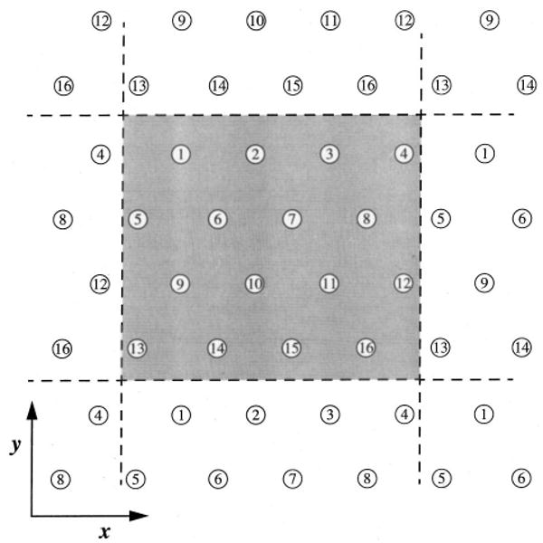
Hexagonal distribution of axially aligned segments. The network is modeled as a periodic arrangement of 16 axial segment positions in the x–y plane. The intercapillary distance used for the calculation was 30 μm.
FIGURE 2.
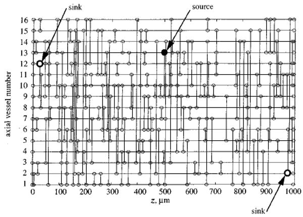
Topology of a network generated by randomly placing 160 crossconnecting segments between nearest neighbor axial vessels. The axial vessel number (see Fig. 1) is plotted vs the axial position. Nodes are indicated as small circles; large filled circle indicates arteriolar source; large open circles indicate venular sinks.
The network geometry is considered to be periodic in the z direction, and therefore the z= 1000 μm position of each axial vessel is topologically connected to the z=0 μm position. The network is considered to be periodic in the x and y directions by allowing crossconnections to occur across the dashed lines in Fig. 1, for example between axial vessels number 1 and number 14. The three-dimensional structure of a realization of the network is rendered in Fig. 3. Shown in the upper panel are the 16 axial vessels along with the associated crossconnecting segments. The lower panel shows a detail of the network.
FIGURE 3.
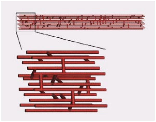
Three-dimensional rendering of capillary network. Sixteen axially aligned vessels are connected by 160 randomly placed cross connecting segments. A detail of the network is shown in the lower panel.
A linear model is used to solve for the flows in the capillary network. Denoting the pressure at the ith node in the network by Pi and the pressure at neighboring nodes by Pj, we have the following flow conservation equation at each node:
| (1) |
where we assume that the conductivity of the vessel connecting the ith and jth node is inversely proportional to the length of the vessel, Lij. Summation in Eq. (1) implies summation over all neighboring nodes. The conservation law takes on a slightly different form at the arterial input node
| (2) |
where Pin is the input pressure, Lin-j is the length of the segment connecting the input node to the jth node and Fin is the input flow. If we force the system by specifying Fin, the pressures at the output nodes can be set to any arbitrary value and Pin treated as an unknown. The normalized nodal pressure in Eqs. (1) and (2) has units of flow times length since these equations are normalized to constant diameter and blood viscosity. For the simulations reported here we use an arterial inflow of 1 mlmin−1 per cubic centimeter of tissue, which corresponds to Fin=2.08× 105 μm3s−1 for the computational volume described later.
This treatment of microvascular flow ignores local variations in vessel diameter and variations in hematocrit that arise at bifurcations. Vessel diameter and hematocrit are treated as constant (and hence, effective viscosity remains fixed), and therefore the earlier equations governing the flow distribution are linear and the constant vessel diameter and hematocrit do not influence the resulting flow distribution. We fix the output nodes at a common (arbitrary) ground pressure, force the system by specifying Fin, and solve for the flow throughout the network.
Using more complex nonlinear hemodynamics equations—such as empirical effective viscosity and phase separation laws29—results in a quantitatively different but qualitatively similar flow distribution (results not shown). For the results described later we use the simple linear equations given earlier since the more complex treatment is not found to influence our main results or conclusions on oxygen transport in the tissue.
Advection, Diffusion, and Reaction of Oxygen in the Myocardium
Equations of Mass Transport
The system is composed of two regions, an advective region not consuming oxygen, capillaries containing hemoglobin, and a stagnant extravascular region, the tissues where there is oxygen consumption and facilitated diffusion of oxygen by myoglobin. (No interstitial space is modeled.)
Mass transport by advection and diffusion in the capillary is governed by
| (3) |
where CT is the total (free plus bound) oxygen concentration
| (4) |
and ν⃗ is velocity of the blood, C is the free oxygen concentration, CHb is the hemoglobin concentration in a red cell, SHb is the oxygen saturation of hemoglobin, Dc is the free oxygen diffusion coefficient, H is the hematocrit, and x⃗ indicates position. Consumption is not considered to occur inside the capillary. A factor of 4 appears multiplying the second term in Eq. (3) because each hemoglobin molecule contains four binding sites for oxygen. We consider the binding of oxygen to hemoglobin to be in equilibrium and to be governed by the Adair equation
| (5) |
where α = 0.00135 mM mm Hg−1 is the solubility coefficient of oxygen and a1 =0.01524, a2 = 2.7 × 10⁻⁶, a3 = 0 (for human), and a4 = 2.7 × 10⁻⁶.
All concentrations (C, CHb, and CT) in Eq. (3) have units of moles per unit volume of blood. Thus erythrocytes are not explicitly modeled and the hemoglobin binding sites are assumed to be homogeneously distributed throughout the capillary. The model ignores the two-phase (erythrocyte and plasma phases) nature of the blood, and therefore the intraluminal resistance to oxygen transport, especially at low hematocrits, is underestimated.9,10,14,15 Yet the focus of this investigation is on the distribution of oxygen on the size scale of a network of several microvessels and not on the microscopic concentration profiles within microvessels. The discrete nature of erythrocytes, which is ignored by our continuum model, is assumed to have only secondary effects on the oxygen distribution on the size scale of the network/tissue system which we study, a reasonable assumption at normal hematocrits.
Transport outside of the capillary is governed by
| (6) |
where CMb is the bulk tissue concentration of myoglobin, DMb is the diffusion coefficient of myoglobin in the tissue, and G is the rate of oxygen consumption. Free oxygen is assumed to diffuse isotropically and homogeneously throughout the vessels and the tissue, with a continuous concentration across the vessel walls. Myoglobin, on the other hand, is restricted to the extravascular region and a no-flux condition is imposed on SMb at vessel walls. This simplistic two-region approach ignores the fact that the distance from the capillary blood to the Mb inside the cardiomyocytes is perhaps 0.3–0.5 μm, namely the thickness of an endothelial cell plus that of the thin layer of ISF separating the endothelial cell from the myocyte. Here, the total oxygen concentration is given by
| (7) |
The binding of oxygen to myoglobin is considered to be governed by the two-state equilibrium expression
| (8) |
where C50 is the free oxygen concentration at 50% saturation. The value for C50 was taken as 2.5 Torr, slightly higher than the value of 2.39 Torr found by Schenkman et al.30 for Mb in solution of pH 7.0 and 37 C, in the direction of lower pH or slightly higher temperature.
The kinetics of uptake of oxygen by cytochrome oxidase is modeled by Michaelis–Menten enzyme kinetics
| (9) |
where Gmax is the maximum rate of consumption and Km is the apparent Michaelis constant for oxygen conversion by cytochrome oxidase, and was taken to be 0.07 μM or a p50 of 0.052 mmHg. (pO2, Torr, equals the O2 concentration, molar, divided by α, the solubility of O2 in water at 37 C, which is 1.35 μM Torr−1) Equation (9) gives a practically constant consumption when the p O2 is higher than the C50 for Mb since it is 35 times the Km; consumption goes linearly to zero as the concentration gets small.
We consider a computational domain of cuboidal dimensions of 120×120 × 1000 μm, on which we apply a finite-difference approximation using a hexagonal grid with resolution 5 μm to solve the steady-state equations for oxygen transport. This grid resolution is sufficient for describing the concentration field on the size scale of our multicapillary network model, but does not resolve intracapillary radial concentration profiles. The numerical methodology and accuracy assessment are detailed in the Appendix. All of the parameters used for model simulations are listed in Table 1.
TABLE 1. Parameters used for model simulations.
| Parameter | Description | Value | Reference |
|---|---|---|---|
| F | Arterial inflow per unit mass of tissue | 1 ml min−1 g−1 | |
| Gmax | Maximum rate of oxygen consumption | 3–10 μmol min−1g−1 | |
| Km | Michaelis constant | 1.0×10⁻⁷ M | |
| Hct | Hematocrit | 0.45 | |
| D0 | Free oxygen diffusion coefficient | 2.41 ×10⁻⁵ cm2s−1 | 5 |
| DMb | Myoglobin diffusion coefficient | 2.2×10⁻⁷ cm2s−1 | 25 |
| CHb | Red cell hemoglobin concentration | 5.3×10⁻³ M | |
| CMb | Tissue myoglobin concentration | 0.1 ×10⁻³ M | 44 |
| α | Oxygen solubility coefficient | 1.35×10⁻⁶ M mm Hg−1 | 5 |
Results
Predicted Steady-State Concentrations
For solutions to the steady oxygen transport problem, a finite difference scheme is applied on a grid with 5 μm resolution and 24×24×200 = 115,200 nodes (see the Appendix for details). Solutions for the nonlinear oxygen transport problem were obtained on a Sun Sparcstation 5 in anywhere from about 10 to 100 min. The rate of convergence of the method depends on the minimum value of pO2 predicted in the tissue. As the tissue become hypoxic, nonlinearities dominate and successive overrelaxation becomes unstable. So an accurate solution requires more iterations for higher levels of consumption.
Representative simulation results are illustrated in Fig. 4 for Gmax=5 μmol min−1 g−1 and CMb=0.5× 10⁻³ M. Input free oxygen concentration is set to 0.135 mM (100 mmHg). On the left side, oxygen tension is mapped in the x–y plane at z=0, 250, and 500 μm using the color scale shown in the figure. The image on the right side depicts oxygen tension in a slice through the x–z plane. The maximum concentration occurs near the arterial inflow at x=0 μm and z=500 μm. In the x–y slices, the vessel locations are apparent as local maxima in oxygen tension.
FIGURE 4.
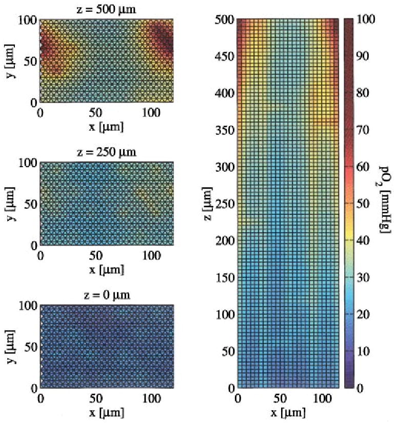
Images of oxygen tension in various slices through the tissue. On the left are slices in the x–y plane at z=0, 250, and 500 μm. The image on the right is a slice in the x–y plane. For these results, CMb=0.5×10⁻³ M and Gmax =5 μmol min−1g−1. Note that pO2 gradients are evident within capillaries and that there is no sudden drop in pO2 at the capillary wall since the wall is so permeable to O2.
In Fig. 5 we compare the intravascular total oxygen concentration predicted by the three-dimensional network model to the total oxygen concentration predicted by an axially distributed model. Oxygen concentration in each axial vessel is plotted versus axial position along with the concentrations predicted by an axial model (for example, see Refs. 6 and 19). For the axially distributed model, the steady-state total oxygen concentration linearly decreases from the arterial end of the capillary to the venous end. We note that the intravascular concentration profiles predicted by the three-dimensional network model tend to decay in a manner similar to those predicted by the axial model, yet differ considerably from the straight lines predicted by the simpler model.
FIGURE 5.
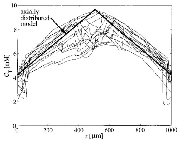
Total intravascular oxygen concentration in each axial vessel is plotted vs axial position. Also plotted is the concentration predicted by an axially distributed model and a compartmental model. Here, CMb=0.5×10⁻³ M and Gmax = 5 μmol min−1 g−1.
Concentration profiles in the tissue are shown in Fig. 6. The thick solid line represents the mean tissue pO2 in the x–y plane as a function of axial position. The maximum occurs near the arterial inflow (z=500 μm). The dashed lines represent the mean ± one standard deviation. The thin lines are the maximum and minimum values of pO2 in the x–y plane at each axial position.
FIGURE 6.
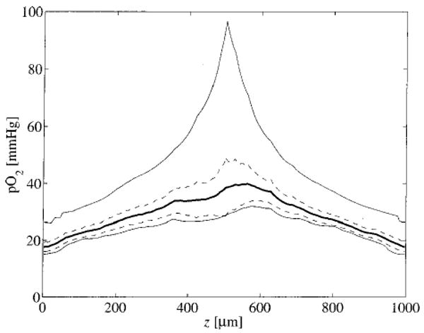
Tissue pO2 in the x–y plane is plotted as a function of axial position. The dark solid line represents the mean pO2 in the x–y plane at each axial position. The dashed lines represent the mean plus and minus one standard deviation. The thin lines are the maximum and minimum values of pO2. For these results, CMb=0.5–10−3 M and Gmax=5 μmol min−1 g−1.
Effects of Increasing Oxygen Consumption
To calculate the probability density function of tissue oxygen tension, we generated ten independent realizations of the random capillary network, and solved the steady oxygen transport equations for each realization for several different values of Gmax. It was found that ten realizations were sufficient for convergence of the density function. The results are summarized in Fig. 7, where the probability density functions of tissue pO2 predicted by the model are shown for Gmax=3, 5, and 7 μmol min−1 g−1. As Gmax increases the probability density function tends to retain its shape while shifting to the left along the pO2 axis. When Gmax is high enough to induce hypoxia, consumption in the hypoxic regions decreases according to Eq. (9) and the shape of the distribution changes (long dashes, Gmax=7 μmol g−1 min−1).
FIGURE 7.
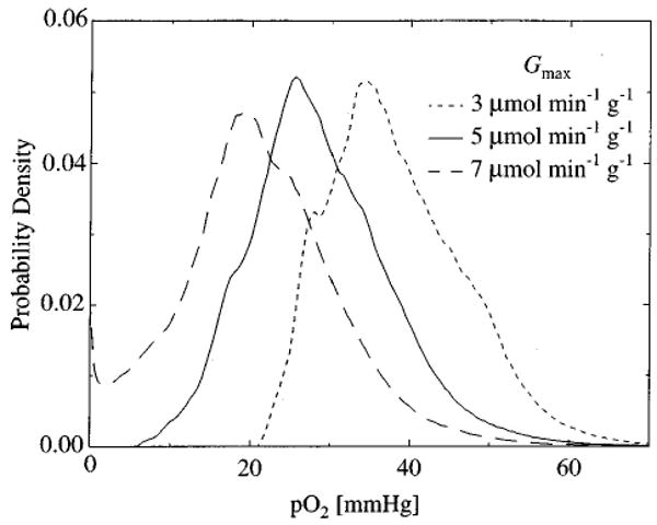
The probability density of tissue pO2 predicted by the model is plotted for various values of Gmax. As Gmax increases, tissue pO2 decreases. When Gmax =7 μmol min−1g−1, a fraction of the tissue is hypoxic. These results are for oxygen concentration in ten independent realizations of the microvessel network computed using CMb = 0.5×10⁻³ M.
Myoglobin Facilitation
We expect that hypoxia should, to some degree, be alleviated by the presence of myoglobin. The distributions shown in Fig. 7 were calculated from ten realizations of the network using a fixed myoglobin concentration (CMb= 0.5× 10⁻³ M). In the upper panel of Fig. 8 the minimum tissue pO2 from a single realization of the microvessel network is plotted as a function of tissue myoglobin concentration for various values of Gmax. As CMb increases the relative importance of myoglobin in transporting oxygen to the tissue increases and minimum pO2 increases. For Gmax=7.6 μmol min−1 g−1, pO2 ranges from a value well below the cytochrome oxidase Km, about 0.07 mmHg, to a value well above the Km as CMb increases from 0 to 1.0 mM. Another way to visualize this effect is illustrated in the lower panel of Fig. 8 by plotting the minimum value of G/Gmax occurring in the tissue as a function of CMb. Values of G/Gmax much below 1.0 indicate hypoxia.
FIGURE 8.
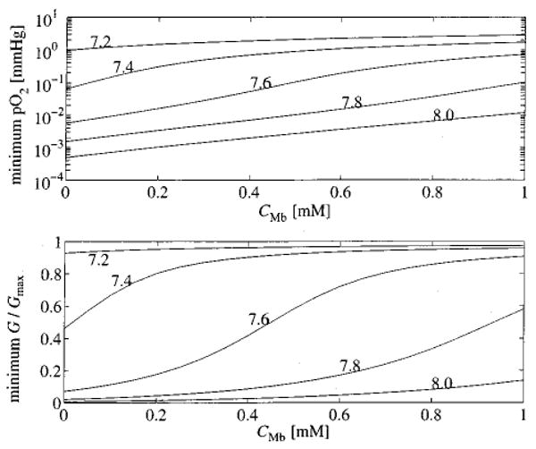
The effectiveness of myoglobin facilitated transport at preventing hypoxia is investigated for various concentration of myoglobin. In the upper panel, the minimum pO2 in the tissue is plotted as a function of the concentration of myoglobin in the tissue. Each curve is labeled with the value of Gmax in μmol min−1 g−1 used in the computation. The lower panel plots the minimum oxygen consumption normalized to Gmax as a function of CMb.
In Fig. 9, the minimum value of G/Gmax obtained in the tissue for a single realization of the network is plotted as a function of Gmax. The resulting sigmoidal curves are shifted to the right as myoglobin concentration is increased, indicating that myoglobin-facilitated transport does reduce hypoxia, but suggesting that it is effective only over a narrow range of consumption rates.
FIGURE 9.
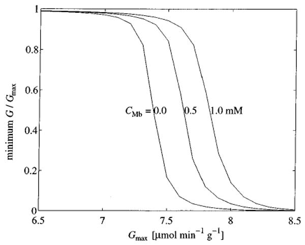
Minimum oxygen consumption as a function of Gmax for various levels of CMb.
Discussion
That the complex vascular geometry influences the transport of oxygen to tissues is well known.28,34,43 Our modeling study of tracer transport in the microvasculature3 revealed that the details of the geometry of the capillary network effects a profound influence on the kinetics of the transport of passive highly diffusible substances. In extending our microvascular network/tissue model to study oxygen transport based on a finite-difference formulation, we have developed a convenient methodology for simulating steady-state oxygen delivery that considers nonlinear binding of oxygen to hemoglobin and myoglobin and nonlinear consumption of oxygen in the tissue. The modeling of the network is inexact, using averages: capillary diameters actually1 range from 2.5 to 7.5 μm with a mean and SD of 5.6 ± 1.3 μm in dog heart, but we used a fixed 5 μm diameter for the modeling. The capillary density used here, 1333 capillaries per mm2, or 16 per 120 by 100 μm cross section, is below the range of 3100–3800 capillaries per mm2 cross section in dog hearts and therefore underestimates the effectiveness of Mb diffusion. Intercapillary distances average 18 μm in heart and about 40 μm in skeletal muscle; in our modeling analysis we used 30 μm. So our example geometric arrangement is a worst case for heart muscle and is a little closer to skeletal muscle.
The studies of Popel et al.27 used 51 μm intercapillary distances compared to our 30 μm; they did not consider the contribution of Mb. Their source of heterogeneity in the oxygen delivery was probabilistic variation in both inflow pO2 and RBC flux, due to variation in hematocrit and oxygen loss in the upstream arterioles. We have modeled neither of these sources of variation but limited ourselves to the consideration of variation in velocities within capillaries and in path lengths taken by the blood in a heterogeneously connected network. While their distributions of pO2 are not too different from ours, we cannot conclude that one approach confirms or denies the other. A more complete consideration of the problem would combine these approaches.
Most previous modeling studies of oxygen transport in complex vascular networks have relied on some linearization of the governing equations. In general, one or more of the following simplifying assumptions has been made: (1) treatment of the oxyhemoglobin dissociation curve as linear; (2) treatment of oxygen consumption using either first or zeroth order kinetics; and (3) ignoring myoglobin facilitated transport. None of these assumptions are valid for the full range of physiologically reasonable flows and consumption.
The recent work of Goldman and Popel,13 on the other hand, is more or less complete in the sense that none of these simplifications is applied. In fact, the Goldman and Popel13 method is more sophisticated than ours because luminal resistance is treated explicitly and it can be applied to more arbitrary vascular anatomies.
It is apparent from Fig. 5 that the steady-state oxygen concentration predicted by the three-dimensional model is more closely approximated by an axially distributed model than by a well-mixed compartment model. This is because a substantial fraction of the oxygen content of blood is extracted as it passes through the microcirculation. The trend for oxygen content to decrease more or less linearly from arteriole to venule is captured by axially distributed models such as that of Li et al.20
The degree of facilitation provided by myoglobin is a function of the diffusion distance and of consumption. Fletcher11 demonstrated, in a model for skeletal muscle using a single capillary-tissue domain with a radius of 30 μm, that the facilitation was maximal in the periphery where the pO2 is in the neighborhood of the p50 of myoglobin for oxygen, and depends therefore on the local consumption of O2 relative to its delivery by diffusion. At higher consumptions the role of Mb will be more important.
It is clear from Fig. 8 that myoglobin can have a significant influence on oxygen transport in our model geometry. With no myoglobin present, oxygen concentration drops well below Km at a Gmax =7.6 μmol min−1 g−1 for a flow of 1.0 ml min−1 g−1, yet the presence of myoglobin relieves the hypoxia. Since the value of consumption at which a region in the tissue becomes hypoxic depends on the flow and on the exact microvascular geometry, the specific value of Gmax=7.6 μmol min−1 g−1 is not of critical importance. It is an important interpretation that a reasonable concentration of myoglobin can bring the tissue out of hypoxia and raise the free oxygen concentration to a healthy level even though the DMb of 2.2× 10⁻⁷ cm2 s−1 is about two orders of magnitude smaller than the tissue diffusion coefficient for free oxygen. This intracellular diffusion coefficient is difficult to estimate precisely in vivo; our chosen value is higher than the 1.7×10⁻⁷ cm2s−1 observed by Jürgens et al.17 in rat diaphragm and lower than the 2.7× 10⁻⁷ cm2s−1 estimated in rat muscle homogenate by Moll.21 Our computer profiles exhibit myoglobin saturation levels similar to those observed in dog hearts by Schenkman et al.31
Yet from Fig. 9 it is apparent that the range of metabolic consumption over which myoglobin facilitation can really prevent hypoxia is fairly narrow. The relatively high estimate of CMb = 1.0 mM results in an increase in the maximum supportable Gmax of less than 10%. These results indicate that metabolic kinetics must be precisely tuned to the effective operating range to take advantage of myoglobin as a transporter of oxygen. An alternative hypothesis to this rather unlikely scenario is that myoglobin acts as an oxygen storage buffer.24 Assuming CMb = 0.5 mM and Gmax=7.6 μmol min−1 g−1, myoglobin-bound oxygen stores would be depleted in about 6 s. Thus, the time scale of effective myoglobin buffering is similar to the time scale of a few heart beats. Perhaps some combination of myoglobin-facilitated transport and myoglobin buffering is responsible for maintaining tissue oxygen concentrations during the temporary decrease in endocardial perfusion realized during systole. This hypothesis can be investigated by incorporating time-dependent behavior into the model.
Takahashi et al.37–39 have studied oxygen uptake and consumption in isolated rat cardiomyocytes by spectrophotometrically measuring myoglobin saturation and mitochondrial NAD(P)H levels at intracellular resolution. They find that when significant gradients in SMb exist—at relatively low extracellular O2 concentration (10–30 mmHg)—oxygen supply and consumption can be suppressed by inhibiting myoglobin facilitation with MaNO2. Note that this experiment39 was deliberately carried out with the system parameters set in the (possibly narrow) range where gradients in SMb exist and myoglobin-facilitated transport is expected to be near maximal. As Takahashi et al.39 point out, it remains to be seen whether a similar state is achieved in the myocardium in vivo. As we have shown, calculations based on our model geometry show that even at artificially high levels of intracellular myoglobin concentration myoglobin acts as a significant carrier of oxygen only over a narrow range of metabolic consumption.
A possibly important factor ignored in our model and in most state-of-the-art mathematical models of oxygen transport in tissue is the heterogeneous distribution of oxygen consumption due to variations in the density of mitochondria within the myocyte. Because mitochondria are preferentially distributed near cell surfaces as well as around the bundles of contractile proteins, the local gradients in cytosolic oxygen concentration near the membrane of a mitochondrion may be larger than those predicted by homogeneous consumption models. Thus, the discrete positioning of the mitochondria undoubtedly steepens the local gradients for oxygen transport and therefore the role of myoglobin-facilitated transport must be at least a little greater than that predicted by the present model.
Acknowledgments
This work was supported by NIH Grant No. RR01243 (National Simulation Resource for Mass-Transport and Exchange).
Appendix: Numerical Methods
Finding the Steady State
Since the axially aligned vessels are hexagonally spaced in the model, it is reasonable to use a numerical scheme which employs a hexagonal grid in the x–y plane (see Fig. 10). In the left panel of Fig. 10 the positions of the axial vessels are denoted by solid circles.
FIGURE 10.
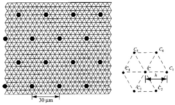
Hexagonal grid used for numerical computation. Concentration at a node is denoted by C. Concentrations in the six surrounding nodes in the x–y plane are denoted by C1–C6.
Notation used for the numerical method is illustrated in the right panel of Fig. 10. Consider a node in the tissue to have concentration C. The six surrounding nodes in the x–y plane are denoted by C1–C6. Nodes are separated by the step size, h. We denote the neighboring concentration in the positive z direction by C7 and the neighboring concentration in the negative z direction by C8. A numerical approximation to the Laplacian operator on the mesh is given later and denoted by L2{C}:
| (10) |
Using this approximation, Eq. (3) can be discretized for the steady state as follows:
| (11) |
where the hemoglobin saturation at a given node is denoted by SHb. Then the neighboring values of saturation are denoted by SHb1–SHb8 in the same manner as the neighboring free oxygen concentrations were defined. We have defined ki as the plasma flow per unit volume entering from the ith node and kei is the red cell flow per unit volume entering from the ith node. Note that the ki will be nonzero only when the ith node corresponds to an upstream vessel location.
Since most of the oxygen in the blood is bound to hemoglobin, and the saturation varies nonlinearly with oxygen concentration, total oxygen concentration (free concentration plus bound concentration) tends to vary more smoothly than free oxygen concentration in a vessel. By posing the finite volume scheme in the vessels in terms of total oxygen concentration instead of free oxygen concentration, the stability of the problem is improved. Rewriting Eq. (11) in terms of CT, we get
| (12) |
where
| (13) |
and H is the hematocrit in the vessel.
We discretize Eq. (6) for the steady state as follows:
| (14) |
where SMb is the myoglobin saturation at a given node and the myoglobin saturation values in the eight surrounding nodes are denoted by SMb1–SMb8. We impose the no-flux boundary to myoglobin diffusion at the vessel wall by setting SMbi = SMb when the ith node corresponds to a capillary.
Before attempting to solve Eqs. (12) and (14) it is useful to nondimensionalize the equations. We can rewrite Eqs. (12) and (14) as
| (15) |
and
| (16) |
after making the following definitions:
| (17a) |
| (17b) |
| (17c) |
| (17d) |
| (17e) |
| (17f) |
| (17g) |
where Cin is the concentration of free oxygen in the arterial input. We solve Eqs. (15) and (16) by initially setting φ= 1 everywhere in the tissue and Φ = 1 + 4CHbH/Cin in every vessel and iteratively determining better approximations to φ and Φ at each of the grid points as outlined later.
Oxygen Concentration in the Tissue
Equation (16) reduces to a quadratic equation in φ that allows us to solve for φ as a function of its neighboring concentrations. For a linear equation this would be equivalent to taking a Gauss-Seidel iteration step36 and we denote this estimate by φGS. Successively choosing the Gauss–Seidel estimate does not always converge for this nonlinear problem so we modify our choice for the estimate of φ〈n+1〉 [estimate at the (n+ 1)th iteration] by
| (18) |
where ω1 is some constant. Then we can calculate an estimate of ψ at the (n+ 1)th iteration by
| (19) |
where C50 is the oxygen concentration at 50% myoglobin saturation.
To efficiently converge to a solution, we must make an appropriate choice of ω1. For symmetric linear systems it can be shown that ω1 must be less than 2 for convergence.36 In this case the system is not symmetric because of the convective terms [in Eq. (15)] in the vessels and is not linear because of the nonlinear consumption and binding to myoglobin. Even so, Eq. (16) is approximately linear for high values of φ and converges for ω1≈ 1.6 when φ≫D and φ≫C50/Cin. When φ is of the same order of magnitude as D or C50/Cin nonlinearities become more important and we find that ω1 must be smaller than 1 to get stable behavior. The value of ω1 depends on the minimum value of φ for a particular solution.
Since we would like to set ω1 as high as possible to converge as quickly as possible, we start with the relatively high choice of ω1 = 1.6 and adjust this value as the computation proceeds and the global minimum of φ is reduced. In fact, Eq. (18) tells us when our current choice of ω1 is too high by predicting a negative value of φ. When this happens ω1 is modified according to Eq. (20) and the computation associated with the nth step is repeated:
| (20) |
Oxygen Concentration in the Vessels
Inside the vessel it is found that nonlinearities dominate and we find that we need to use under relaxation to get convergence.
Once we have completed the calculation of φ〈n+1〉 in the tissue, we can construct a linear system of equations for the total oxygen concentration in the vessel using Eq. (15). If we call the first guess as the total oxygen concentration , then we get
| (21) |
An iterative scheme similar to that used in the tissue is applied
| (22) |
In this case convergence is achieved only if ω2 is less than about 0.025. Typically, convergence requires about 500 iterations.
Once a new estimate of is calculated from Eq. (22), φ(ν+1), the nondimensional free oxygen concentration is found by solving Eq. (17d) for φ(ν+1) where the hemoglobin saturation is given by the Adair equation [Eq. (5)].
Numerical Accuracy
The accuracy of the numerical method is assessed by studying the one-dimensional steady-state reaction-diffusion system described by
| (23) |
over the interval 0<x<L, with Dirichlet boundary conditions
| (24) |
We study this one-dimensional problem because it allows us to refine the numerical method to greater resolution than is possible for two- and three-dimensional problems.
We discretize Eq. (23) as
| (25) |
Choosing the concentration of the end points so as to be sufficiently low (C0 = 5 mm Hg·α) forces the system into the nonlinear regime where the effects of Michaelis–Menten consumption and myoglobin-facilitated diffusion strongly influence the behavior. Plotted in Fig. 11 are the concentration profiles obtained numerically using C0 = 5 mm Hg·α, GMax=2 × 10⁻⁴ Ms−1, and L=30 μm. The value of L is chosen as the radial distance between capillaries in the network model. In Fig. 11 the solid lines correspond to high-resolution converged solutions obtained using h=0.5 μm, for two values of CMb. Solutions obtained using h=5 μm are plotted as solid circles. Clearly the grid resolution of 5 μm is sufficient to describe the concentration profiles for this homogeneous system. However, the 5 μm grid does not resolve the radial intracapillary concentration profiles in the interior of the vessels in the three-dimensional network model.
FIGURE 11.
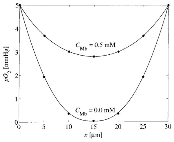
Numerical solutions to Eq. (23). Predicted pO2 is plotted vs x, for h=0.5 μm (solid lines) and h=5.0 μm (circles) for CMb of 0.05 and 0.0 mM. Gmax=2×10⁻⁴ Ms−1.
Note that this one-dimensional application of the numerical approach is not an ideal test for its application to the three-dimensional hexagonal lattice employed for oxygen transport problem. While the hexagonal mesh (Fig. 10) offers the advantage that it is specifically engineered for application to the regular hexagonal arrangement of capillaries which we study, it has the disadvantage that it cannot be refined arbitrarily without changing the anatomy of the vessel network. This is because in cross section each vessel corresponds to exactly one lattice point (see Fig. 10). Recently we have developed a more general methodology which can be applied to networks of arbitrary geometry and is the subject of a forthcoming publication.4 This new method will allow us to incorporate features that are not included in the current work, such as more realistic vessel geometries and finite vessel wall permeabilities.
References
- 1.Bassingthwaighte JB, Yipintsoi T, Harvey RB. Microvasculature of the dog left ventricular myocardium. Microvasc Res. 1974;7:229–249. doi: 10.1016/0026-2862(74)90008-9. [DOI] [PMC free article] [PubMed] [Google Scholar]
- 2.Batra S, Rakusan K. Morphometric analysis of capillary nets in rat myocardium. Adv Exp Med Biol. 1990;277:377–385. doi: 10.1007/978-1-4684-8181-5_43. [DOI] [PubMed] [Google Scholar]
- 3.Beard DA, Bassingthwaighte JB. Advection and diffusion of substances in biological tissues with complex vascular networks. Ann Biomed Eng. 2000;28:253–268. doi: 10.1114/1.273. [DOI] [PMC free article] [PubMed] [Google Scholar]
- 4.Beard DA. Computational framework for generating transport models from databases of microvascular anatomy. Ann Biomed Eng. 2001;29(10):837–843. doi: 10.1114/1.1408920. [DOI] [PubMed] [Google Scholar]
- 5.Bentley TB, Meng H, Pittman RN. Temperature dependence of oxygen diffusion and consumption in mammalian striated muscle. Am J Physiol. 1993;264:H1825–H1830. doi: 10.1152/ajpheart.1993.264.6.H1825. [DOI] [PubMed] [Google Scholar]
- 6.Cousineau DF, Goresky CA, Rose CP, Simard A, Schwab AJ. Effects of flow, perfusion pressure, and oxygen consumption on cardiac capillary exchange. J Appl Physiol. 1995;78:1350–1359. doi: 10.1152/jappl.1995.78.4.1350. [DOI] [PubMed] [Google Scholar]
- 7.Deussen A, Bassingthwaighte JB. Modeling [15O] oxygen tracer data for estimating oxygen consumption. Am J Physiol. 1996;270:H1115–H1130. doi: 10.1152/ajpheart.1996.270.3.H1115. [DOI] [PMC free article] [PubMed] [Google Scholar]
- 8.Ellermann J, Garwood M, Hendrich K, Hinke R, Hu X, Kim SG, Menon R, Merkle H, Ogawa S, Ugurbil K. NMR in Physiology and Biomedicine. New York: Academic; 1994. Functional imaging of the brain by nuclear magnetic resonance; pp. 137–150. [Google Scholar]
- 9.Federspiel WJ, Popel AS. A theoretical analysis of the effect of the particulate nature of blood on oxygen release in capillaries. Microvasc Res. 1986;32:164–189. doi: 10.1016/0026-2862(86)90052-x. [DOI] [PMC free article] [PubMed] [Google Scholar]
- 10.Federspiel WJ. A model study of intracellular oxygen gradients in a myoglobin-containing skeletal muscle fiber. Biophys J. 1986;49:857–868. doi: 10.1016/S0006-3495(86)83715-8. [DOI] [PMC free article] [PubMed] [Google Scholar]
- 11.Fletcher JE. On facilitated oxygen diffusion in muscle tissues. Biophys J. 1980;29:437–458. doi: 10.1016/S0006-3495(80)85145-9. [DOI] [PMC free article] [PubMed] [Google Scholar]
- 12.Gardner JD, Schubert RW. Myoglobin function evaluated in working heart tissue. Adv Exp Med Biol. 1998;454:509–517. doi: 10.1007/978-1-4615-4863-8_61. [DOI] [PubMed] [Google Scholar]
- 13.Goldman D, Popel AS. A computational study of the effect of capillary network anastomoses and turtuosity on oxygen transport. J Theor Biol. 2000;206:181–194. doi: 10.1006/jtbi.2000.2113. [DOI] [PubMed] [Google Scholar]
- 14.Hellums JD. The resistance to oxygen transport in the capillaries relative to that in the surrounding tissue. Mi-crovasc Res. 1977;13:131–136. doi: 10.1016/0026-2862(77)90122-4. [DOI] [PubMed] [Google Scholar]
- 15.Hellums JD, Nair PK, Huang NS, Ohshima N. Simulation of intraluminal gas transport processes in the mi-crocirculation. Ann Biomed Eng. 1996;24:1–24. doi: 10.1007/BF02770991. [DOI] [PubMed] [Google Scholar]
- 16.Hsu R, Secomb TW. A Green's function method for analysis of oxygen delivery to tissue by microvascular networks. Math Biosci. 1989;96:61–78. doi: 10.1016/0025-5564(89)90083-7. [DOI] [PubMed] [Google Scholar]
- 17.Jürgens K, Peters T, Gros G. Diffusivity of myoglobin in intact skeletal muscle cells. Proc Natl Acad Sci USA. 1994;91:3829–3833. doi: 10.1073/pnas.91.9.3829. [DOI] [PMC free article] [PubMed] [Google Scholar]
- 18.Kassab G, Fung YB. Topology and dimensions of the pig coronary capillary network. Am J Physiol. 1994;267:H319–H325. doi: 10.1152/ajpheart.1994.267.1.H319. [DOI] [PubMed] [Google Scholar]
- 19.Krogh A. The number and distribution of capillaries in muscles with calculations of the oxygen pressure head necessary for supplying the tissue. J Physiol (London) 1919;52:409–415. doi: 10.1113/jphysiol.1919.sp001839. [DOI] [PMC free article] [PubMed] [Google Scholar]
- 20.Li Z, Yipintsoi T, Bassingthwaighte JB. Nonlinear model for capillary-tissue oxygen transport and metabolism. Ann Biomed Eng. 1997;25:604–619. doi: 10.1007/bf02684839. [DOI] [PMC free article] [PubMed] [Google Scholar]
- 21.Moll W. The diffusion coefficient of myoglobin in muscle homogenate. Pflugers Arch Gesamte Physiol Menschen Tiere. 1968;299:247–251. doi: 10.1007/BF00362587. [DOI] [PubMed] [Google Scholar]
- 22.Napper SA, Schubert RW. Mathematical evidence for flow-induced changes in myocardial oxygen consumption. Ann Biomed Eng. 1988;16:349–365. doi: 10.1007/BF02364623. [DOI] [PubMed] [Google Scholar]
- 23.Ogawa S, Menon RS, Tank DW, Kim SG, Merkle H, Ellermann JM, Ugurbil K. Functional brain mapping by blood oxygenation level-dependent contrast magnetic resonance imaging. A comparison of signal characteristics with a biophysical model. Biophys J. 1993;64:803–812. doi: 10.1016/S0006-3495(93)81441-3. [DOI] [PMC free article] [PubMed] [Google Scholar]
- 24.Paaske WP, Sejrsen P. Microvascular function in peripheral vascular bed during ischaemia and oxygen-free perfusion. Eur J Endovasc Surg. 1995;9:29–37. doi: 10.1016/s1078-5884(05)80221-7. [DOI] [PubMed] [Google Scholar]
- 25.Papadopoulos S, Jurgens KD, Gros G. Diffusion of myoglobin in skeletal muscle cells—dependence on fiber type contraction and temperature. Pflugers Arch. 1995;430:519–525. doi: 10.1007/BF00373888. [DOI] [PubMed] [Google Scholar]
- 26.Pekar J, Ligeti L, Ruttner Z, Lyon RC, Sinnwell TM, van Gelderen P, Fiat D, Moonen CT, McLaughlin AC. In vivo measurement of cerebral oxygen consumption and blood flow using 17O magnetic resonance imaging. Magn Reson Med. 1991;21:313–319. doi: 10.1002/mrm.1910210217. [DOI] [PubMed] [Google Scholar]
- 27.Popel AS, Charny CK, Dvinsky AS. Effect of heterogeneous oxygen delivery on the oxygen distribution in skeletal muscle. Math Biosci. 1986;81:91–113. doi: 10.1016/0025-5564(86)90164-1. [DOI] [PMC free article] [PubMed] [Google Scholar]
- 28.Popel AS. Theory of oxygen transport to tissue. Crit Rev Biomed Eng. 1989;17:257–321. [PMC free article] [PubMed] [Google Scholar]
- 29.Pries AR, Secomb TW, Gaehtgens P, Gross JF. Blood flow in microvascular networks. Experiments and simulation. Circ Res. 1990;67:826–834. doi: 10.1161/01.res.67.4.826. [DOI] [PubMed] [Google Scholar]
- 30.Schenkman KA, Marble DR, Burns DH, Feigl EO. Myoglobin oxygen dissociation by multiwavelength spectroscopy. J Appl Physiol. 1997;82:86–92. doi: 10.1152/jappl.1997.82.1.86. [DOI] [PubMed] [Google Scholar]
- 31.Schenkman KA, Marble DR, Burns DH, Feigl EO. Optical spectroscopic method for in vivo measurement of cardiac myoglobin oxygen saturation. Appl Spectrosc. 1999;53:332–338. [Google Scholar]
- 32.Schubert RW, Fletcher JE, Reneau DD. An analytical model for axial diffusion in the Krogh cylinder. Adv Exp Med Biol. 1984;180:433–442. doi: 10.1007/978-1-4684-4895-5_41. [DOI] [PubMed] [Google Scholar]
- 33.Secomb TW, Hsu R, Dewhirst MW, Klitzman B, Gross JF. Analysis of oxygen transport to tumor tissue by microvascular networks. Int J Radiat Oncol, Biol, Phys. 1993;25:481–489. doi: 10.1016/0360-3016(93)90070-c. [DOI] [PubMed] [Google Scholar]
- 34.Secomb TW, Hsu R. Simulation of O2 transport in skeletal muscle: diffusive exchange between arterioles and capillaries. Am J Physiol. 1994;267:H1214–H1221. doi: 10.1152/ajpheart.1994.267.3.H1214. [DOI] [PubMed] [Google Scholar]
- 35.Secomb TW, Hsu R, Beamer NB, Coull BM. Theoretical simulation of oxygen transport to brain by networks of microvessels: Effects of oxygen supply and demand on tissue hypoxia. Microcirculation (Philadelphia) 2000;7:237–247. [PubMed] [Google Scholar]
- 36.Strang GS. Introduction to Applied Mathematics. Wellesley, MA: Wellesley-Cambridge; 1986. [Google Scholar]
- 37.Takahashi E, Sato K, Endoh H, Xu ZL, Doi K. Direct observation of radial intracellular PO2 gradients in a single cardiomyocyte of the rat. Am J Physiol. 1998;275:H225–H233. doi: 10.1152/ajpheart.1998.275.1.H225. [DOI] [PubMed] [Google Scholar]
- 38.Takahashi EH, Endoh H, Doi K. Intracellular gradients of O2 supply to mitochondria in actively respiring single cardiomyocyte of rats. Am J Physiol. 1999;276:H718–H724. doi: 10.1152/ajpheart.1999.276.2.H718. [DOI] [PubMed] [Google Scholar]
- 39.Takahashi E, Endoh H, Doi K. Visualization of myoglobin-facilitated mitochondrial O2 delivery in a single isolated cardiomyocyte. Biophys J. 2000;78:3252–3259. doi: 10.1016/S0006-3495(00)76861-5. [DOI] [PMC free article] [PubMed] [Google Scholar]
- 40.Turek Z, Rakusan K, Olders J, Hoofd L, Kreuzer F. Computed myocardial PO2 histograms: Effects of various geometrical and functional conditions. J Appl Physiol. 1991;70:1845–1853. doi: 10.1152/jappl.1991.70.4.1845. [DOI] [PubMed] [Google Scholar]
- 41.Van der Ploeg CPB, Dankelman J, Spaan JAE. Classical Krogh model does not apply well to coronary oxygen exchange. In: Vaupel PZ, Zander R, Bruley DF, editors. Oxygen Transport to Tissue XV. New York: Plenum; 1994. pp. 299–304. [DOI] [PubMed] [Google Scholar]
- 42.Vanzetta I, Grinvald A. Increased cortical oxidative metabolism due to sensory stimulation: Implications for functional brain imaging. Science. 1999;286:1555–1558. doi: 10.1126/science.286.5444.1555. [DOI] [PubMed] [Google Scholar]
- 43.Wieringa PA, Stassen HG, van Kan JJIM, Spaan JAE. Oxygen diffusion in a network model of the myo-cardial microcirculation. Int J Microcirc: Clin Exp. 1993;13:137–169. [PubMed] [Google Scholar]
- 44.Wittenberg BA, Wittenberg JB. Transport of oxygen in muscle. Annu Rev Physiol. 1989;51:857–878. doi: 10.1146/annurev.ph.51.030189.004233. [DOI] [PubMed] [Google Scholar]