Normal Distribution

The language of statistics identifies numerical data of two types: Continuous data and Categorical data. Continuous data describes the quantity measured on a scale. Eg. Comparison of apical debris extrusion with rotary vs. reciprocating file motion. This is measured in micro-gram (μg) of debris extruded from the root apex. On the other hand, categorical data speaks about the quality of the data and is expressed in proportions or percentage. Eg. Prevalence of white spot lesion (WSL) in patients undergoing fixed orthodontic therapy. This information is expressed in percentage of patients having WSL.

The representation of data is inclusive of two parameters: The measure of central tendency and the measure if dispersion. The measure of central tendency is direction towards the central most value of the data set as given by the mean or median. The measure of dispersion includes standard deviation (SD), standard error and confidence interval.[1]

The distribution of data is again dependent on the data type. In case of categorical data the distribution is binomial as the out come is binary. E.g. Present/Absent; Yes/No; Normal/Diseased. However, with continuous data, there is distribution of data on either side of the mean (measure of central tendency) as given by SD (measure of dispersion). When this distribution follows a bell-shape, then it is called normal.[1]

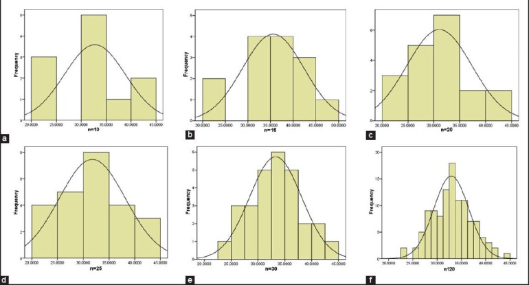
Sample size has a significant effect on sample distribution. It is often observed that small sample size results in non-normal distribution. This is a result of inadequate estimation of the dispersion of the data, and the frequency distribution does not result in a normal curve.[2] To understand the effect of sample size on distribution, let us consider the following research question. What is the shear bond strength of self-etch adhesive to dentin? Figure. 1 shows the distribution of data in different scenarios with increasing sample size. The graph does not conform to the bell curve when the sample size is 10, 15 or 20 [Figure 1a–c]. When the sample size increases to 25 [Figure 1d], the distribution is beginning to conform to the normal curve and becomes normally distributed when sample size is 30 [Figure 1e]. When one rationalizes the normal distribution to the sample size, there is a tendency to assume that the normalcy would be better with very large sample size. However, it can be seen that when the data shows normal distribution at n = 30 [Figure 1e], the distribution remains the same when the sample size is 120 [Figure 1f]. When we look at the mean and SD for different sample sizes [Table 1], it can be noted that the mean varies from 35 to 32 MPa between n = 10 and n = 25, but stabilizes at 33.3 MPa when n = 30. However, the SD is gradually decreasing from 7.57 to 5.04 with an increase in sample size. Hence the shape of the normal distribution is a function of SD. The shape is broader and flatter when SD is high and narrower when SD is low.

Figure 1.

Illustrates frequency distribution of shear bond strength (MPA) values at different sample size (n). (a) n = 10. (b) n = 15. (c) n = 20. (d) n = 25. (e) n = 30. (f) n = 120.

(Note: Sample size of 30 is not always an ideal number that allows normal distribution. It is observed for this data set).

Table 1.

Mean and standard deviation of shear bond strength values (MPa) at different sample sizes.

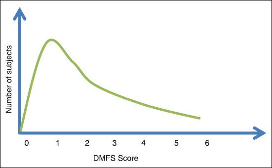
Normal distribution is not the only “ideal” distribution that is to be achieved. Data that do not follow a normal distribution are called non-normal data. In certain cases, normal distribution is not possible especially when large samples size is not possible. In other cases, the distribution can be skewed to the left or right depending on the parameter measure. This is also a type of non-normal data that follows Poisson's distribution independent of the sample size. For example, any data on DMFS would often have skewed distribution to the left. This happens due to the nature of the data set. The best DMFS score is 0 and in a population of school children, the mean DMFS value would be closer to 0 and taper gradually towards the right. [Figure 2] This kind of skewed data is also a true representative of the population.

Figure 2.

Distribution of DMFS scores showing skewed distribution

To know if the data follows normal distribution, we can use tests like Shapiro-Wilk test or Anderson-Darling test or Kolmogonov-Smirnov test to check for normalcy.[3] If the data follows normal distribution, we can use parametric methods for data analysis. When the data does not follow normal distribution, we can transform the data (logarithmic transformations) or use a statistical method that does not consider the distribution for analysis.

Statistical notes:

• The parameters of normal distribution are mean and SD.

• Distribution is a function of SD.

• Sample size plays a role in normal distribution.

• Skewed distribution can also be representative if the population under study.

• Normal distribution of data can be ascertained by certain statistical tests.

REFERENCES

- 1.Krithikadatta J, Valarmathi S. Research Methodology in dentistry: Part II — The relevance of statistics in research. J Conserv Dent. 2012;15:206–213. doi: 10.4103/0972-0707.97937. [DOI] [PMC free article] [PubMed] [Google Scholar]
- 2.Altman D, Bland M. The normal distribution. BMJ 1995. 1995:298. doi: 10.1136/bmj.310.6975.298. [DOI] [PMC free article] [PubMed] [Google Scholar]
- 3.Razali, Nornadiah, Wah, Yap Bee. Power comparisons of Shapiro-Wilk, Kolmogorov-Smirnov, Lilliefors and Anderson-Darling tests. Journal of Statistical Modeling and Analytics. 2011;2:21–33. [Google Scholar]