RNA-Seq Analysis of Gene Expression and Alternative Splicing by Double-Random Priming Strategy

Abstract

Transcriptome analysis by deep sequencing, more commonly known as RNA-seq is, becoming the method of choice for gene discovery and quantitative splicing detection. We published a double-random priming RNA-seq approach capable of generating strand-specific information [Li et al., Proc Natl Acad Sci USA 105:20179–20184, 2008]. Poly(A)⁺ RNA from a treated and an untreated sample were utilized to generate RNA-seq libraries that were sequenced on the Illumina GA1 analyzer. Statistical analysis of approximately ten million sequence reads generated from both control and treated cells suggests that this tag density is sufficient for quantitative analysis of gene expression. We were also able to detect a large fraction of reads corresponding to annotated alternative exons, with a subset of the reads matching known and detecting new splice junctions. In this chapter, we provide a detailed, bench-ready protocol for the double-random priming method and provide user-friendly templates for the curve-fitting model described in the paper to estimate the tag density needed for optimal detection of regulated gene expression and alternative splicing.

1. Introduction

We have devised a procedure based on double-random priming and solid phase selection to produce libraries for high-throughput sequencing on the Illumina Genome Analyzer (1). In order to sequence these libraries, P1 and P2 adapter sequences must be added to the ends of the DNA of interest. In this protocol, double poly(A)-selected RNA is first primed with an oligonucleotide that contains a random octamer and the P1 adapter sequence. This first primer also carries a biotin moiety at the 5′ end, which allows for the capture of extended cDNA product on streptavidin beads. A second random primer linked to the other sequencing primer (P2) adapter sequence is next added to the cDNA bound to the streptavidin-coated magnetic beads. After extensive washes, potential P2 dimers are eliminated and the second random primed products are released from the beads by heat, leaving behind unused P1 primer, P1-extended cDNA, and potential P1 dimers. The released products are PCR amplified, gel purified to enrich for amplicons in the size range of 100–300nt, quantified, and subjected to sequencing (from the P1 primer side) on the Illumina/Solexa flow cell.

This procedure has several advantages compared to previous published protocols. First, it provides strand-specific information, as opposed to other methods that convert RNA to cDNA before primer addition. Second, sequencing a short region right after the first random priming reaction avoids cDNA artifacts resulting from extension of the hairpins formed after the first strand synthesis (2), which may account for artifactual “antisense transcripts” seen in previous large-scale mRNA sequencing and tiling analysis (3,4). Third, the built-in random primer region retains the molecular memory for originally primed products, allowing computational elimination of sequenced reads amplified by PCR, because all PCR products from the same initial amplicon will have identical sequences in the randomized region. This strategy permits the use of PCR amplification without distorting the representation of the transcriptome, a feature critical for quantitative analysis on a limited population of cells.

2. Materials

2.1. Total RNA Extraction Reagents

1. RNAbee (amsbio).

2.2. Double-Random Priming Reagents

1. RT buffer (Invitrogen): First-strand buffer (5×), DTT (0.1 M), RNase inhibitor, Superscript III reverse tran-scriptase, 10 mM dNTPs, and RNAase-free water (Invitrogen Superscript III kit).

2. QIAquick PCR purification kit (Qiagen):

   1. Qiagen PCR purification buffer.

   2. Qiagen purification columns.

   3. Qiagen binding buffer.

   4. Qiagen wash buffer.

   5. Qiagen elution buffer: 10 mM Tris–HCl, pH 8.5.

3. NaOH (0.1 M).

4. 10 mM dNTPs.

5. 130 mM ddNTPs.

6. Adaptor 1: Biotinylated random oligo with Solexa Adaptor P1: (Bio-P1-N(8)) OR biotinylated oligo-dT with Solexa Adaptor P1 (Bio-P1-poly(T)⁺), 50 μM (see ^{Note 3}).

7. Terminal transferase (NEB).

8. 10× Terminal transferase buffer (NEB).

9. EDTA.

10. Beads: Streptavidin-coated magnetic beads (SeraMag beads of Seradyne or Dynal beads).

11. Magnetic stand (Dynal).

12. Adaptor 2: Random oligo-linked Solexa Adaptor P2 (P2-N(8)) (100 μM).

13. PCR buffer: 10× standard Taq DNA polymerase buffer (NEB).

14. Wash buffer: 10 mM Tris-HCl, pH 7.5, 1 mM EDTA, 0.1% Tween-80 or Triton-X 100.

15. Taq DNA polymerase (NEB).

16. Agarose (NuSieve).

17. PicoGreen (Invitrogen).

3. Methods

3.1. Double-Random Priming Method

3.1.1. Reverse Transcription

The bench-ready protocol is described as follows:

1. Add 1 μl of Adaptor 1 (reagent 6) to 10 pg–5 μg of total RNA, 1 μl of dNTP mix, and RNase-free water to 13 μl per reaction.

2. Heat the mixture to 65°C for 5 min and incubate on ice for at least 1 min.

3. Add 4 μl of RT buffer.

4. Incubate at 50°C for 30–60 min.

5. Add deionized water to a total volume of 100 μl and inactivate the reaction by heating at 70°C for 15 min.

6. To remove the free biotin-labeled oligos, add 500 μl of Qiagen PCR purification buffer before transferring the mixture to a Qiagen purification column. Wash the Qiagen column once with the binding buffer and twice with the wash buffer. Elute with 50 μl of Qiagen elution buffer to a clean tube.

3.1.2. First Primer Blocking and Random Primer Extension Reaction

1. Transfer the eluate to PCR tubes. Add 15 μl of terminal transferase buffer, 3 μl of ddNTP mix and DI water to make up the volume to 150 μl. Add 2 μl of terminal transferase enzyme. Incubate at 37°C for 1 h (see ^{Note 1}).

2. Add 20 mM of EDTA.

3. Add 5 μl of beads and incubate the mixture at room temperature for 20 min.

   Collect the beads with a magnetic stand and discard the supernatant (see ^{Note 4}).

   Remove the tubes containing beads from the magnetic stand. Wash the beads with 100 μl of NaOH solution by drawing beads to oneside of the tube then the other with the magnetic stand (see ^{Note 4}). Incubate for 5 min at room temperature.

4. Collect the beads with the magnetic stand and wash with DI water twice, removing the tubes from the magnetic stand between washes to wash completely.

5. Off the magnetic stand, add 1 μl of Adaptor 2 to the beads, 5 μl of PCR buffer, 1 μl of dNTPs, add DI water to make up the volume to 49 μl. Add 1 μl of Taq DNA polymerase (5 U).

6. Incubate the tubes at 25°C for 1 h. Heat to 72°C for 30 s and then raise the temperature to 75°C for 5 min. Add 10 mM of EDTA to to stop the polymerization reaction.

7. Collect the beads and wash twice with 150 μl of wash buffer, removing the tubes from magnetic stand during washes.

8. On the stand, add 20 μl of water and heat for 5 min at 95°C. Collect the extended DNA in the supernatant.

9. Amplify the extended DNA with PCR using Solexa Adaptors 1 and 2 as primers (without poly(T)⁺ or N(8)).

10. Run the library on an agarose gel and excise the band corresponding to 75–125 nt. Gel extract the band to elute DNA library.

11. Quantify DNA using PicoGreen or quantitative PCR prior to sequencing. A typical sequencing run uses 10–20 ng of DNA.

3.2. Transcript Databases for Gene Expression and Alternative Splicing Detection

In order to utilize RNA-seq reads to measure gene expression quantitatively, it is imperative to first define our concept of genes. To that end, we have developed detailed annotations of gene structures based on publicly available annotations downloaded from the University of California, Santa Cruz (UCSC) (5). We have also generated alignable sequence databases that can be used with data generated from high-throughput sequencing and for the purpose of aligning sequencing reads to spliced mRNA transcripts. Basic notes on the acquisition and processing of data such as these are outlined here. Please review our previously published work for more detailed information (6).

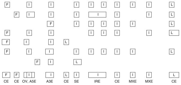
3.2.1. Building an Aggregate Gene Model (Fig. 1)

Fig. 1.

Cartoon depicting construction of an aggregate gene model. Exons are depicted as boxes labeled as internal (I), first (F), or last (L). Region classifications are listed at the bottom of the schematic. Classifications of splicing were defined as follows: overlap (OV), skipped exons (SE), alternative 5′/3′ exons (A5E/3E), constitutive exons (CE), mutually skipped exons (MXE), and intron retentions (IRE).

Genome sequences of human (hg17) and annotation for protein-coding genes were obtained from the UCSC. The lists of known human genes (knownGene containing 43,401 entries) and knownisoforms (knownIsoforms containing 43,286 entries in 21,397 unique isoform clusters) with annotated exon alignments to human hg17 genomic sequence were processed as follows. Knowngenes that were mapped to >1 isoform clusters were discarded. All mRNAs aligned to the human genome that were >300 bases long were clustered together with the knownisoforms. For the purposes of measuring differential gene expression, all genes were considered. For the purposes of inferring alternative splicing, genes containing <3 exons were not considered. Exons with canonical splice signals (GT-AG, AT-AC, and GC-AG) were retained, resulting in a total of 213,736 exons. Of these, 92% of all exons were constitutive exons, 7% had evidence of exon skipping, 1% of exons were mutually exclusive alternative events, 3% of exons had alternative 3′ splice sites, and 2% exons had alternative 5′ splice sites (Fig. 1). A total of 2.7 million spliced ESTs were mapped onto the 17,478 high-quality gene clusters to identify alternative splicing. To eliminate redundancies in this analysis, final annotated gene regions were clustered together so that any overlapping portion of these databases was defined by a single genomic position.

3.2.2. Building an Exon-Junction Database

Exons with canonical splice signals (GT-AG, AT-AC, and GC-AG) were used to create an exon-junction database (EJDB). For each protein-coding gene, the 35 bases at the 3′ end of each exon were concatenated with the 35 bases at the 5′ end of the downstream exon. This was repeated, joining every exon of a gene to every exon downstream. This approach produced 1,929,065 theoretical splicing junctions. An equal number of “impossible” junctions were generated by joining the 35-base exon-junction sequences in reverse order.

3.3. Metrics for Differential Gene Expression

3.3.1. Alignment

MosaikAligner (7), using a maximum of 2 mismatches over 95% alignment of the tag (34nt) and a hash size of 15, was used to align reads to the human genome (hg17). However, since the publication of this work, several new alignment algorithms have been made available that offer other options for this step (such as QPalma (8) Bowtie (9) or RazerS (10)). To determine the number of reads contained within protein-coding genes, promoter, and intergenic regions, we arbitrarily defined promoter regions as regions 3-kb upstream of the transcriptional start site of the gene, and intergenic regions as unannotated regions in the genome.

Alignments to our EJDB were also done using the same alignment algorithm and mapping requirements, with the added requirement that reads map at least 4 nt across the exon–exon junction.

3.3.2. Evaluation of Differential Gene Expression

Differentially expressed transcripts were identified by enumerating the number of reads that mapped within the spliced mRNA transcript in untreated and hormone-treated cells, using the total number of reads mapped to exons in each condition as a basis for determining significance by the χ² statistic.

The χ² statistic was calculated for genes with ≥ 5 reads in each experimental condition, and the value of the χ² statistic was computed using a 2 × 2 square with the reads within a particular gene in both conditions on the top row and the reads not within that gene in both conditions on the bottom row.

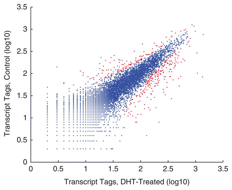
After the number of reads mapped in each condition and the statistical significance are determined, each gene can be plotted as a scatter plot as in Fig. 2 for visualization purposes.

Fig. 2.

Digital analysis of androgen-regulated gene expression in LNCaP cells. Scatter plot of gene expression in mock-treated and DHT-induced cells. Differential expressed genes were (in light gray) based on χ² analysis (P < 0.01).

3.3.3. Detection of Alternative Splicing

Alternative splicing was detected by using reads mapped across exon junctions. We were able to detect both annotated and novel splice junctions. The type of exon–exon junction (i.e., constitutive or alternative) was determined based on our aggregate gene model (see above). False-discovery rate (FDR) was assessed by mapping reads to a set of “impossible” junctions that were created by reversing the order of exons in the EJDB (e.g., if exons 1 and 2 of a particular gene that are in the EJDB are joined 1 → 2, the impossible version of this would be the same exons joined in the reverse order, 2 → 1).

3.4. Power Curve Analysis

To establish the depth of sequencing required to examine several transcriptome features, we devised a method to predict not only the number of reads required to analyze a particular feature, but also the number of features observable at that sequencing depth. Reads were randomly sampled into subsets representing 10, 20%, etc., of the total number of sequence reads available using custom Perl scripts. These were aligned as described above and the number of features detected was assessed. To determine the number of sequence reads required to reach a user-defined threshold for saturation, the percentage change in discovering additional features was determined as follows:

$$\begin{array}{l}T(n)=sn,\\ C(n)=\left(\frac{F(n)-F(n-1)}{F(n-1)}\right),\end{array}$$

where T(n) is the number of reads, s is the sampling size (in our case, two million reads), n is a constant multiplier, C(n) is the empirical change in number of features detected, and F(n) is the number of empirical features detected at n. A scatter plot of C(n) to T(n) was fitted with a power curve of the form c(n) = a×T (n)^b and an exponential curve of the form c(n) = ae^bT(n), where c (n) is the change estimated by the curve fitting.

The equation that had the best fit, indicated by r², was used to extrapolate the tag density required to achieve a defined change in the number of features detected. The number of estimated features was calculated by

$$f(n)=\sum _{t=m}^{n}f(i-1)+f(i-1)\times c(i),$$

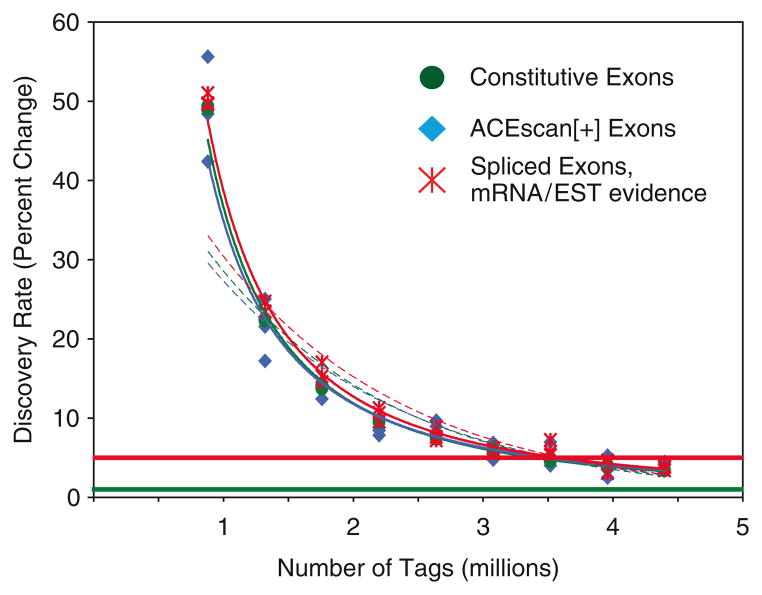
where m is user defined (in our case, m = 6). This will compute the predicted number of features observable based on observed change in feature detection, extrapolated from an area in the middle of the curve. Fig. 3 depicts one such fitted curve.

Fig. 3.

Curve fitting the change in the number of exons and splice junctions detected against increasing tag densities. Dashed line indicates exponential curve; solid line indicates power curve. Decline in the rate of identifying additional exons as a function of increasing tag density.

These calculations can be done easily using the “Data Analysis” ToolPak for Microsoft Excel. An example worksheet that calculates features using data from three independent samplings (labeled X, Y, and Z) can be downloaded from http://yeolab.ucsd.edu/yeolab/Papers_files/EXAMPLE.xls

References

- 1.Li H, Lovci MT, Kwon YS, Rosenfeld MG, Fu XD, Yeo GW. Determination of tag density required for digital transcriptome analysis: application to an androgen-sensitive prostate cancer model. Proc Natl Acad Sci USA. 2008;105:20179–20184. doi: 10.1073/pnas.0807121105. [DOI] [PMC free article] [PubMed] [Google Scholar]
- 2.Perocchi F, Xu Z, Clauder-Munster S, Steinmetz LM. Antisense artifacts in transcriptome microarray experiments are resolved by actinomycin D. Nucleic Acids Res. 2007;35:e128. doi: 10.1093/nar/gkm683. [DOI] [PMC free article] [PubMed] [Google Scholar]
- 3.Carninci P, Kasukawa T, Katayama S, et al. The transcriptional landscape of the mammalian genome. Science. 2005;309:1559–1563. doi: 10.1126/science.1112014. [DOI] [PubMed] [Google Scholar]
- 4.Cheng J, Kapranov P, Drenkow J, Dike S, Brubaker S, Patel S, Long J, Stern D, Tammana H, Helt G, Sementchenko V, Piccolboni A, Bekiranov S, Bailey DK, Ganesh M, Ghosh S, Bell I, Gerhard DS, Gingeras TR. Transcriptional maps of 10 human chromosomes at 5-nucleotide resolution. Science. 2005;308:1149–1154. doi: 10.1126/science.1108625. [DOI] [PubMed] [Google Scholar]
- 5.Karolchik D, Baertsch R, Diekhans M, Furey TS, Hinrichs A, Lu YT, Roskin KM, Schwartz M, Sugnet CW, Thomas DJ, Weber RJ, Haussler D, Kent WJ. The UCSC genome browser database. Nucleic Acids Res. 2003;31:51–54. doi: 10.1093/nar/gkg129. [DOI] [PMC free article] [PubMed] [Google Scholar]
- 6.Yeo GW, Van Nostrand EL, Liang TY. Discovery and analysis of evolutionarily conserved intronic splicing regulatory elements. PLoS Genet. 2007;3:e85. doi: 10.1371/journal.pgen.0030085. [DOI] [PMC free article] [PubMed] [Google Scholar]
- 7.Hillier LW, Marth GT, Quinlan AR, et al. Whole-genome sequencing and variant discovery in C. elegans. Nat Meth. 2008;5:183–188. doi: 10.1038/nmeth.1179. [DOI] [PubMed] [Google Scholar]
- 8.De Bona F, Ossowski S, Schneeberger K, Ratsch G. Optimal spliced alignments of short sequence reads. Bioinformatics. 2008;24:i174–i180. doi: 10.1093/bioinformatics/btn300. [DOI] [PubMed] [Google Scholar]
- 9.Langmead B, Trapnell C, Pop M, Salzberg SL. Ultrafast and memory-efficient alignment of short DNA sequences to the human genome. Genome Biol. 2009;10:R25. doi: 10.1186/gb-2009-10-3-r25. [DOI] [PMC free article] [PubMed] [Google Scholar]
- 10.Weese D, Emde AK, Rausch T, Doring A, Reinert K. RazerS–fast read mapping with sensitivity control. Genome Res. 2009;19:1646–1654. doi: 10.1101/gr.088823.108. [DOI] [PMC free article] [PubMed] [Google Scholar]