HOW DOES COST MATTER IN HEALTH-CARE DISCRETE-CHOICE EXPERIMENTS?

SUMMARY

Willingness-to-pay (WTP) estimates derived from discrete-choice experiments (DCEs) generally assume that the marginal utility of income is constant. This assumption is consistent with theoretical expectations when costs are a small fraction of total income. We analyze the results of five DCEs that allow direct tests of this assumption. Tests indicate that marginal utility often violates theoretical expectations. We suggest that this result is an artifact of a cognitive heuristic that recodes cost levels from a numerical scale to qualitative categories. Instead of evaluating nominal costs in the context of a budget constraint, subjects may recode costs into categories such as ‘low’, ‘medium’, and ‘high’ and choose as if the differences between categories were equal. This simplifies the choice task, but undermines the validity of WTP estimates as welfare measures. Recoding may be a common heuristic in healthcare applications when insurance coverage distorts subjects’ perception of the nominal costs presented in the DCE instrument. Recoding may also distort estimates of marginal rates of substitution for other attributes with numeric levels. Incorporating ‘cheap talk’ or graphic representation of attribute levels may encourage subjects to be more attentive to absolute attribute levels.

1. INTRODUCTION

Empirical studies using choice-format conjoint surveys or discrete-choice experiments (DCEs) to estimate willingness-to-pay (WTP) generally assume that the marginal utility of income is constant (Just et al., 1982; McCloskey, 1982). This is equally the case in studies of health-care choices. (See, e.g. Ryan, 2004; Hanley et al., 2003; Maddala et al., 2003; Olsen and Smith, 2001; Bryan et al., 2000; Tesler and Zweifel, 2002.) However, constant MUY may be violated in some instances, raising legitimate concerns about whether WTP estimates are valid welfare measures.

Statistically, MUY implies a linear cost specification in health-care DCE models. Most health care studies follow the convention of estimating WTP by dividing the estimated utility difference between an intervention or outcome and a reference condition by a constant marginal utility of income, indicated by the absolute value of the cost-attribute coefficient.¹ To interpret the resulting rescaled utility difference as a utility-theoretic measure of WTP, it is also necessary to assume that subjects accept indicated cost levels as personal, income-constrained, out-of-pocket expenses required to obtain the improved outcome.

Yet, there is little empirical evidence as to how DCE subjects evaluate health-care cost information. Unlike preference studies in other areas, health care often is partly or fully insured. Study subjects, unaccustomed to evaluating costs as high as those presented in the DCE trade-off tasks, may employ cognitive strategies to decrease the considerable mental effort these tasks require (Payne et al., 1993). DCE subjects may ignore costs altogether in evaluating trade-offs, or lower indicated costs because they are accustomed to paying only a fraction of actual costs. In other cases, cost levels may be recoded to, e.g. ‘low,’ ‘medium,’ and ‘high’ categories. Recoding may be a strategy for simplifying evaluations of a relatively unfamiliar but important attribute. Measurement error or bias may result because of differences between the cost levels used in estimation and the cost levels subjects use in their evaluations of trade-off tasks.

This study assesses the consequences of estimating WTP, assuming a linear opportunity–cost specification when actual preferences may be inconsistent with that specification. For each of the five DCE studies (colorectal cancer screening (CRC), HIV testing, insulin devices, a public-health intervention to reduce the risk of developing diabetes, and insulin therapies for Type 2 diabetes), we explore the consequences of two strategies: (1) linearizing preferences to fit conventional assumptions, and (2) taking subjects’ stated preferences at face value and calculating welfare effects using alternative nonlinear MUY estimates.

2. METHODS

2.1. Data

Table I presents five datasets. Each survey’s design was similar, and included demographic and health history questions, definitions of attributes and levels, and 8–12 choice format trade-off questions. We employed a D-optimal algorithm to construct a near-optimal experimental design (Huber and Zwerina, 1996; Kanninen, 2002; Zwerina et al., 1996). While the range of costs varies across studies, all the ranges overlap at 11 or more points. Figure 1 presents an example trade-off question for insulin in Type-2 diabetes.

Table I.

Description of the five US DCE studies

Patient study	Cost levels (US dollars)	Number of subjects	Number of alternatives	Number of trade-off questions
Colorectal Cancer (CRC) Screening Tests	25, 100, 500, 1000	1087	2	12
HIV Testing Programs	0, 10, 50, 100	323	2	10
Diabetes Prevention Programs	0, 25, 50, 100, 200	703	3*	9
Insulin Devices	100, 175, 225, 300	392	2	8
Insulin Therapies	50, 100, 150, 200	737	3*	10

^*Third alternative was a status-quo reference condition or opt-out alternative.

Figure 1.

Example choice question

2.2. Analysis

Step 1

For each dataset we estimated fixed-effect, conditional logit models with the following random-utility specification:

$$\begin{array}{l}{V}_k^i=U_k^i+{\epsilon }_k^i,\hfill \\ U_k^i=\sum {\alpha }_j^i{X}_{jk}^i+f_i(C_k^i)\hfill \end{array}i=1,\dots ,6$$ (1)

where for dataset i, choice k, $V_k^i$ is the random utility, $U_k^i$ and ${\epsilon }_k^i$ are the determinate and stochastic expressions, $X_{jk}^i$ is attribute level j, ${\alpha }_j^i$ is the corresponding part-worth coefficient, and $f_i(C_k^i)$ is 1 of 3 specifications: linear, log, or categorical.

$$f_i(C_k^i)=\{\begin{array}{ll}{\beta }_{\text{lin}}^i·C_k^i\hfill & \text{linear}\hfill \\ {\beta }_{log}^i·ln(C_k^i)\hfill & log\hfill \\ {\beta }_m^i·C_{\text{km}}^i\hfill & \text{categorical},m=1,\dots ,\text{number}\text{of}\text{cost}\text{levels}\hfill \end{array}$$ (2)

All categorical variables were effects-coded (Hensher et al., 2005). As indicated, linear specification is the conventional estimation strategy. Log transformations are commonly used to model continuous, nonlinear variables. Estimating cost as a categorical variable imposes no functional-form restrictions on preferences.

Step 2

For each dataset, we calculated a change in utility (ΔUⁱ) that yields a WTP of $100 using the linear-cost model.

$$\begin{array}{l}{\text{WTP}}^i=100=\frac{\mathrm{\Delta }{U}^i}{-{\beta }_{\text{lin}}^i}\\ \mathrm{\Delta }{U}^i=-100·{\beta }_{\text{lin}}^{i}i=1,\dots ,6\end{array}$$ (3)

This calculation assumes constant $\text{MUY}=-{\beta }_{\text{lin}}^i$, but allows the linear MUY estimate to vary across datasets.

Step 3

Using the same ΔUⁱ for each study, we calculated WTPⁱ using the log-cost model evaluated at the mean cost C̄ⁱ as follows:

$${\text{WTP}}_{log}^i=\frac{\mathrm{\Delta }{U}^i}{-{\beta }_{log}^i/{\overline{C}}^i}$$

Step 4

Again, using the same ΔU, we calculated WTPⁱ using the categorical cost levels in three different ways:

• Lowest–Highest:

  $${\text{WTP}}_{\text{low}-\text{high}}^i=\frac{\mathrm{\Delta }{U}^i}{{\beta }_{\text{low}-\text{high}}^i}={\beta }_{\text{low}-\text{high}}^i=\frac{{\beta }_{\text{lowest}}^i-{\beta }_{\text{highest}}^i}{C_{\text{highest}}^i-C_{\text{lowest}}^{ii}},$$

  where β_lowest corresponds to the lowest cost category and β_highest corresponds to the highest cost category.

• Mean of categorical slopes:

  $${\text{WTP}}_{\text{mean}}^i=\frac{\mathrm{\Delta }{U}^i}{{\beta }_{\text{mean}}^i},{\beta }_{\text{mean}}^i=\frac{1}{n-1}·\sum _{m=1}^{n-1}\frac{{\beta }_m^i-{\beta }_{m+1}^i}{C_m^i-C_{m+1}^i},$$

  where n is the number of cost levels.

• Piecewise linear:

  $${\text{WTP}}_{\text{piece}}=C_m^i+\frac{\mathrm{\Delta }{U}^i+{\beta }_m^i}{C_{m+1}^i-C_m^i}·(C_{m+1}^i-C_m^i),$$

  where $m={max}_m({\beta }_m^i-{\beta }_1^i<\mathrm{\Delta }{U}^i)$.

Step 5

We checked each dataset for cost recoding. If MUY is constant, the scatter plot of predicted utility against nominal cost should be linear. If cost differences increase for higher cost levels, the plot of utility against categorical cost should be concave. However, if the plot against categorical cost is approximately linear, the utility difference for small cost differences is the same as for large cost differences, suggesting that subjects have recoded the nominal costs as ‘low,’ ‘medium,’ and ‘high’ with similar utility differences between recoded categories (see Figure 2). The categorical coefficients may decrease with the cost level, and may be significantly different from one another, but their values are inconsistent with the actual differences in nominal cost levels. A linear cost specification generally will yield a negative and statistically significant cost coefficient in this case. Thus, researchers are likely to interpret this result as being consistent with theoretical expectations.

Figure 2.

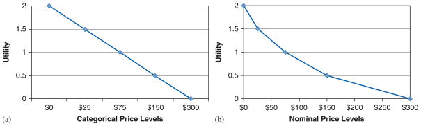
Cost recoding examples. (a) Constant marginal utility of price categories and (b) Non-constant marginal utility of nominal prices

3. RESULTS

Figure 3 compares the WTP estimate from the linear model of the diabetes-prevention data to 22 alternative specifications: a log model with the WTP evaluated at the mean cost, and a piecewise linear model. (Numeric estimates from all 44 models appear in the Diabetes Prevention row of Table II.)

Figure 3.

Diabetes prevention recoding results

Table II.

WTP estimated by different methods when linear price produces $100 WTP (95% confidence intervals in parentheses)

Dataset	Price/cost levels	Linear price (WTP 5$100)	Log price	Lowest–highest	Mean of piecewise slopes	Piecewise linear
CRC screening	25/100/500/1000	100	170 (156–187)	104 (96–114)	121 (87–195)	143 (71–218)
HIV testing	0/10/50/100	100	224 (199–255)	57 (52–64)	58 (52–64)	64 (59–69)
Insulin devices	100/175/225/300	100	133 (105–182)	101 (82–131)	100 (81–132)	101 (81–195)
Diabetes prevention	0/25/50/100/200	100	79 (73–85)	113 (103–125)	84 (77–92)	54 (60–78)
Insulin therapies	50/100/150/200	100	137 (130–146)	101 (95–108)	101 (95–108)	111 (104–117

Applying Equation (1), the utility difference in Figure 3 corresponding to a WTP of $100 is dU₁₀₀=1.2 for the linear model. This utility difference corresponds to a WTP of about $79 for the log model (with the rate of change evaluated at the mean cost), and $54 for the piecewise-linear model.

Table II presents the results of our analysis for all five datasets. The first two columns list the dataset and the cost levels. The remaining five columns show the WTP estimates using each of the alternate methods.

• Log Cost: Differences in WTP for the log cost model are strongly influenced by differences in cost ranges among surveys.

• Lowest/Highest: In general, this method created very similar WTP estimates as the linear cost. There was only 1 case (HIV) where the lowest–highest cost was much lower than the linear cost (and see Figure 2).

• Mean of Piecewise Slopes: In general, this method also produced similar WTP estimates as the linear cost. There was only one case (HIV) where the mean slope WTP estimate was much lower than the linear cost.

• Piecewise Linear: The estimated WTP was much lower than the linear model for diabetes prevention and HIV, nearly identical for insulin devices, somewhat higher for insulin therapies, and much higher for CRC.

The spacing and range of cost levels offered are possible sources of discrepancies among the models. In the case of the largest observed difference, the CRC testing study, categorical estimates for the $25, and $100 cost levels are nearly identical. This causes the categorical estimates to lie to the right of the linear model and the slope of the linear model to be steeper than the average piecewise slope. It is likely that the $500 and $1000 cost levels made the difference between $25 and $100 appear small to subjects.

The first two categorical estimates for the HIV testing study were also virtually identical. Here, the range is only $100, but the difference between the $0 and the $10 cost for a test apparently was perceived as negligible. As in the CRC case, the slope of the linear model is steeper than the average piecewise slope.

While the cost levels offered in the two testing studies seemed reasonable, they appear to have unintended cognitive consequences. Apart from the first two levels, the utility gradient with respect to cost is consistent with constant MUY. Choosing two levels close to one another apparently resulted in spurious estimates. The spacing and ranges of the cost attribute in the other studies were less likely to trigger this pattern of responses. The effect of a small utility change between the first two categories increases the piece-wise linear WTP calculation in the categorical model.

The diabetes-prevention study is the only case where the linear model overstates WTP based on observed trade-off preferences – an apparent case of cost recoding (Figure 3). The utility plot against categorical cost should be linear if marginal utility is constant. A plot against unequally spaced cost categories should consequently be concave. If the scatter plot is convex and the category plot is linear, then the utility differences between categories are equal, regardless of the actual cost intervals. The implication is that responses would have been the same regardless of the actual cost values.

4. DISCUSSION

This paper presents alternative ways of estimating marginal utility of income when cost recoding exists. We caution researchers that the best method for estimating the marginal utility of income is situationspecific and should be tested for fit in particular cases. Nonetheless, a common criticism of statedpreference studies, including DCE studies, is that they rely on evaluations of hypothetical alternatives. Such evaluations do not have the same clinical, financial, and emotional consequences as real healthcare decisions. It is important to assess the validity of DCEs by checking response consistency and conformity to utility-theoretic requirements. However, we are unaware of any study that has tested the marginal utility of income assumption that is crucial to calculating WTP.

Recoding cost levels has significant welfare-economic implications. With recoding, WTP estimates become an artifact of the labels researchers attach to the cost levels, not subjects’ measured trade-off preferences. Utilizing the recoding heuristic in stated-preference studies could invalidate welfare estimates for revealed preference studies, as well.

Researchers agree that it is important to motivate the cost attribute carefully. Investigators in other areas (e.g. environmental economics) have proposed including ‘cheap talk’ text to encourage more attentive evaluation of costs – generally in the context of contingent-valuation studies rather than DCEs (Cummings and Taylor, 1999; List, 2001; Aadland and Caplan, 2006). Cheap-talk strategies co-opt subjects into becoming part of the research team by alerting them to common errors that ‘other people’ often make in answering stated-preference questions, which degrade the integrity of the study (Murphy et al., 2005).

The success of this approach, principally in contingent-valuation studies, has been mixed. If recoding is a heuristic similarly linked to hypothetical bias, then a cheap-talk text could improve DCE subjects’ attention to nominal cost levels. The sole study applying cheap talk to a DCE survey investigated its effect on a cost attribute (Ö zdemir et al., 2009). Ö zdemir et al. found that the cost function for the cheap-talk subsample was linear, while the cost function for the control subsample was not. Cheap talk affected the coefficient on the cost attribute, as well as preferences for other attributes.

Our results suggest that one cannot assume that the cost gradient is continuous and linear. The minimal effort required to apply the categorical model rejected linearity in two cases and yielded important insights, including possible evidence of recoding. Researchers should check for possible violations of the constant marginal utility of income assumption. If cost estimates are inconsistent with conventional assumptions, researchers should determine how to model this behavior, assess what consequences these anomalies may have for welfare calculations, and consider ways to encourage theoretic responses in future surveys.

As a test of a recoding hypothesis, this study has several limitations. First, none of the studies was explicitly designed for that purpose. It is not possible to detect recoding when cost levels are spaced equally. Indeed, we cannot rule out the possibility of recoding in the three studies that yielded approximately constant MUY, all of which had constant or near-constant differences in adjacent cost levels. In those cases, our test is weaker than in studies where differences are more marked. We also cannot unambiguously rule out competing hypotheses involving cognitive responses other than recoding. We also did not look at split sample analyses for each study to determine whether there were differences in recoding among groups. Finally, variations among the studies as to commodity evaluated, information provided about attributes, numbers of attributes and levels involved, and layout of the trade-off task may be confounded with any anomalies observed in estimates of the cost response.

Future research should focus on identifying best-practice methods for incorporating cost in DCEs. A controlled experiment holding all variables constant except for survey features related specifically to the cost attribute, including controlled variations in motivation for costs, budget reminder, cheap talk, and the range and spacing of the cost levels would be informative. Understanding DCE subjects’ cognitive responses to trade-off tasks are important for obtaining results that can be interpreted as valid approximations of welfare changes.

References

- Aadland D, Caplan AJ. Cheap talk reconsidered: new evidence from CVM. Journal of Economic Behavior & Organization. 2006;60:562–578. [Google Scholar]
- Bryan S, Gold L, Sheldon R, Buxton M. Preference measurement using conjoint methods: an empirical investigation of reliability. Health Economics. 2000;9(5):385–395. doi: 10.1002/1099-1050(200007)9:5<385::aid-hec533>3.0.co;2-w. [DOI] [PubMed] [Google Scholar]
- Cummings RG, Taylor LO. Unbiased value estimates for environmental goods: a cheap talk design for the contingent valuation method. American Economic Review. 1999;89(3):649–666. [Google Scholar]
- Hanley N, Ryan M, Wright R. Estimating the monetary value of health care: lessons from environmental economics. Health Economics. 2003;12(1):3–16. doi: 10.1002/hec.763. [DOI] [PubMed] [Google Scholar]
- Hensher DA, Rose JM, Greene WH. Applied Choice Analysis: A Primer. Cambridge University Press; Cambridge, United Kingdom: 2005. [Google Scholar]
- Huber J, Zwerina K. The importance of utility balance in efficient choice designs. Journal of Marketing Research. 1996;33:307–317. [Google Scholar]
- Just RE, Hueth DL, Schmitz A. Applied Welfare Economics and Public Policy. Prentice-Hall, Inc; Englewood Cliffs, NJ: 1982. [Google Scholar]
- Kanninen B. Optimal design for multinomial choice experiments. Journal of Marketing Research. 2002;39:214–227. [Google Scholar]
- Lancsar E, Savage E. Deriving welfare measures from discrete choice experiments: inconsistency between current methods and random utility and welfare theory. Health Economics. 2004;13:901–907. doi: 10.1002/hec.870. [DOI] [PubMed] [Google Scholar]
- List JA. Do explicit warnings eliminate the hypothetical bias in elicitation procedures? Evidence from field auction experiments. American Economic Review. 2001;91(5):1498–1507. [Google Scholar]
- Maddala T, Phillips KA, Johnson FR. An experiment on simplifying conjoint analysis designs for measuring preferences. Health Economics. 2003;12(12):1037–1047. doi: 10.1002/hec.798. [DOI] [PubMed] [Google Scholar]
- McCloskey DN. The Applied Theory of Price. 2. Macmillan Publishing Company; New York: 1982. [Google Scholar]
- Murphy JJ, Stevens T, Weatherhead D. Is cheap talk effective at eliminating hypothetical bias in a provision point mechanism? Environmental and Resource Economics. 2005;30(3):327–343. [Google Scholar]
- Olsen JA, Smith RD. Theory versus practice: a review of ‘willingness to pay’ in health and health care. Health Economics. 2001;10(1):39–52. doi: 10.1002/1099-1050(200101)10:1<39::aid-hec563>3.0.co;2-e. [DOI] [PubMed] [Google Scholar]
- Özdemir S, Johnson FR, Hauber AB. Hypothetical bias, cheap talk, and stated willingness to pay for health care. Journal of Health Economics. 2009;28(4):894–901. doi: 10.1016/j.jhealeco.2009.04.004. [DOI] [PubMed] [Google Scholar]
- Payne JW, Bettman JR, Johnson EJ. The Adaptive Decision Maker. Cambridge University Press; New York, NY: 1993. [Google Scholar]
- Ryan M. Deriving welfare measures in discrete choice experiments: a comment to Lancsar and Savage (1) Health Economics. 2004a;13:909–912. doi: 10.1002/hec.869. [DOI] [PubMed] [Google Scholar]
- Ryan M. A comparison of stated preference methods for estimating monetary values. Health Economics. 2004b;13(3):291–296. doi: 10.1002/hec.818. [DOI] [PubMed] [Google Scholar]
- Santos Silva J. Deriving welfare measures in discrete choice experiments: a comment to Lancsar and Savage (2) Health Economics. 2004;13:913–918. doi: 10.1002/hec.874. [DOI] [PubMed] [Google Scholar]
- Tesler H, Zweifel P. Measuring willingness/to/pay for risk reduction: an application of conjoint analysis. Health Economics. 2002;11(2):129–139. doi: 10.1002/hec.653. [DOI] [PubMed] [Google Scholar]
- Zwerina K, Huber J, Kuhfeld W. A General Method for Constructing Efficient Choice Designs. Fuqua School of Business, Duke University; Durham: 1996. [Google Scholar]