

Abstract
The three-dimensional structures of the extended T4 phage tail and polysheath, an aberrant form of the contracted tail sheath, have both been reconstructed from electron micrographs. The reconstructed map of the extended structure is at a somewhat higher resolution (~20 Å) than an earlier reconstruction, allowing tentative boundaries to be drawn between the individual protein subunits in the tail sheath. This improvement has been achieved by testing the degree of correlation between data from different images as part of the selection procedure and averaging the most highly correlated sets of data. Details of the correlation are given in the Appendix. The resolution of the map of the contracted structure is lower than that of the extended tail, in spite of a similar averaging of several images, because of the higher degree of distortion in this structure. Nevertheless, it has been possible, to some extent, to trace the changes in conformation of the subunit during contraction.
1. Introduction
The extended tail of T4 bacteriophage was the first structure to be investigated by the technique of reconstructing three-dimensional images from electron micrographs (DeRosier & Klug, 1968). As the subject has helical symmetry, each image of an extended tail provided enough, data for a complete three-dimensional reconstruction to a limited resolution. Since that time, the reconstruction technique has been applied, not only to a number of other helical structures, but also to spherical viruses with icosahedral symmetry (Crowther et al., 1970; Crowther, 1971), which require that data from different images be scaled together and combined. With increasing complexity in the type of helical structures being studied, methods of combining different images of helical particles have also been developed. Details of the procedures that have been used for finding the relative orientations of different specimens and selecting the “best” images are given in the Appendix. The effect seems to be to average out a significant part of the background noise in the micrographs, allowing a somewhat greater resolution to be achieved in the final density map. The methods described have already been successfully applied to muscle “thin filaments” (Spudich et al., 1972; Wakabayashi et al., 1975), to haemocyanin polymers (Mellema & Klug, 1972), to structures of the tobacco mosaic virus family (Unwin & Klug, 1974; Sperling et al., 1975) and to flagellar microtubules (Amos & Klug, 1974). This paper describes their application to the extended phage tail (Plate I(a)), whose structure has been solved to a higher degree of resolution than before, and to both the contracted tail (Plate I(c)) and the related structure known as polysheath (Plate I(e)), neither of whose three-dimensional structure has been reconstructed before.
Plate I.

Electron microscope images of T4 bacteriophage tail structures, negatively stained with uranyl acctate, and optical diffraction patterns obtained from them.
(a) An extended tail (Magnification 100,000×).
(b) Optical diffraction pattern of (a). The layer lines are numbered according to the selection rule l = −2n + 7m, where n may only have values that are multiples of six (DeRosier & Klug, 1968). The seventh layer line arises from the 41 Å spacing of the stacked rings of subunits in the extended tail. Layer lines out to l = 14 (20 Å) can be identified in the computed Fourier transform although the signal to noise ratio is very low. In the optical transform shown here the 12th layer line (24 Å) is the last that can be detected (best seen in the lower half of the pattern).
(c) A contracted tail showing the core pushed out through the baseplate. Magnification 100,000×.
(d) Optical diffraction pattern of (c). The selection rule is now l = n + 11m (Moody, 1967a). The fifth layer line corresponds to a spacing of 38 Å. No layer lines beyond the sixth can be identified in either the optical or computed transforms.
(e) A length of T4 polysheath. The strong transverse lines are stain-filled grooves between adjacent “short pitch” (0,1) helices (Fig. 1). Magnification 100.000×.
(f) Optical diffraction pattern of (e), which indexes in the same way as the contracted tail pattern (Moody, 1967a). Layer lines beyond l = 6 could not be identified with certainty.
(g) to (j) End-on views of contracted tails, used to determine the radial density distribution of contracted sheath, as shown in Fig. 4(c) ((g) = A, (h) = B, (i) = C, (j) = D).
The tail of the T-even bacteriophages consists of a narrow tubular core, about 90 Å in diameter (Moody, 1971b) surrounded by a sheath with an outer diameter of about 240 Å, as shown in Plate I(a). The core and sheath are each thought to be composed of a single protein species (King & Mykolajewycz, 1973; Dickson, 1974), the products of gene 19 (Mr ~ 20,000) in the case of the core, and of gene 18 (Mt ~ 80,000) in the case of the sheath. At one end of the tail is a complex baseplate constructed of at least 12 protein species, while at the other end a collar connects the tail to the DNA-filled capsid. DNA is injected into the host bacterium by means of a contraction of the tail-sheath, which pushes the rigid tail-tube through the cell wall. Plate I(c) shows a bacteriophage after contraction. According to the measurements of Bayer & Remsen (1970) on freeze-etched T2 particles, the change in outer diameter of the sheath during contraction is from 236 Å to 344 Å. However, they found that in negative stain, whereas the extended sheath shrinks radially only by about 10 Å, the contracted sheath appears to shrink radially to a diameter of 270 Å. Their pictures suggest that the shrinkage caused by the negative stain in the axial direction is small in the case of both structures. Radial shrinkage is common for negatively stained particles, but does not necessarily damage the structure at the level of resolution required to distinguish individual subunits. For example, the diameter of tomato bushy stunt virus particles was found to have shrunk by at least 10% (Crowther et al., 1970); nevertheless, the icosahedral symmetry of isometrically shrunk particles was found to be preserved to about 20 Å resolution.
The process of contraction has been studied extensively by Moody (1967a,b, 1971a,b,1973). By studying the optical diffraction patterns from electron micrographs, he has indexed the surface lattice of the contracted tail sheath (Moody, 1967a). More recently Moody (1973), by an ingenious technique of trapping the sheaths in a partially contracted state and following a particular set of helices (the “transitional” helices (0,1), see Fig. 1), has defined the transition by which the lattice of the extended sheath is converted to that of the contracted tail. The relationship he found between the two lattices is summarized in Figure 1.
Fig. 1.
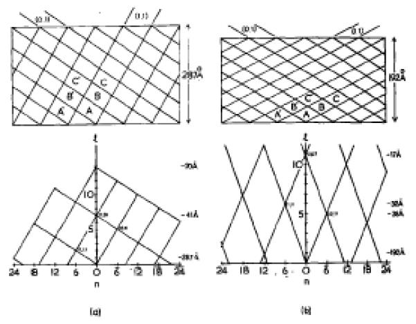
(a) Surface lattice of the extended phage tail. The 6-start families of helices are labelled (0,1) and (1,1) according to the notation of Moody (1973). In the more conventional notation of Klug et al. (1958) for helical surface lattices, these are referred to as (6̅,5) and (6,2), respectively, Successive rings of subunits are labelled with different letters. The lattice is shown with a repeat after exactly seven rings, but moat specimens show small deviations from this: the (0,1) lattice lines (Moody’s “transitional helices”) tend to follow a slightly steeper angle, the (1,1) lines a slightly shallower angle. The annulus spaoing of 41 Å in the extended tail was determined by X-ray diffraction of tail cores (Moody, 1971b), which have been shown by optical diffraction of electron micrographs (Moody, 1971a) to have the same axial spacing as the extended tail sheath. The hand of the lattice has been determined by freeze-etching, by Bayer & Remsen (1970).
(b)(n,l) plot showing the reciprocal lattice of the extended phage tail. For the lattice shown, the selection rule is l = −2n + 7m (where n must be a multiple of 6), although this is only an approximation to the real lattice.
(c) Surface lattice of the contracted phage tail and polysheath which repeats after eleven rings of six subunits. The labelled subunits correspond to those with similar labels in the extended lattice (a), to show the change in relationship between neighbouring subunits during contraction. The “transitional” (0,1) helices of the extended tail have become the “short pitch” (0,1) helices (Moody, 1973). By coincidence, the helical notation is still (6̅,5) for the latter set of helices, although the (1,1) helices have become (6,6) in helical notation. The axial spacing of the annuli in polysheath was also determined by Moody (1967a), who calibrated the optical diffraction patterns from electron microscope images. The hand of the lattice was determined by Bayer & Remsen (1970).
(d) (n,l) plot showing the reciprocal lattice of the contracted tail. The transformation which takes place in the helical surface lattice during contraction is accompanied by a similar lattice transformation (but rotated by 90°) in reciprocal space. The selection rule is l = n + 11m.
Moody (1967a) has also studied the aberrant structure known as polysheath, which is formed by base-plate or core mutants in lysis-inhibited cells, and has proved by optical diffraction the suggestion of Kellenberger & Boy de la Tour (1964), that polysheath polymers have a similar arrangement of protein subunits to the contracted sheath. There is also ample serological and genetic evidence that the contracted tail sheath and polysheath have at least one major protein component in common (To et al., 1969). The latter authors have shown, however, that there are differences in solubility of the two structures in the presence of various dissociating agents, suggesting that the inter-subunit bonding in polysheath is somewhat weaker than in contracted sheath. Moreover, although electron microscope images of tail sheaths which have lost their tail cores appear hollow, polysheath does not (see Plate I). It has been suggested (Moody, 1967a; To et al., 1969), therefore, that polysheath may have some kind of core, of unknown composition, which initiates the polymerization of polysheath.
2. Methods
A mutant phage P19amH21, which is blocked in tail-core formation and therefore forms large amounts of polysheath, was kindly provided by Dr J. King. The lysate, which included phage heads, baseplates and tail fibres as well as polysheath, was fractionated on a 2H2O gradient. Polysheaths, negatively stained with uranyl acatate, were photographed in a Philips EM300 electron microscope at 80kV, nominal magnification 50,000 ×.
Micrographs of negatively stained T4D bacteriophage, in both extended and contracted states, were obtained from Drs J. T. Finch and P. N. T. Unwin.
After selecting the images of suitably well-ordered specimens of each structure by the technique of optical diffraction, each chosen image was digitised using a computer-driven microdensitometer (Arndt et al., 1968) and its Fourier transform computed. The position of the helix axis was refined by intra-particle correlation† of the phases in the two halves of the Fourier transform, corresponding to the near‡ and far sides of the helical structure (see Appendix), and layer lines were extracted by interpolation in the transform array, as described by DeRosier & Moore (1970). The results obtained for a number of structures (see Appendix) suggest that the two sides of the same particle may be differently preserved, although it is not consistently one side or the other which is better. Sets of layer line data (half transforms) from different images were compared (inter-particle correlation) and the best averaged together as described in the Appendix. Individual sets of data were then correlated with the average to determine which had the most in common.
Estimates of the mean radial density distribution, g0(r), of the contracted tails were obtained from end-on views using the computational rotational filtering technique described by Crowther & Amos (1971).
Finally, the three-dimensional density maps were calculated by Fourier–Bessel transformation of the layer line data, as described by DeRosier & Moore (1970), on a grid with points spaced apart by no more than a third of the spacing of the highest resolution data. For example, the maps of the extended tails were calculated on a grid with nominal spacings of 6 Å in one direction and 6·7 Å in the other (the anisotropic spacing being chosen so that an undistorted map could be output on the computer line-printer).
Balsa wood models were built up from sections, at a contour level that was chosen to give continuity in the model. Reconstructed sections were also displayed using a computer-driven cathode-ray tube plotter (Gossling, 1967).
3. Results
(a) Extended tail of T4
Plate I(b) shows a typical optical diffraction pattern obtained from the image of a well-ordered T4 tail. Most such patterns show layer lines out to l = 7 (41 Å), but in the better ones (where the image was not so far underfocussed) layer lines out to l = 14 (20 Å) are detectable. An example of a computed diffraction pattern is shown in Figure 2, which includes many of the higher layer lines. The helical surface lattice, drawn with a longitudinal repeat distance of seven annuli, and the indexing of its diffraction pattern are shown in Figure 1. In most cases, the spacing of the layer lines is not quite regular (see Plate I(b)), indicating that the image does not repeat exactly after seven annuli. Thus, the selection rule l = −2n + 7m (Fig. 1) is only approximate and the diffraction pattern would be better represented by the continuous form of the selection rule (Moody, 1967a): Z = −2n/12p + um/12p, where p is the minor pitch of the basic helix and u the number of annuli in a longitudinal distance of 12p, with n a multiple of 6. The value of u varies between 6·8 and 6·9 from one example to another. If the image repeated after exactly seven annuli, it would contain only 21 different views of the asymmetric unit, and the different harmonic functions in the Fourier transform would be separated from one another to a resolution in the radial direction of about 36 Å. But, in practice, the 18-fold and 24-fold functions that are shown in Figure 1 as lying on the same layer lines (1, 6, 8 and 13) are separated by a small difference in axial spacing. For this reason, it is possible to solve the contributions in each Fourier transform in the radial direction to the same 20 Å limit which is set by the last identifiable layer line in the axial direction.
Fig. 2.

A computer printout of the amplitudes of the computed Fourier transform of an extended T4 tail (particle F), which was densitometered on a raster with a spacing equivalent to about 5 Å. The amplitude peaks have been contoured at a relatively high level at low resolution but at a lower level at high resolution where the background is also much lower. The calculated phases of the main peaks are shown superimposed on them. Lines have been drawn through what appear to be the centres of the layer lines, and the “near side” helical surface lattice has been drawn in roughly to identify the peaks on the layer lines. The 1st, 6th, 8th and 13th layer lines are “split” into two because the longitudinal repeat distance is not exactly 7 annuli as drawn in Fig. 1. The selection rule in this case can be expressed approximately as l = −2n + 6·9m.
Layer line data out to this limit were extracted from each Fourier transform, even if the intra-particle correlation between the phases of pairs of peaks on the two sides of the meridian did not satisfy the normal criterion of being with 45°, which would be applied in the case of reconstructions from individual images. It was hoped that averaging would extract the weak “periodic” signal, corresponding to the rotationally or helically repetitive structure, from the high background noise at high resolution (see Fig. 2). However, it was not possible to identify all the possible layer lines in all of the selected transforms, so one or two whole layer fines were omitted in a few cases.
The data were divided into near and far side contributions (corresponding to left and right halves, respectively, of each layer line for positive values of n; vice versa for negative n), and averaged separately so that separate reconstructions from the two sets of half-transforms could be compared.
Different sets of data correlated well with one another (see Appendix) and showed strong polarity; the residual phase differences when individual half-transforms were compared right-way-up with their average (see Table A1 of Appendix) were between 40° and 65°, with a mean of 52°; the residual differences when the individual half-transforms were compared upside-down with the average were between 80° and 90°, with a mean of 86°. (There was, in any case, no difficulty in orienting all the specimens the same way up because of the presence of attached heads and/or baseplates.) The radial density distributions calculated from the equatorial data of different transforms were also in reasonably good agreement, except near the centre of the structure. They are compared in Figure 3, together with the corresponding mean density profiles from which they were obtained. The equator from one of the more symmetrical particles (B) was selected and used for both near and far side reconstructions. The reasonably good agreement between different specimens for data on other layer lines was confirmed by comparing comparable sections through the individual three-dimensional reconstructions.
Fig. 3.

A comparison of the radial density distributions calculated from different individual extended tails. The left-hand curves are the mean projected densities across each image, averaged along the axis. B and F are the most symmetrical and, of these two, B appears to be the best, since a dip presumably corresponding to the centre of the tail core is resolved at the centre of the density distribution.
The right-hand curves are the mean radial density distributions of the three-dimensional reconstructed images, calculated by Fourier–Bessel transformation of the equatorial data in the Fourier transforms of the original images. The curves all have similar features (i.e. three peala at roughly the same radii) but B appears to be the best; it shows a minimum at the centre corresponding to the hole in the tail core.
Plate II shows contoured sections of the two average reconstructed density maps. The features in the two maps are very similar, although there are differences in detail in the shapes of the contours around the density peaks. The final three-dimensional model is based mainly on the near side map, although interpretation of the structure is based on features in both maps. On the outer surface of the model (nominally about 100 Å radius) there are six helical rows of globular subunits, which follow the (1,1) helices. The subunits within each annulus appear to be in close contact. Further in, at about 70 Å radius, the density is separated by the six helical tunnels described by DeRosier & Klug (1968) which also run parallel to the (1,1) helices. The strongest connections at this radius are along the (1,1) helices. The tail core, with an inner radius of 15 to 20 Å, probably extends out in radius as far as the helical tunnels, although in some sections shown in Plate II it does appear to be somewhat narrower. This interpretation is influenced by Moody’s (1971b) measurement by X-ray diffraction of 90 Å for the core diameter. In fact the variations in density level in the reconstruction are of relatively low amplitude within a radius of about 35 to 40 Å and are probably not significant, since the centre is the least accurate part of the reconstruction.
Plate II.


Sections normal to the helix axis through two average three-dimensional reconstructed images of the extended tail of T4. (Magnification 2,200,000×).
(a) was calculated from averaged “near side” data, (b) from averaged “far side” data. The sections, which are viewed from the head end. are spaced at intervals of 8-2 Å along the axis, so that they repeat after five sections. They are numbered in increasing order from baseplate to capsid. High density represents protein. The contours have been drawn at regular intervals above a lower cut-off level and the peaks are shaded to distinguish them from holes. The resulting plots are thus combinations of the two ways of representing electron density described by Gossling (1967). The contours extend to a nominal radius of about 100 Å. The lowest contour level has been chosen to show clearly the hole in the centre of the tail core and the helical tunnels at 70 Å radius. The proposed boundaries of a single subunit of the sheath are shown as thicker lines superimposed on the contoured sections. They have been chosen to cut through the weaker parts of the map wherever possible. The axial range of the supposed subunit covers more than one 41 Å annulus, since it is slightly tilted. It starts at an outer radius in section 2 and ends at an inner radius in section 8. The annulus of subunits below ends in section 3, while the annulus above starts in section 7. Thus the boundary drawn in each section includes less than one-sixth of the total area. Three views of a three-dimensional model of the proposed subunit are shown in Plate V.
(b) Contracted tail and polysheath
Plate I(d) and (f) show typical diffraction patterns from images of a contracted tail (Plate I(c)) and a stretch of polysheath (Plate I(e)). Layer lines out to l = 6 (32 Å) can be identified in both cases. Their indexing is defined in Figure 1(b). Since the longitudinal repeat distance of 11 annuli includes 33 distinct views, there is theoretically no difficulty in solving the structures to a resolution of 32 Å. However, the contracted tails always appear to be somewhat distorted and are also too short to give a good diffraction pattern. Only layer lines 1, 5 and 6 can be identified in most cases, with the addition of layer line 4 in a few cases. Polysheath occurs in much longer lengths and the consequent improvement in the diffraction pattern allows a few more layer lines to be identified. However, the structure seems to be rather flexible, distorts easily and appears to have a somewhat irregular surface compared with that of the contracted tail sheaths, so that generally the quality of the diffraction patterns is still not as good as for the extended tails.
Contracted tails and stretches of polysheath were correlated with one another and averaged, with the results described in the Appendix. The results for polysheath, where it was necessary to determine the relative polarities of the images from the phase residuals, were fortunately reasonably good. In some cases the relative polarity of two individuals could not be determined by correlating one against the other, but when an average of several individuals, whose relative polarities were unambiguous, was used as reference data all of the previously ambiguous cases were resolved. The residual phases when individual polysheaths were finally compared right-way-up with an average of all the sets of data (Table A2 of the Appendix) were between 25° and 56°, with a mean of 40°†; those when individuals were compared upside-down with the average were between 41° and 72°, with a mean of 58°. The final average set of data, from which the three-dimensional map was calculated, included only the six “best” sets of data selected according to the values of the final phase residuals which averaged 33°.
As in the case of the extended sheaths, the polarity of the contracted tails did not need to be determined from the results of the correlation procedure. This was just as well, since the data in the transform were scarcely adequate for such a determination, the phase residuals tending to be high in both orientations: the residual phases when individual half transforms were compared right-way-up with the final average set of polysheath data were between 36° and 88°, with a mean of 70°; the residuals when they were compared upside-down with the polysheath average were between 61° and 91°, with a mean of 77°. The differences between the results in the two orientations was just sufficient to determine provisionally the polarity of the polysheath data relative to that of the sheath in the actual T4 tail.
The equatorial data were very variable from one image to another, as shown in Figure 4(a) and (b), particularly in the case of the polysheaths. Estimates of the radial density distribution of the sheath in its contracted form were therefore obtained from end-on views of contracted tail sheaths. Images showing the 12-fold spiral appearance described by Moody (1967a) which he interprets as having shrunk at their top ends, were avoided. Of the remaining images, a rotational frequency analysis (Crowther & Amos, 1971) showed which were the most reliable end-on views (Fig. 4(c)), since peaks for the sixfold components (and higher harmonics) were taken to indicate that the particle was well-preserved and was being viewed directly along its axis. Most of the particles analysed in Figure 4(c) satisfy this criterion, but particle A is probably tilted, since the fivefold component is the strongest.
Fig. 4.

Calculations of the mean radial density distribution for contracted tail and polysheath.
(a) Radial density distributions calculated from equatorial data of individual polysheath transforms. Although they are fairly similar near the outside, at inner radii they vary wildly.
(b) Radial density distributions calculated from the equatorial data of individual contracted tails seen side-on, most of whioh still contained a central core. Four of the curves show a peak at 16 to 45 Å, which represents the wall of the core. The sheath is represented by a double peak in most cases.
(c) Mean radial density distributions calculated from contracted sheaths seen end-on on the electron microscope grid, after being separated from their capsid, baseplate and tail core (see Plate I(g) to (j)). The rotational power spectra (Crowther & Amos, 1971) on the far right are a guide to whether or not the view is exactly down the axis. A direct view of an undistorted specimen should give peaks at n = 0, n = 6 and n = 12, but not in between. Since the images did not have very strong azimuthal modulations, the peak at n = 0 is much larger than the other peaks. The last example was considered to be reasonably good and was used in the three-dimensional image reconstructions of the contracted tail and polysheath, after being scaled to a similar level to the radial density distributions caloulated from side-on views ((a) and (b)).
The noisy quality of the data from side-on views is borne out by comparisons of equivalent sections through the individual three-dimensional reconstructions (not shown). The polysheath maps are in best agreement at outer radii, but tend to vary a great deal farther in. However, there are consistent features in several examples. None of the contracted tails produced a three-dimensional map with very much detail, apart from a set of knobs on the outer surface. It was therefore considered not worthwhile to calculate an average reconstruction.
Plate III shows contoured sections through the reconstructed density map obtained from an average of the six best sets (half-transforms) of polysheath data, combined with the radial density distribution shown for particle D in Fig. 4(c). The “polycore” in the centre of the sheath, if it really exists, has thus been eliminated from the reconstructed density. Plate IV(b) shows a model constructed from these sections. The contour level chosen for the model gives an outer diameter of about 250 Å. The inner radius of the sheath in the model is about 70 Å and the model shows relatively little variation in density at this radius. Further out it is cleaved strongly into 12 helical columns in the direction of the (2,1) helices. On the outside, a row of globular subunits is attached to one side of each column.
Plate III.

Sections normal to the helix axis through the average three-dimensional reconstructed image of T4 polysheath, including the radial density distribution from an end-on view of a contracted tail, which has produced the hole in the centre of the model. (Magnification 1,500,000×.) The sections are spaced at intervals of 8·7 Å along the axis, so that alternate sections are similar. They are viewed from what is thought to be equivalent to the capsid end of the structure and are numbered in increasing order from baseplate to capsid ends. The densities are represented by a combined contour and density plot, as in Plate II. The boundaries of the subunits are fairly obvious at the outermost radii, but are more difficult to distinguish at inner radii. The possible boundaries of three neighbouring subunits in different rings have been drawn in and labelled A (dotted boundary), B (thick solid lines) and C (dashed boundary). Continuity of the subunits from section to section has been used as a criterion in choosing the boundaries. Neighbouring annuli of subunits appear to interdigitate much more than in the extended structure, so that each section includes sections through at least 12 subunits. An isolated subunit constructed from these sections is shown in Plate V.
Plate IV.

Views of models representing the three-dimensional reconstructed images of T4 extended tail and polysheath. Each model consists of 12 annuli and thus corresponds to half of a complete phage tail. The outer knobs of some of the subunits are labelled to show the lattice transformation (of Fig. 1). The upper surfaces of the models have been finished off in accordance with the interpretation of the subunit boundaries shown in Plates II and III, to represent the top surfaces of individual annuli of subunits. The subunits are shown in more detail in Plate V. In the model of the extended tail (a) a short continuation of the tail core is shown. Magnification 2,400,000×.
4. Discussion
The quantitative information, which is obtained by correlating the data as described in the Appendix, appears to be very useful in selecting the best images, and even the best “sides” of different images. Since one side is in contact with the carbon support and the other is not, the two sides are differently stained and undergo different distortions (Moody, 1967a, 1971). It is not unusual, therefore, for one side of the structure to be significantly better preserved than the other, although the results obtained for the final selected particles of several different structures (see Appendix) suggest that, on average, the two sides are equally good. It is not obvious that this should be so. Klug & Berger (1964), in their original work on optical diffraction of electron micrographs, discovered that particles in negative stain are usually coated on both sides, but found that often the spacings on one side appeared to be greater than those on the other. Moody (1967a) confirmed this for T4 polysheath and deduced that in shallow stain the side furthest from the carbon substrate (the far side, by our convention) tended to shrink (by as much as 40%) more than the side in contact with the carbon. One might expect, therefore, that the near side would be consistently better preserved than the far side. However, although the relative spacing of the two sides was not used as a criterion in selecting the images used in the present work, the images finally chosen tended to have fairly similar spacings on their two sides (see Table A2, for example). Transforms that appeared grossly asymmetrical mostly showed poor phase correlation with other transforms. We deduce that both sides are better preserved from distortion in deeper stain. Nevertheless, there may be slight differences between near and far side reconstructed images, as discussed later.
(a) Extended tail
Comparison of the new model of the extended tail with the earlier reconstruction of DeRosier & Klug (1968) shows differences at the outer surface of the sheath; the large protruding subunits no longer have an extension of weaker density trailing away from them in a clockwise direction around the sheath. The extra density at the outside of the old model may represent a real feature, possibly an occasional tail fibre lying in the groove or a fine extension of the tip of each subunit, whose position varies according to the staining conditions and thus averages out when different images are combined. However, for present purposes, this weak feature can be ignored and the new model is designed to show the regions of strongest density. It is worth noting that its outer surface agrees quite well with the low-resolution model of the extended tail of T6 reconstructed by Mikhailov & Vainshtein (1971).
The final reconstructed density (Plate IV(a)) is based mainly on the near side reconstruction (Plate II(a)), which shows features at inner radii most clearly, but details at outer radii of the far side reconstruction (Plate II(b)) are also taken into account. Since the near side is the one closest to the carbon support film, it is possible that the tips of the subunits on this side of the particle tend to be flattened, giving rise to the observed differences between the near and far side reconstructions at the outermost radii.
In order to be able to compare this structure with that of the contracted sheath, it is desirable to distinguish the individual subunits of the extended sheath. An attempt to divide the structure by following the course of regions of highest density is illustrated in Plate II. The heavy lines show the boundary, in each section, of what is thought to be an individual subunit. There are obvious difficulties in trying to interpret the internal structure of a negatively stained aggregate, since there is no reason to suppose that the stain will provide contrast in regions where adjacent subunits are in contact. Fortunately, in the case of the extended tail, the substantial helical tunnels allow stain to penetrate between the subunits at inner radii. Thus the boundaries between subunits are fairly clear except in two regions: (i) in the axial direction the density is continuous at inner radii along the (1,1) helices; (ii) the globular projections on the outer surface appear to be connected azimuthally to regions of high density on both sides. In Plate II the subunit boundaries shown are those judged to be the most likely to represent the true subunit. At inner radii the subunits have been separated between sections 1 and 2; at outer radii, the globular projections have been assigned towards the left, producing subunits that spiral in an anticlockwise directions when viewed from above. Each subunit slopes slightly downwards on going from inner to outer radii. Views of individual subunits, according to this interpretation, are shown in Plate V.
Plate V.

(a) Models of individual subunits of extended and contracted sheath as interpreted in Plates II and III. Three views of the extended subunit and one of the contracted subunit (far right) are shown. Magnification 3,600,000×.
(b) and (c) Close-up views of the models of the extended and contracted structures showing the three-dimensional relationships between the subunits in more detail. Magnification 3,000,000×.
(b) Contracted sheath, and polysheath
As described above, the polysheath and contracted tail data are not as good as those obtained for the extended tail, even though long lengths of polysheath were available. Data for contracted tails were particularly poor. We have therefore assumed the structure of polysheath to be representative of the contracted sheath at the present resolution. Although a difference has been found in the strength of inter-subunit bonding between contracted sheath and polysheath, in view of the similarity in appearance and the fact that data from the two structures correlate together reasonably well (see Table A2 of the Appendix), the differences in structure are unlikely to be grossly different. One might expect the greatest difference to occur near the centre of the sheath, since in the case of polysheath the normal sheath-core interaction will not have taken place.
The outer contour of an end-on view of the reconstruction agrees well with end-on views of contracted tails and pieces of polysheath (Moody’s “pineapple sections”, 1967a). The appearance of the outer surface of the reconstruction is also in agreement with pictures of freeze-etched contracted tails shown by Bayer & Remsen (1970). It is likely, therefore, that the outer surface of the model is reasonably accurate. The boundary of the outer half of an individual subunit is not difficult to decide (Plate III). When this boundary is compared with the subunit boundary chosen for the extended structure (Plate II), the two shapes are seen to be remarkably similar (see also Plate V). Both structures show the same fist-like projections at their outer tips. Moreover, in both structures, the “arm” which ends in the fist exhibits an “elbow”, which causes the arm to slew in the same direction. This similarity suggests that the relative polarity, as determined by comparison of polysheath and contracted tail data, is probably correct.
The accuracy of features at radii of less than about 60 Å is difficult to assess. Although there is close agreement at outer radii between individual reconstructions, at inner radii there are significant variations in the density distribution between one individual and another. In many cases the block of density between the arms is broken up into two or three separate peaks, but since the positions of the peaks vary from one individual to another, the details are smoothed out in the average. Taking this into account, the boundaries shown in Plates III and V define the most likely shape for the whole subunit at the present resolution. It is unfortunate that the inner half of the contracted subunit is so poorly represented.
The volumes of the subunits in the two models are unequal, but the difference can be accounted for by the greater radial shrinkage in negative stain of the contracted structure. To agree with the results from freeze-etching (Bayer & Remsen, 1970), radial distances in the model of the extended structure must be increased by a factor of 1·18, whilst the polysheath model requires a factor of 1·38. After scaling in this way, the volume of a sheath subunit in the model of the extended tail is approximately 95,000 Å3 (or 76,000 daltons, assuming a density of 0·8 dalton/Å3), and in the polysheath model the calculated volume after correcting for shrinkage is about 106,000 Å3 (85,000 daltons). The volume of the core in the extended tail is also similar to what one would expect, assuming a one-to-one ratio of core to sheath subunits: with corrected inner and outer radii of 20 Å and 45 Å, respectively, the volume per subunit would be 34,000 Å3 (27,000 daltons for a density of 0·8 dalton/Å3). At present, however, the dimensions of the core can only be regarded as approximate.
(c) Comparison with baseplates
End-on views of unattached extended baseplates have been rotationally filtered to reveal their structure in fine detail (Crowther & Amos, 1971). The extended baseplate is believed to act as a template for tail assembly (see e.g. King & Mykolajewycz, 1973). It is possible that the manner in which the first annulus bonds to the baseplate is similar to the way each successive annulus bonds to the one below. This idea is supported by the images shown in Plate VI, which shows that there is a strong degree of similarity between the end-on views of the uncontracted baseplate and an annulus of the extended tail. Plate VI(a) is a section through the reconstructed three-dimensional image of the extended tail which is fairly representative of the projected view of a whole ring of molecules, while Plate VI(c) is a contoured filtered image of a baseplate. Plate VI(b) shows the tail section superimposed on the central part of the baseplate. There is, however, as yet no evidence that this relative angular positioning of the tail and baseplate is the one that actually occurs.
Plate VI.

Comparisons of sections of the extended phage tail and polysheath with baseplates in extended and contracted forms. Magnification 1,300,000×.
(a) A section through the centre of an annulus of subunits in the near side three-dimensional reconstructed image (see Plate II(a)), viewed from above. This is fairly representative of the density distribution normal to the axis throughout the whole annulus.
(b) Contours of the tail section shown in (a) superimposed on the filtered baseplate image shown in (c). The inner parts of the sheath subunits fit closely on to the central structure of the baseplate.
(c) Rotationally filtered image of an extended baseplate (Crowther & Amos, 1971). The top surface of the baseplate is believed to have been in contact with the carbon substrate of the electron microscope grid, and therefore faces upwards in this print (R. A. Crowther, personal communication).
(d) A section through the centre of an annulus of subunits in the polysheath three-dimensional reconstructed image (see Plate III), viewed from above.
(e) Rotationally filtered image of a baseplate in the contracted form (J. King & R. A. Crowther, unpublished work). None of the polysheath sections in Plate III can be made to superimpose well on the baseplate image.
(f) Contours of the extended baseplate superimposed on the contracted baseplate image. The central parts of the two structures are very similar although there are marked changes in density distribution at the periphery. The lack of transformation of the central structure during contraction explains the difficulty in fitting the sections of contracted sheath on to the baseplate image.
It has not been found possible to fit the filtered image of an isolated contracted baseplate (Plate VI(e), J. King & R. A. Crowther, unpublished work) to any section of the contracted structure (e.g. Plate VI(d)) in the same way. In fact, the central part of the contracted baseplate still strongly resembles the centre of the extended baseplate, although considerable changes have occurred at the periphery (Plate VI(f)). In other words, although the central part of the unattached baseplate mimics a ring of the tail sheath (and core) in the extended form, the contracted form does not appear to have undergone the same change in configuration as the sheath undergoes during contraction. There are two most probable explanations for this difference. Either (i) the change in the sheath during contraction is induced mainly by movement of the outer parts of the baseplate, or by movements in the z-direction of the central part of the baseplate, which would not show up in projection and which cause the centre of the first annulus to lose contact with the baseplate; or (ii) the transformation is not complete in free baseplates which are artificially induced to contract. There is no way at present to decide between these two alternative explanations.
(d) The contraction process
Moody’s (1973) analysis of the process of contraction has shown how the lattice of the contracted tail (and polysheath) is derived from that of the extended tail. Thus we can relate the relative positions of neighbouring subunits in the two structures, as shown in Figure 1 and Plate IV. Azimuthal contacts are probably broken at all radii before the sheath can contract, since the distance between A and A′ increases considerably. On the other hand, as Moody has established, the distances AB and AB′ do not change very much, so it is quite likely that contacts in these two directions are maintained, at least at some radii. If so, connections between subunits in the sheath along these directions would, as a first approximation be analogous to those between the levers of a pair of lazy-tongs.
Comparison of the two reconstructed images (Plates IV and V) and of the subunit boundaries deduced from them (Plates II and III) suggest that the large change in the gross structure during contraction may be effected by a relatively small change in the overall shape of the individual subunits. But the orientation of the subunits relative to the helix axis changes. There appears to be a movement of the whole “arm” which causes the “fist” to swing outwards, breaking its contact with the next subunit in the same ring. There is also a slight change in angle relative to the axis, since the arm points slightly downwards in the extended structure, but appears to be more nearly horizontal in the polysheath. There must of course be an internal conformational change which accompanies the change in angle between the two “preserved” bonds with neighbouring subunits (AB and AB′). The distribution of density in the two models suggests that the AB bond at an intermediate radius (about 60 Å in the extended sheath, which becomes 90 Å in polysheath) and the AB′ bond at the innermost radius of the sheath might be preserved during contraction. The preservation of both these contacts could most easily be achieved by twisting the two parts of the subunit relative to one another at some radius between these two points.
Moody’s (1973) results showed a change in the appearance of tail sheaths that had just started to contract, but had been fixed before they could shorten significantly. The lateral striations became much less pronounced, while the oblique striations corresponding to the “transitional” helices (see Fig. 1) became more obvious. (A similar effect has been observed by Donelli et al. (1972) in images of the tail of bacteriophage G.) This suggests that at least part of the conformational change is effected before the actual contraction. The breaking of the azimuthal bonds described above is likely to be included in this pre-contraction change, since one would expect this to give rise to precisely the change in appearance that is observed, because of the further penetration of stain between subunits in the same annulus, accentuating the helical grooves.
The process of contraction, as envisaged by Kellenberger & Boy de la Tour (1964), Moody (1967b, 1973), To et al. (1969) and others, can be discussed in terms of the structures described, as follows. A change in the structure of the base plate which initiates the contraction produces the required conformational change in the bottom annulus, which weakens the intra-ring bonds, as well as bonds between sheath and core. The change in conformation is transmitted up the sheath from annulus to annulus, leaving the transformed part of the sheath in a “tense” state which To et al. (1969) have likened to a “suspended spring”. At some point, the tension due to the changes in conformation of a sufficient number of annuli would push the core through the baseplate, and a wave of contraction, triggered by the expansion of the baseplate, would follow the wave of conformational change. During contraction each ring would be forced to expand radially by the expansion of the ring below. At the same time, each subunit, being still bonded to both neighbours in the ring below, would be pulled down into the gaps which appeared between subunits in the lower ring, thus producing the fully contracted conformation.
Acknowledgments
We are grateful to Drs R. A. Crowther and J. T. Finch for advice and discussions during the course of this work. We also thank Drs J. T. Finch and P. N. T. Unwin for electron micrographs of T4 tails, Drs R. A. Crowther and J. King for unpublished filtered images of baseplates, and Drs J. E. Mellema, P. N. T. Unwin and T. Wakabayashi for allowing us to quote results of theirs in the Appendix.
APPENDIX. Combination of Data from Helical Particles: Correlation and Selection
Electron micrographs of negatively stained biological structures have a high level of background noise from irregularities in the stain and in the support film. The way to filter out most of this random background is to average the signal from many independent copies of the same structure. The process of three-dimensional image reconstruction of a subject with helical symmetry (DeRosier & Klug, 1968) produces an average image of all the subunits in the length of the structure under investigation; but normally the amount of averaging is limited either by the fixed lengths of the particles themselves or by the relatively short stretches over which long particles remain straight on the electron microscope grid. Further averaging has to be achieved by combining the data from several different specimens, for which the relative orientations must first be found. Fortunately, in the case of most helical structures, the image (and its Fourier transform) varies in a predictable way with changes in view angle and it is possible to correlate data from different images selected at random, and thereby determine their relative view parameters.
The procedure for correlating the two halves of a helical transform in regions where there is no overlap of different Bessel functions has been discussed in detail by DeRosier & Moore (1970). This process, which one might refer to as intra-particle correlation, depends on the fact that the transform of each image provides two more-or-less independent measurements of values in the three-dimensional transform (i.e. the values on each layer line on opposite sides of the meridian). Except where n = 0, the two values are associated with either the near side or the far side of the helical structure. As far as possible, we process the two sets of values corresponding to the near and far sides separately, since one side may be better preserved than the other.
(a) Residual maps
Assuming the directions of the helix axis, in each of two images, have already been found by self-correlation of the transforms, the relative orientations can be described in terms of Δz, the relative shift along the axis, and Δϕ, the difference in azimuthal angle. The expected difference in phase at corresponding points along a particular layer line, of meridional spacing Z, in the two transforms is
where n is the order of the Bessel function on that layer line (see Klug et al., 1958).
In order to determine the values of Δϕ and Δz we may compare the actual differences at a number of different points in the transform with those expected for particular values of Δϕ and Δz, and compute residual maps such as those shown in Figure A1. A minimum in the map should correspond to the most probable values of Δϕ and Δz. The value of the minimum provides an indication of the degree to which the two transforms agree, provided all relevant parts of the transform are included in the correlation. In practice it is not always possible to identify a particular layer line in every transform. If possible, a transform which includes a complete set of recognizable layer lines is chosen as the reference, and in computing the residual maps for other transforms a penalty is imposed for any missing data (see below).
Several different residual functions have been experimented with. One is the least-squares residual
where F2′ = F2 exp [i(−nΔϕ + 2π + ZΔz)], and F1 and F2 are corresponding complex values in the two Fourier transforms.
Fig. A1.

Regions of typical residual maps close to the minimum values. In this case the residual maps were calculated by comparing the near-side data from an extended phage tail (particle F in Table A1) with the average from six nets of data, (a) The phase residual R(Δϕ,Δz), weighted as described in the text; (b) the least-squares residual S(Δϕ,Δz).
The results from such a residual map have proved satisfactory in providing a single distinct minimum corresponding to what appear to be the correct values of Δϕ and Δz. However, its absolute value is very sensitive to differences in the scale of the amplitudes of the two data sets being compared. In practice, the intensities in diffraction patterns from negatively stained particles are fairly variable from one image to another, since the stain thickness and degree of stain penetration into the structure are different from particle to particle. The diffraction peaks on opposite sides of the meridian may differ significantly in amplitude. Yet the correlation between the phases may be very good in such cases. Thus, a weighted “phase residual” tends to provide a more objective measure of the degree of correlation between two particles.
For internal correlation of a particular transform, DeRosier & Moore (1970) defined the parameter Q:
where Δθ is the difference between the observed and expected relative phases. Weighting with the mean amplitude ∣F∣ allows the stronger and more reliable peaks to dominate the result.
The problem is slightly different when one is comparing different images. In the case of many helical structures, such as the T4 polysheaths, it is not possible by eye to distinguish one end of the particle from the other, so the relative polarity of two different specimens, as well as Δϕ and Δz, must be determined. Since the lower resolution reflections, which are generally the strongest in the transform, tend to contain little information about the polarity of the structure, it is better to reduce their influence by using an expression with lower amplitude-weighting:
where Δθ = θ2 – θ1 – nΔϕ + 2πZΔz – k2π and k is an integer such that −π ≤ Δθ ≤ π. If a layer line cannot be identified in a particular transform, Δθ is set to 90° for all the missing data points.
The most probable relative polarity of the two structures is determined by comparing the residual map with a second one (R* (Δϕ, Δz)) calculated with one of the particles turned upside-down. This operation is equivalent to changing ϕ to −ϕ and z to −z, which can be simulated in practice by substituting −θ2 for θ2 in the above expression and searching for a new minimum as a function of Δϕ and Δz.
A further parameter that may vary is the relative radial scaling of the two transforms. Different particles seem to stretch or shrink by different amounts in the negative stain. The magnification may also vary slightly from plate to plate. In searching for the best radial scaling factor, it is important to try to match the amplitudes as well as the phases, since the latter may be approximately constant over long stretches of the layer line. In this respect, the least-squares residual is very useful. Thus, the two residuals S and R are complementary and the fitting procedure is performed taking both into account. Fortunately there is not usually any conflict between the two.
(b) Averaging of data
Once the relative polarities and values of Δϕ, Δz and the radial scaling factor have been found for a number of images, using a particular image as the reference data, it is an easy matter to average the layer line data. The phases are corrected for the differences in orientation, and the differences in radial scale compensated for by linear interpolation to provide values at equivalent points in each transform. To allow for differences in the scale of intensities, the data were weighted so that the average intensity along a particular layer line would be the same in all transforms. In practice the weights required varied between 0·5 and 1·5.
(c) Results for T4 extended tail
The results obtained by fitting different phage tail images together are fairly typical. Each residual map showed a single sharp minimum, so that with data out to 20 Å resolution the fit was made to within 1° in ϕ and 1 Å in z. Figure A1 shows part of a typical residual map in the region of the minimum.
Table A1 summarizes the results for all the particles included in the final selection. The first column shows the results obtained when one of the individual transforms was chosen as the reference set of data. The first value given (Rmin) is the minimum phase residual obtained when the two particles are in the same orientation. The second value () is the minimum residual with the second particle turned upside-down. Near and far sides were correlated separately but the results are very similar in both cases. The radial scaling factors for these highly selected particles proved to be very similar for the two sides of each particle. It is clear that the “upside-down residual”, is greater in all cases than Rmin, the “right-way-up residual”, by up to 35°, although in one case the difference is only 3°. This proves that with data of this quality it is possible to determine relative polarities unambiguously. When the different sets of data are averaged and the average used as reference, the differences between Rmin and become even more marked, the smallest difference now being 24°, the largest 58°. This mainly reflects reductions in the values of Rmin. Obviously the average set of data has considerably less random noise than the original reference, and the residual phase differences must now be due predominantly to errors in the individual data sets with which it is being compared. Similar reductions in Rmin are obtained whichever of the individual particles is used as the original reference data. A reduction in Rmin is observed even for particles which were not included in the average used as reference in the second round of correlation (see Table A2(a), for polysheaths).
Table A1.
Phase-residuals† from, inter-particle correlation of T4 extended tails
| Particle A as ref. Rmin/ (°) |
Average 1 as ref. Rmin/ (°) |
Average 2 as ref. Rmin/ (°) |
Twofold residual () (°) |
|
|---|---|---|---|---|
| (a) Near sides | ||||
| A. (796–23F) | — | 40/80 | 42/80 | 86 |
| B. (642–7A) | 54/82 | 43/85 | 43/85 | 82 |
| C. (23770A) | 72/90 | 61/88 | 61/88 | 91 |
| D. (796–23C) | 70 78 | 53/87 | 50/87 | 91 |
| E. (796–23A) | 65/82 | 51/82 | 60/82 | 93 |
| F. (641–3A) | 57/88 | 43/90 | 42/90 | 83 |
| Average 2 (near) | — | — | — | 86 |
| Average 2 (far) | — | — | 55/85 | — |
| (b) Far sides | ||||
| A. (796–23F) | — | 41/89 | 43/87 | 89 |
| B. (642–7A) | 53/88 | 45/80 | 46/80 | 90 |
| C. (23770A) | 82/85 | 65/89 | 65/89 | 81 |
| D. (796–23C) | 63/87 | 50/89 | 50/89 | 83 |
| E. (796—23A) | 59/88 | 43/87 | 43/87 | 87 |
| F. (641–3A) | 72/90 | 57/88 | 58/88 | 88 |
| Average 2 | — | — | — | 88 |
Including data to 20 Å resolution. With a resolution cut-off of about 32 Å, which would exclude the weaker parts of the transform (as in the case of the contracted structures, see Table A2), the values of Rmin would be much lower.
Table A2.
Phase residuals† from inter-particle correlation of T4 polysheaths and contracted tails
| Particle A as ref. Rmin/ (°) |
Polysheath average as ref. Rmin/ (°) |
Radial scaling factor | Twofold residual () (°) |
|
|---|---|---|---|---|
| (a) Polysheaths | ||||
| A. (17908A)near | 39/70 | 37/72‡ | 1·04 | 71 |
| (17908A)far | — | 25/63‡ | 1·00 | 87 |
| B. (17913D)near | 47/67 | 54/64 | 1·04 | 57 |
| (17913D)far | 45/67 | 43/65 | 0·94 | 94 |
| C. (17909A)near | 55/48 ? | 46/60 | 1·07 | 51 |
| (17909A)far | 43/54 | 37/51‡ | 1·08 | 72 |
| D. (17914B)near | 42/41 ? | 26/41‡ | 1·06 | 51 |
| (17914B)far | 48/52 | 39/49‡ | 1·06 | 49 |
| E. (17913A)near | 65/65 ? | 56/59 | 0·97 | 58 |
| (17913A)far | 43/68 | 34/60‡ | 0·99 | 71 |
| Average data | —/— | —/— | 60 | |
| (b) Contraoted tails | ||||
| A. (9210A)near | 38/75 ? | 74/84 | 1·08 | 61 |
| (9210A)far | — | 75/76 | 1·08 | 78 |
| B. (9230A)near | 70/68 ? | 36/55 | 1·12 | 72 |
| (9230A)far | 54/61 | 47/61 | 1·12 | 56 |
| C. (9193A)near | 66/50 ? | 77/88 | 1·06 | 72 |
| (9193A)far | 38/58 | 75/73 ? | 1·10 | 56 |
| D. (9210B)near | 46/60 | 84/88 | 1·03 | 69 |
| (9210B)far | 63/47 ? | 64/78 | 1·06 | 78 |
| E. (9199A)near | 35/61 | 81/82 | 1·09 | 66 |
| (9199A)far | 61/67 | 88/91 | 1·02 | 65 |
A question mark indicates Borne doubt about the polarity at this stage in the analysis. Polysheaths C Bnd D were therefore not included in the average that was used as reference for the second round of oorrelation.
Including data to a resolution of 32 Å.
Included in the final polysheath average.
The average obtained in this way is naturally somewhat biased towards the original reference particle. This bias is difficult to avoid using the simple techniques described here. But more sophisticated methods of correlation do not seem to he worthwhile in terms of the computer time they would require for the small gains. However, the bias can be reduced slightly by regarding the first average as merely provisional and calculating a second average. The values of Δϕ and Δz at which Rmin occurs may differ slightly between the first and second rounds of phase correlation, so a new average may be calculated based on the new relative orientations (see column 3 of Table A1). Further rounds of correlation and averaging have, in general, not been found to be worthwhile, except in cases where data from more particles can be included at each stage (as for polysheaths below; see also Wakabayashi et al., 1975).
(d) Results for polysheaths
In this case it was necessary to determine the relative polarity of different specimens from the residuals Rmin and . The first column of residuals in Table A2(a) shows the results of fitting each side against a particular set of data chosen as the reference: the two sets of residuals are classified as Rmin or according to the final results of the polarity determination (column 2). From the first set of results (column 1) it was not possible to be sure of the relative polarities of three of the particles, since the two sides of each transform gave different results. However, these ambiguities were resolved using an iterative procedure of correlating against successive averages of all the particles with unambiguous relative polarities. Each cycle improved the values of Rmin slightly and allowed more images to be included in the average, until eventually the relative polarities of all the particles were known (2nd column of residuals in Table A2(a)). Radial scaling factors tended to be slightly different for the two sides of the same particle.
(e) Results for contracted tails
The results for T4 contracted tails are much worse than for either of the previous structures, perhaps because the reflections are derived from such short lengths of tail. Fortunately, the polarity of each image was known beforehand from the presence of an attached head and/or baseplate. In the first column of Table A2(b) are residual values obtained with one side of an individual contracted tail as reference. Values of Rmin are no lower on average than those of . The second column shows the results obtained by correlation with the final set of polysheath data. The differences between Rmin and , although small, are consistent in sign and thus determine the polarity of the polysheath reconstruction relative to the normal tail sheath. However, it did not seem worthwhile to continue the analysis of the contracted tails themselves as far as an average three-dimensional reconstruction.
(f) Comparison of phage tail results with those for other structures
A convenient way of summarizing the results of the fitting procedure is to plot values of Rmin against the corresponding values of . Figure A2 shows several examples of such plots for different structures studied in this laboratory. In each case they are the minimum residual values obtained by comparing the individual data sets with their average. For a non-polar structure, one would expect values of Rmin and to be similar, so plotted points should lie close to the diagonal line in this case. This is clearly true for the haemocyanin aggregate (Fig. A2(h)), whose two halves are believed to be related by a dyad (Mellema & Klug, 1972). The other examples are of structures which are believed to be polar. The distances of the plotted points above the diagonal line provide an indication of the degree of polarity inherent in the data.
Fig. A2.

Polarity plots for different sets of layer line data. The results (Rmin) of correlating the phases of each set of data with those of a reference data set are plotted against the equivalent result () obtained with the reference turned upside down. The results for a non-polar structure should lie close to the diagonal line (e.g. (h) haemocyanin). For polar structures ((a) to (g)) the distance of the points above the diagonal line provides an indication of the degree of polarity present in the data, (a) Extended phage tail (1), was calculated by correlating each set of data with a chosen individual set. (b) Extended phage tail (2), was the result of correlating each data set with the average data. Notice the significant reductions in Rmin, indicating a reduction in random error in the average, while the values of remain much the same as before. The results shown for the other structures ((c) to (g)) were obtained by correlating against their average data sets. The small arrows on the ordinate of each plot indicate the average values of the 2-fold residual (see text) which are closely similar to the corresponding values of . For (a) and (b), see Table A1; for (c) and (d), see Table A2; for (e) and (f), see Wakabayashi et al. (1975); and for (g) and (h), see Table A3.
TMV, tobacco mosaic virus; Tm, tropomyosin; TnT, troponin T; TnI, troponin I.
The values of the minimum phase residuals (Rmin) provide a rough indication of the relative reliabilities of different reconstructed density maps. Thus, of the maps for which data are shown in Figure A2, the reconstruction of the stacked disk of TMV protein (Unwin & Klug, 1974) is the most reliable, while the T4 extended tail, T4 polysheath and muscle thin filaments are all of similar quality; note, however, that the maximum resolution of the data included is not the same in all of these maps. As mentioned above, the intensity on a particular layer line in different transforms is rather variable, so in absolute terms the errors in amplitude in the reconstructed density maps are quite large. But these errors will not necessarily affect the positions of the major features and will not have too much influence on the interpretation of the maps. However, investigations are at present being made into more quantitative ways of assessing the level of error in three-dimensional density maps reconstructed from electron microscope images.
Table A3.
Phase residuals from inter-particle correlation of haemocyanin and stacked disks of tobacco mosaic virus (TMV) protein
| Average data as ref. Rmin/ |
Two-fold residual () (°) |
|
|---|---|---|
| (a) Haemocyanin, to about 58 Å resolution (Mellema & Klug, 1972) | ||
| A. (16269)near | 47/51 | 51 |
| (16269)far | 48/51 | 56 |
| B.(16315)near | 42/44 | 53 |
| (16315)far | 42/46 | 53 |
| C. (16312)near | 52/53 | 67 |
| (16312)far | 48/46 | 64 |
| D.(16618)near | 62/99 | 61 |
| (16618)far | 62/99 | 61 |
| Average | —/— | 40 |
| (b) Stacked disk of (TMV) protein, to about 10 Å resolution (Unwin & Klug, 1974)† | ||||
| J0 | J17 | J0 | J17 | |
| A. | 30/45 | 35/73 | 53 | 81 |
| B. | 41/47 | 37/63 | 52 | 66 |
| C. | 40/52 | 36/72 | 64 | 84 |
| D. | 25/48 | — | 68 | — |
| E. | 41/52 | 32/65 | 61 | 86 |
| Average | —/— | —/— | 45 | 72 |
Layer lines of zero order (J0) and 17-fold (J17) contributions from each transform were correlated independently in this case, to give separate phase residuals. This was done to determine the relative polarities more accurately, since the azimuthal data (J17 contributions) are more strongly polar than the axial variations (J0).
(g) Twofold residuals
A particular application of the phase fitting process is in the comparison of a particle with itself turned upside-down, in order to search for 2-fold axes normal to the helix axis. In practice this is most easily done by finding the orientation in which the layer line data would be closest to being entirely real, that is, where the phases are closest to either 0° or 180°. A similar sort of phase residual to the values of obtained by comparing different particles in opposite orientations, can be calculated, and the value of the minimum should give some indication of whether or not the structure has 2-fold symmetry. (In fact, the values of the minima in the 2-fold residuals compare well with values of (see Tables A1, A2 and A3).) However, it would be difficult to judge from the 2-fold residuals alone whether the structure has 2-fold symmetry or not; a high residual could be due either to random error, to genuine polar information or to a combination of both. The two effects can be distinguished to some extent by comparing the 2-fold residuals of the individuals with that of their average. If the latter is significantly lower, as in the case of haemocyanin (Table A3(a)), it provides an indication of 2-fold symmetry. Notice that the average of the extended phage tails (Table A1) appears to be no less polar than any of the individuals. However, in general, comparison of the phase-residuals Rmin and , as in Figure A2, provides a more satisfactory answer to the question.
Footnotes
The terms “intra-particle correlation” and “inter-particle correlation” will be used to distinguish between correlation of the phases within an individual transform (on opposite sides of the same layer line, in the case of a structure with helioal symmetry) and correlation of the phases between half-transforms from different images (see Appendix).
With the conventions we have used, the “near” side is the side of the particle in contact with the support grid. All micrographs etc. are printed so that the specimens are viewed with the “near” side uppermost.
These relatively low residual phases appear to be better than those for the extended tails, but this is because the resolution cut-off in this case is 32 Å rather than 20 Å. Notice that the “upside-down” residuals are also lower.
REFERENCES
- Amos LA, Klug A. J. Cell Sci. 1974;14:523–549. doi: 10.1242/jcs.14.3.523. [DOI] [PubMed] [Google Scholar]
- Arndt UW, Crowther RA, Mallett JFW. J. Scient. Instrum. 1968;1:510–516. doi: 10.1088/0022-3735/1/5/303. [DOI] [PubMed] [Google Scholar]
- Bayer ME, Remsen CC. Virology. 1970;40:703–718. doi: 10.1016/0042-6822(70)90215-1. [DOI] [PubMed] [Google Scholar]
- Crowther RA. Phil. Trans. Roy. Soc. London. 1971;261:221–230. doi: 10.1098/rstb.1971.0054. [DOI] [PubMed] [Google Scholar]
- Crowther RA, Amos LA. J. Mol. Biol. 1971;60:123–130. doi: 10.1016/0022-2836(71)90452-9. [DOI] [PubMed] [Google Scholar]
- Crowther RA, Amos LA, Finch JT, DeRosier DJ, Klug A. Nature (London) 1970;226:421–425. doi: 10.1038/226421a0. [DOI] [PubMed] [Google Scholar]
- DeRosier DJ, Klug A. Nature (London) 1968;217:130–134. [Google Scholar]
- DeRosier DJ, Moore PB. J. Mol. Biol. 1970;52:355–369. doi: 10.1016/0022-2836(70)90036-7. [DOI] [PubMed] [Google Scholar]
- Dickson RC. Virology. 1974;59:123–138. doi: 10.1016/0042-6822(74)90210-4. [DOI] [PubMed] [Google Scholar]
- Donelli G, Guglielmi F, Paoletti L. J. Mol. Biol. 1972;71:113–125. doi: 10.1016/0022-2836(72)90341-5. [DOI] [PubMed] [Google Scholar]
- Gossling TH. Acta Crystallogr. sect. A. 1967;22:465–468. [Google Scholar]
- Kellenberger E, Boy de la Tour E. J. Ultrastruct. Res. 1964;11:545–563. doi: 10.1016/s0022-5320(64)80081-2. [DOI] [PubMed] [Google Scholar]
- King J, Mykolajewycz N. J. Mol. Biol. 1973;75:339–358. doi: 10.1016/0022-2836(73)90025-9. [DOI] [PubMed] [Google Scholar]
- Klug A, Berger JE. J. Mol. Biol. 1964;10:565–569. doi: 10.1016/s0022-2836(64)80081-4. [DOI] [PubMed] [Google Scholar]
- Klug A, Crick FHC, Wyckoff HW. Acta Crystallogr. sect. A. 1958;11:199–213. [Google Scholar]
- Mellema JE, Klug A. Nature (London) 1972;239:146–150. doi: 10.1038/239146a0. [DOI] [PubMed] [Google Scholar]
- Mikhailov AM, Vainshtein BK. Soviet Phys. Crystallogr. 1971;16:428–436. [Google Scholar]
- Moody MF. J. Mol. Biol. 1967a;25:167–200. doi: 10.1016/0022-2836(67)90136-2. [DOI] [PubMed] [Google Scholar]
- Moody MF. J. Mol. Biol. 1967b;25:201–208. doi: 10.1016/0022-2836(67)90137-4. [DOI] [PubMed] [Google Scholar]
- Moody MF. Phil. Trans. Roy. Soc. London. 1971a;261:181–195. doi: 10.1098/rstb.1971.0049. [DOI] [PubMed] [Google Scholar]
- Moody MF. In: First Eur. Biophys. Congr., Baden, Austria. Broda E, Locker A, Springer-Lederer H, editors. Wiener Medizinische Akademie; Vienna: 1971b. pp. 543–546. [Google Scholar]
- Moody MF. J. Mol. Biol. 1973;80:613–636. doi: 10.1016/0022-2836(73)90200-3. [DOI] [PubMed] [Google Scholar]
- Sperling R, Amos LA, Klug A. J. Mol. Biol. 1975;92:541–558. doi: 10.1016/0022-2836(75)90308-3. [DOI] [PubMed] [Google Scholar]
- Spudich JA, Huxley HE, Finch JT. J. Mol. Biol. 1972;72:619–632. doi: 10.1016/0022-2836(72)90180-5. [DOI] [PubMed] [Google Scholar]
- To CM, Kellenberger E, Eisenstark A. J. Mol. Biol. 1969;46:493–511. doi: 10.1016/0022-2836(69)90192-2. [DOI] [PubMed] [Google Scholar]
- Unwin PNT, Klug A. J. Mol. Biol. 1974;87:641–656. doi: 10.1016/0022-2836(74)90075-8. [DOI] [PubMed] [Google Scholar]
- Wakabayashi T, Huxley HE, Amos LA, Klug A. J. Mol. Biol. 1975;93:477–497. doi: 10.1016/0022-2836(75)90241-7. [DOI] [PubMed] [Google Scholar]