

Abstract
In the past decade, the cell-type specific connectivity and activity of local cortical networks have been characterized experimentally to some detail. In parallel, modeling has been established as a tool to relate network structure to activity dynamics. While available comprehensive connectivity maps ( Thomson, West, et al. 2002; Binzegger et al. 2004) have been used in various computational studies, prominent features of the simulated activity such as the spontaneous firing rates do not match the experimental findings. Here, we analyze the properties of these maps to compile an integrated connectivity map, which additionally incorporates insights on the specific selection of target types. Based on this integrated map, we build a full-scale spiking network model of the local cortical microcircuit. The simulated spontaneous activity is asynchronous irregular and cell-type specific firing rates are in agreement with in vivo recordings in awake animals, including the low rate of layer 2/3 excitatory cells. The interplay of excitation and inhibition captures the flow of activity through cortical layers after transient thalamic stimulation. In conclusion, the integration of a large body of the available connectivity data enables us to expose the dynamical consequences of the cortical microcircuitry.
Keywords: connectivity maps, cortical microcircuit, large-scale models, layered network, specificity of connections
Introduction
The local cortical network is considered a building block supporting brain function. Over the last century, the hypothesis that the interactions of neurons within this microcircuit are governed by the cell-type specific connectivity has been continuously refined (see, e.g., Douglas and Martin 2007a, 2007b for reviews), and detailed wiring diagrams of the microcircuit were assembled. But despite growing data sets on cell-type specific activity, the relationship of structure and activity within the local cortical network remains poorly understood. Large-scale simulations of spiking cortical networks represent a powerful tool to link the observed cell-type specific structure to the neuronal activity. Here, we build on the explanatory power of the balanced random network model (van Vreeswijk and Sompolinsky 1996; Amit and Brunel 1997) and extend it by data-based cell-type specific connectivity to a multilayered model. Thereby, we address the generalization of the balanced random network to data-based microcircuits and the role of connectivity structure in shaping the cell-type specific activity.
Experimentally, methodological advances in the last decade provided new comprehensive data sets on cell-type specific connectivity structure and activity. First, comprehensive connectivity maps of the local microcircuit have been assembled: Thomson, West, et al. (2002) used electrophysiological recordings to estimate the connection probabilities between 6 cell types, excitatory and inhibitory cells in layers 2/3, 4, and 5 in slices of the rat and cat neocortex. Shortly thereafter, Binzegger et al. (2004) collected layer-specific data on the distribution of boutons and dendrites of in total 13 cell types from morphological reconstructions of in vivo-labeled cells from area 17 of the cat. Based on these data, they applied a modified version of Peters' rule (Braitenberg and Schüz 1998) to derive the cell-type specific connectivity. Secondly, in vivo electrophysiology and 2-photon optical imaging revealed characteristic activity features such as cell-type specific firing rates during ongoing activity in awake animals: Low pyramidal neuron firing rates <1 Hz are reported in layer 2/3 (L2/3) as well as in L6 and highest rates in L5 (e.g. Greenberg et al. 2008; de Kock and Sakmann 2009).
Contemporary network models incorporate multiple cell types to capture layer-specific connections (e.g. Hill and Tononi 2005; Traub et al. 2005) and employ data-based connectivity maps (Haeusler and Maass 2007; Heinzle et al. 2007; Izhikevich and Edelman 2008; Binzegger et al. 2009; Haeusler et al. 2009; Rasch et al. 2011). The formalisms for describing the neuronal constituents in these data-based network models range from single-compartment integrate-and-fire (Heinzle et al. 2007) to multicompartmental Hodgkin–Huxley model neurons (Traub et al. 2005), with other studies employing neuron models of intermediate complexity. The research questions vary widely and include the functional role of different cell types in specific tasks (Heinzle et al. 2007), oscillatory activity in the cortical microcircuit (Hill and Tononi 2005; Traub et al. 2005), and the role of structure for computational performance (Haeusler and Maass 2007; Haeusler et al. 2009). Most works describe the cell-type specific differences in the activity, but the consistency of the reported cell-type specific activity and experimental observations, especially regarding the very low spontaneous activity in L2/3, is limited. For example, Hill and Tononi (2005) match the experimentally reported activity closely, but find that “the model exhibits slightly higher firing rates in the supragranular layer.” Rasch et al. (2011) describe the need to increase the strength of excitatory synapses onto inhibitory neurons to statistically match stimulus-evoked responses.
A priori it is unclear whether this mismatch of simulated and measured activity is due to a misinterpretation of the raw connectivity data or due to further model assumptions. Since the studies comprise networks based on point-neuron and on multicompartment neuron models, the mismatch in fundamental characteristics like stationary firing rates is unlikely to be caused by a lack in complexity of the network elements, but rather by the incompleteness of the connectivity map.
We set out to address the problem which connectivity data and which level of abstraction are adequate to reproduce the reported differences in cell-type specific activity. To this end, we use a minimal, but full-scale model of the layered cortical microcircuit (Fig. 1). The model is a multilaminar extension of the balanced random network model that distinguishes excitatory and inhibitory cell types with a cell-type independent, sparse, random connectivity. The balance of excitation and inhibition in these early mono-layered models already explains the asynchronous irregular (AI) spiking activity and the large membrane potential fluctuations observed in vivo, but it remains unexplored in how far the findings generalize to more realistic network architectures.
Figure 1.
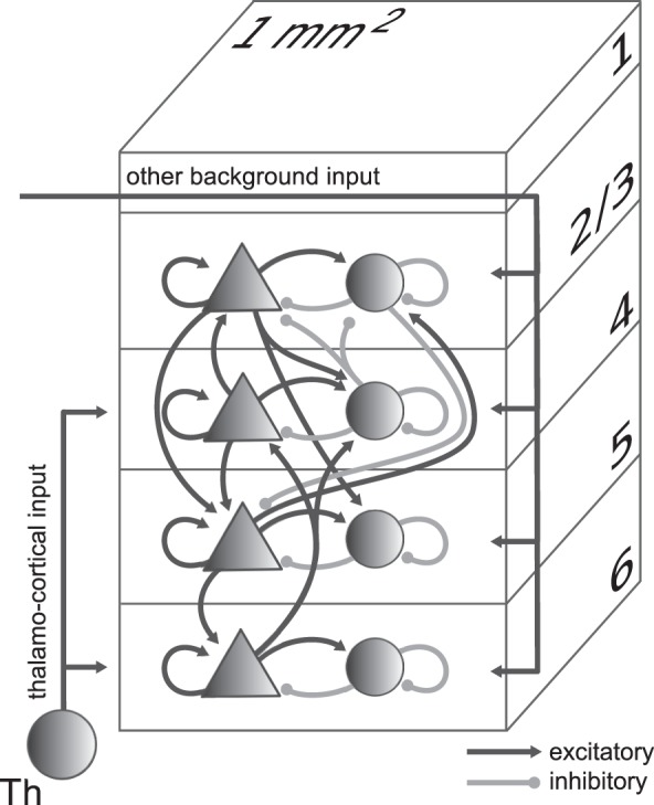
Model definition. Layers 2/3, 4, 5, and 6 are each represented by an excitatory (triangles) and an inhibitory (circles) population of model neurons. The number of neurons in the population is chosen according to Binzegger et al. (2004) based on the countings of Beaulieu and Colonnier (1983) and Gabbott and Somogyi (1986). Input to the populations is represented by thalamo-cortical input targeting layers 4 and 6 and other external background input to all populations. Excitatory (black) and inhibitory (gray) connections with connection probabilities >0.04 are shown. The model size corresponds to the cortical network under a surface of 1 mm2.
Following this balanced random network approach, we employ spiking leaky integrate-and-fire neurons interacting with static synapses, whereby the inhibitory interactions are stronger than excitatory ones to provide a balanced condition. The structural parameters of our multilaminar extension, that is, the connectivity and the external inputs are derived from experimental data. This choice enables us to expose the dynamical consequences of the structure of the local microcircuit in spiking cortical networks unaffected by additional cell-type specificity (e.g. Brémaud et al. 2007; Lefort et al. 2009). The employed connectivity map integrates the 2 major connectivity maps from anatomy (Binzegger et al. 2004) and electrophysiology (Thomson, West, et al. 2002) and furthermore incorporates insights from photostimulation (Dantzker and Callaway 2000; Zarrinpar and Callaway 2006) and electron microscopy (EM, McGuire et al. 1984) studies, which report the specific selection of interneurons by a subset of interlayer projections.
The modeling approach minimizes the number of parameters of the network model and, in combination with the algorithmic integration of the connectivity data, avoids any fitting or tuning of the activity. However, in order to benefit from the insights of a large number of studies, we are forced to combine data from some species and areas, focusing on rat primary visual and somatosensory areas and cat area 17. When new data become available, the presented method for the integration of different experimental approaches may be applied to build more specific models. We find that our integrated connectivity map, with all other parameters constrained as in the balanced random network model (Brunel 2000), yields cell-type specific spontaneous and stimulus-evoked activity in good agreement with experimentally observed activity.
Our study is structured as follows. We first compare the 2 major connectivity maps from anatomy and physiology. The observed consistencies and differences drive the development of the methodology to combine the 2 data sets algorithmically by correcting for the different experimental procedures: We apply a lateral connectivity model and employ available information on the specific selection of target types. Subsequently, we present the resulting integrated connectivity map and analyze its main features. Secondly, we use the integrated map in full-scale spiking network simulations of the cortical microcircuit. We analyze the spontaneous activity, the stimulus-evoked response patterns, and the role of the specific target type selection for the stability and the propagation of activity. Finally, we discuss, based on our findings, the operational principles of the cortical microcircuit and provide an outlook on the relevance of the presented results for future studies.
Materials and Methods
The network model (Fig. 1) represents 4 layers of cortex, L2/3, L4, L5, and L6, each consisting of 2 populations of excitatory (e) and inhibitory (i) neurons. Throughout the paper, we use the term “connection” with reference to populations, defined by the pre- and postsynaptic layers and neuron types. The term “projection” is used for the 2 connections of a single presynaptic population to both populations of a target layer. The “connection probability” of a connection defines the probability that a neuron in the presynaptic population forms at least 1 synapse with a neuron in the postsynaptic population. A “connectivity map” is defined by the 64 connection probabilities between the 8 considered cell types.
Connectivity Data
For the anatomical map (a), Binzegger et al. (2004) use data based on reconstructed neurons that have been filled in vivo with horseradish peroxidase and a modified version of Peters' rule (Braitenberg and Schüz 1998) based on layer-specific distributions of boutons and dendrites. They provide the relative number of synapses participating in a connection and the total absolute number of synapses, depending on the pre- and postsynaptic type, of area 17 (Supplementary Table 1). The product of these measures gives the absolute number of synapses K for any connection. To calculate the corresponding connection probabilities Ca, we assume that the synapses are randomly distributed, allowing for multiple contacts between any 2 neurons. With Npre(post) being the number of neurons in the presynaptic (postsynaptic) population, we obtain:
 |
(1) |
The often used expression
 |
(2) |
is the corresponding first-order Taylor series approximation and valid for small K/(Npre
Npost) (Supplementary Material). The original published data constitute our “raw” connectivity map (Binzegger et al. 2004, their Fig. 12). Consistent with other modeling work (Izhikevich and Edelman 2008), we construct an improved (“modified”) anatomical map by assigning the unassigned symmetric (inhibitory) synapses, originating from a potential underestimation of interneuronal connectivity, to within-layer projections originating from local interneurons (Binzegger et al. 2004). The derived connection probabilities are inversely proportional to the considered surface area πr2 (Fig. 2B). This can be easily understood when considering the approximation eq. (2): The numbers of neurons N and synapses K increase linearly with the surface area and therefore  . The product of the connection probability and the surface area is constant for large areas (Fig. 2B). Hence, we use the area-corrected connection probability
  for all numerical values of the anatomical map throughout this paper.
Figure 2.

Properties of connectivity maps. (A) Connection probabilities according to the anatomical (top panel, circles) and physiological connectivity maps (center panel, squares) and corresponding discrepancy indices (bottom panel, triangles). Both raw (closed markers) and modified (open markers) maps are shown (also provided in Supplementary Table 1). The data are horizontally arranged according to their classification as within-layer (black) and interlayer (gray) connections. For a given pair of pre- and postsynaptic layer, the data are arranged from left to right according to connection types: Excitatory to excitatory, excitatory to inhibitory, inhibitory to excitatory, and inhibitory to inhibitory. L5i to L5e/i outside of the displayed range, see Supplementary Table 1. Error bars are minimal statistical errors (Supplementary Material). (B) Dependence on sampling radius of the anatomical connection probability (solid: eq. (1), dashed: eq. (2)) and the product of connection probability and area (dotted) in double-logarithmic representation. (C) Anatomical and physiological recurrence strength. (D) Anatomical and physiological loop strength. Error bars in C and D are based on the minimal statistical error estimates of connection probabilities using error propagation.
The physiological hit rate estimates (Thomson, West, et al. 2002, their Table 1) provide the physiological map (p). We combine multiple independently measured hit rates for the same connection by a weighted sum:
 |
(3) |
where Ri and Qi are the hit rate and the number of tested pairs in the ith experiment, respectively. In accordance with Haeusler and Maass (2007), we set the probabilities of the L2/3i to L5e and of the L4i to L2/3i connections to 0.2. While these data constitute the raw map, we incorporate additional hit rate estimates (Table 1) to create an improved (“modified”) physiological connectivity map. Thereby, we combine several studies that are partly based on different recording and sampling techniques as listed and thoroughly discussed in Thomson and Lamy (2007). The numerical values of all connectivity maps are listed in Supplementary Table 1.
Table 1.
Modified physiological connectivity map
Notes: The map incorporates the hit rate estimates from a number of studies. The selection of studies is based on the comprehensive review by Thomson and Lamy (2007) including all data where the hit rate and the number of tested pairs can be extracted such that eq. (3) is applicable. The table lists, from left to right, the connection, the number of existing connections (the product of hit rate and number of tested pairs), the number of tested pairs, and the publication from which the data are extracted. The physiological estimate on the L2/3e to L6e connection is estimated from Zarrinpar and Callaway (2006), a photostimulation study reporting a nonzero but low connectivity for this connection. The abbreviations relate to the subtype of interneurons investigated in the respective publication: Fast-spiking (FS), low-threshold spiking (LTS), and somatostatine-positive labeled (SOM) interneurons. Furthermore, we use the following additional data on within-layer connections that are not reported separately: Thomson et al. (1996); Thomson and Lamy (2007): i to e in L2/3, L4, and L5 21 connected of 93 tested pairs; Ali et al. (2007): i to e in L2/3, L4, and L5 30 connected of 90 tested pairs, e to i in L2/3, L4, and L5 21 connected of 48 tested pairs; i to e in L2/3 and L4 9 connected of 69 tested pairs, and e to i in L2/3 and L4 21 connected of 147 tested pairs. The reported numbers of connected and tested pairs are uniformly distributed to the reported layers.
*The number of tested pairs is not explicitly given, but estimated from the stated accuracy of the connection probability.
We classify all connections into 2 main groups: Recurrent intralayer or “within-layer” connections and connections between different layers or “interlayer” connections.
Lateral Connectivity Model
The experimental methods underlying both the anatomical and physiological connectivity maps provide connection probabilities for different cell types in different layers, but sample from different lateral spreads: The anatomical data correspond to a very large cortical surface area, parameterized by the sampling radius ra. This radius is determined by the reconstructed neuronal morphology and the applied analysis working on neuronal and synaptic densities, but not actual neuron morphologies. In contrast, the physiological map is based on paired recordings in slices and thereby on very local data, sampling cells with a rather low maximal lateral distance, rp.
To address the differences originating from the 2 experimental approaches, we use a Gaussian model for describing the lateral connection probability profile:
 |
(4) |
with r being the lateral distance between neurons. The model parameters C0 and σ specify the peak connection probability (zero lateral distance) and the lateral spread of connections, respectively. In this framework, the experimental data correspond to a random sampling of connections within a cylinder of a fixed sampling radius and corresponding mean connection probabilities  , yielding the 2 equations:
 |
(5) |
 |
(6) |
Furthermore, we assume that the underlying lateral connectivity is the same for both maps, that is, C0 and σ are universal. In this way, we can utilize the 2 different experimental approaches, yielding Ca and Cp in equations (5) and (6) with 2 different lateral sampling radii ra and rp to determine the 2 unknown parameters of the lateral connectivity model C0 and σ. We find:
 |
which can be solved numerically for σ. For  , we have
  and therefore
 |
(7) |
and
 |
(8) |
In principle, this approach may be applied to any individual connection between 2 cell types. However, we determine σ and C0 only for the global mean connection probabilities of the 2 maps, providing robustness against uncertainties in the probability estimate of a particular connection.
The lateral connectivity model is exclusively used to reconcile the 2 connectivity maps; the simulations use a laterally uniform connectivity profile, that is, the connectivity between 2 neurons is only determined by the cell types and not their location in space. The mean connection probability of the model Cm depends on the size of the network (e.g. the surface area, ) and the parameters of the lateral model, but by applying equations (7) and (8), this can also be expressed in terms of the experimentally accessible parameters, Cp, rp, and
  :
:
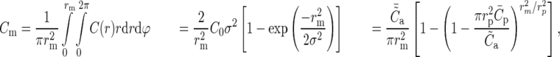 |
(9) |
where  and
and  specify the global means. To arrive at the individual connection probabilities at a given model size, it is sufficient to multiply a connectivity map by the ratio of Cm and the global mean of the map
  .
.
Connectivity Data Analysis
To compare the connectivity maps, we define 2 measures, the “recurrence strength” as the ratio of the mean within-layer and the mean interlayer connection probabilities and the “loop strength” as the ratio of the mean connection probability of the cortical feed-forward loop (Gilbert 1983, L4 to L2/3 to L5 to L6 to L4) and the mean connection probability of all other interlayer connections. For a fair comparison of the 2 maps, we base the recurrence strength and the loop strength measures only on connections for which estimates of within- and interlayer connections are available in both data sets. Therefore, L2/3, L4, and L5 are included in these specific calculations, but not L6.
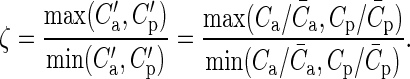
A measure with higher resolution is the discrepancy index ζ, which compares the connection probabilities of individual connections, provided both connectivity maps assign nonzero probabilities. We first remove global differences due to lateral sampling by scaling the maps to the mean model connectivity:  . The discrepancy index is then defined as the ratio of the maximum and the minimum of the scaled maps:
 |
(10) |
The measure is independent of the model connectivity because Cm cancels from the expression. The discrepancy index of individual connections is 1 if the estimates only differed due to the lateral sampling, else it is >1.
Furthermore, to quantify the specificity of connections, we introduce the target specificity
 |
(11) |
as the normalized difference of the connection probabilities constituting a projection.
Consistent Modifications of Target Specificity
To construct a consistent integrated connectivity map, it is necessary to modify the target specificity of certain projections (see Results, Table 2), that is, connection probabilities are modified to meet a given target specificity value. However, we constrain these modifications by demanding consistency with the underlying experimental data. For the anatomical data, this underlying measure is the number of synapses participating in a projection. For the physiological data, in several cases, exclusively the connection to 1 of the 2 neuron types in a target layer has been measured (e.g. for L2/3e to L5 only to excitatory targets). This measurement is conserved, while the experimentally not quantified connection is estimated (in this example L2/3e to L5i).
Table 2.
Amendment candidates for target specificity
| Projection | T | Data source |
|---|---|---|
| L2/3e to L4 | −0.8 | Thomson, West, et al. (2002) |
| L5e to L2/3 | −0.4 | Dantzker and Callaway (2000) |
| L2/3e to L6 | −0.4 | Zarrinpar and Callaway (2006) |
| L6e to L4 | −0.4 | McGuire et al. (1984) |
| L2/3e to L5 | 0.29 | Binzegger et al. (2004) |
| L4e to L5 | 0.32 | Binzegger et al. (2004) |
| L2/3i to L5 | 0.4 | Binzegger et al. (2004) |
| L4i to L2/3 | 0.23 | Binzegger et al. (2004) |
Notes: The rows describe the projections whose target specificities are modified during the compilation of the integrated connectivity map. For each projection, the second column states the target specificity value T after the amendment, the third the publication on which the modification is based. The top 4 rows are the candidate projections for a preference of inhibitory targets. In these cases, no quantitative estimates are known. T = −0.8 is set if the literature provides a strong indication and T = −0.4 for a comparably weak indication (compare Supplementary Material). The T-values of the bottom 4 rows are based on the anatomical map and provide estimates of the previously not measured connections to inhibitory neurons for the physiological map.
Modifying the connection probabilities while conserving the total number of synapses of a projection requires a redistribution of synapses across the target neurons (Supplementary Fig. 1). To that end, we determine from eq. (11) the fraction of synapses targeting excitatory neurons Δ as a function of the requested target specificity and constrained by the total number of synapses and the sizes of the presynaptic and the 2 postsynaptic populations. The main complication is that target specificity in eq. (11) is defined in terms of connection probabilities and the relation of connection probability with the number of synapses is nonlinear, see eq. (1). The exact value of Δ is found by numerically solving:
 |
(12) |
In the first-order Taylor series expansion of C, eq. (2), the relation is linear and, substituting  and
and  in eq. (11), we find:
 |
For a given Δ, we estimate the new connection probabilities by applying eq. (1) with the number of synapses ΔK and (1 − Δ)K for excitatory and inhibitory targets, respectively.
The modifications of the physiological data are straightforward because, in all cases considered here, only one connection probability is experimentally given so that we can estimate the unknown value based on the definition of eq. (11):
 |
(13) |
Compilation of the Integrated Connectivity Map
We compile the integrated connectivity map algorithmically. The procedure requires as input  , that is, the anatomical and the physiological connectivity maps, the physiological sampling radius, the model size, and information about desired modifications of the target specificities. Then, it automatically estimates the mean model connectivity according to the Gaussian lateral connectivity model, eq. (9), scales the connectivity maps to match the mean values, and incorporates the target specificities into both maps. The target specificities are modified separately for the anatomical and the physiological map, as explained in the previous section, equations (12) and (13). After these amendments, the 2 maps are merged by averaging (see also Supplementary Fig. 2 for a technical description).
Layer-Specific External Input
In our simulations, we study spontaneous and stimulus-evoked activity. In both cases, the external, or “background”, inputs are activated. The transient stimulation consists of an increase in the firing rate of thalamic relay cells. To parameterize the model, we estimate the number of inputs that a neuron of a given cell type receives from the experimental data.
We distinguish between 3 types of inputs to the local cortical network: Thalamic afferents, “gray matter” external inputs, that is, intrinsic nonlocal inputs entering the local network through the gray matter, and other “white matter” external inputs, which include all inputs not covered by the previous types. The thalamic afferents (of type X and Y) are included in the anatomical connectivity map (Binzegger et al. 2004). We extract the gray matter inputs from the information on bouton distributions in 3-dimensional space described in Binzegger et al. (2007). The authors find that boutons of all cell types form multiple clusters and the article provides the lateral distance between cluster centers and the corresponding somata. We interpret a cluster to be nonlocal if the lateral distance to the soma is greater than approximately 0.56 mm (corresponding to a local network surface area of 1 mm2). By additionally using data on the relative sizes of different cluster types, we estimate the proportion of intrinsic gray matter connections that originate outside of the local network. Thereupon, we use the estimated proportion of gray matter inputs and the number of local connections in our network to calculate the absolute number of gray matter inputs. In this way, we construct an estimate of the gray matter external inputs which is consistent with both the axonal structure in Binzegger et al. (2007) and the structure of our model. The detailed procedure is described in Supplementary Material (Section 3 and Supplementary Table 2).
The white matter inputs are estimated based on the comparison of the absolute number of synapses obtained in Binzegger et al. (2004), which only contains the contributions from local, thalamic, and gray matter synapses, with those in Beaulieu and Colonnier (1985) containing all synapses. The difference has been termed the “dark matter” of cortex (Binzegger et al. 2004) and, in case of the excitatory synapses, is usually interpreted as white matter external inputs. The explicit numbers are published in Izhikevich and Edelman (2008, their Fig. 9 of the Supplementary Material) at subcellular resolution. As our model is based on point neurons, we sum over all contributions to a given cell type and average across the cell types that are collapsed to a single population. Thereby, our estimates take neuronal morphology into account.
The resulting counts for the 3 external input types and the total number of external inputs to the excitatory populations are given in Table 3. Since long-range projections target excitatory and inhibitory neurons (Johnson and Burkhalter 1996; Gonchar and Burkhalter 2003), we choose target specificity values for external inputs to be comparable with recurrent connections, resulting in similar total numbers of external inputs to inhibitory neurons (Table 5).
Table 3.
Layer-specific external inputs
| External inputs | L2/3 | L4 | L5 | L6 |
|---|---|---|---|---|
| Thalamic | 0 | 93 | 0 | 47 |
| Gray matter | 534 | 353 | 389 | 79 |
| Other white matter | 1072 | 1665 | 1609 | 2790 |
| Total | 1606 | 2111 | 1997 | 2915 |
Notes: From top to bottom, the estimated numbers of external inputs per neuron are shown for excitatory neurons in layers 2/3, 4, 5, and 6 for the 3 distinguished input types: Thalamic, gray matter, and other white matter inputs. The total number of external inputs is rounded for simulations (compare Table 4).
Table 5.
Parameter specification
|
Populations and inputs | ||||||||||
|---|---|---|---|---|---|---|---|---|---|---|
| Name | L2/3e | L2/3i | L4e | L4i | L5e | L5i | L6e | L6i | Th | |
| Population size, N | 20 683 | 5834 | 21 915 | 5479 | 4850 | 1065 | 14 395 | 2948 | 902 | |
| External inputs, kext (reference) | 1600 | 1500 | 2100 | 1900 | 2000 | 1900 | 2900 | 2100 | n/a | |
| External inputs, kext (layer independent) | 2000 | 1850 | 2000 | 1850 | 2000 | 1850 | 2000 | 1850 | n/a | |
| Background rate, νbg | 8 Hz | |||||||||
| Connectivity | ||||||||||
| from | ||||||||||
| L2/3e | L2/3i | L4e | L4i | L5e | L5i | L6e | L6i | Th | ||
| to | L2/3e | 0.101 | 0.169 | 0.044 | 0.082 | 0.032 | 0.0 | 0.008 | 0.0 | 0.0 |
| L2/3i | 0.135 | 0.137 | 0.032 | 0.052 | 0.075 | 0.0 | 0.004 | 0.0 | 0.0 | |
| L4e | 0.008 | 0.006 | 0.050 | 0.135 | 0.007 | 0.0003 | 0.045 | 0.0 | 0.0983 | |
| L4i | 0.069 | 0.003 | 0.079 | 0.160 | 0.003 | 0.0 | 0.106 | 0.0 | 0.0619 | |
| L5e | 0.100 | 0.062 | 0.051 | 0.006 | 0.083 | 0.373 | 0.020 | 0.0 | 0.0 | |
| L5i | 0.055 | 0.027 | 0.026 | 0.002 | 0.060 | 0.316 | 0.009 | 0.0 | 0.0 | |
| L6e | 0.016 | 0.007 | 0.021 | 0.017 | 0.057 | 0.020 | 0.040 | 0.225 | 0.0512 | |
| L6i | 0.036 | 0.001 | 0.003 | 0.001 | 0.028 | 0.008 | 0.066 | 0.144 | 0.0196 | |
| Name | Value | Description | ||||||||
| w ± δw | 87.8 ± 8.8 pA | Excitatory synaptic strengths | ||||||||
| g | –4 | Relative inhibitory synaptic strength | ||||||||
| de ± δde | 1.5 ± 0.75 ms | Excitatory synaptic transmission delays | ||||||||
| di ± δdi | 0.8 ± 0.4 ms | Inhibitory synaptic transmission delays | ||||||||
| Neuron model | ||||||||||
| Name | Value | Description | ||||||||
| τm | 10 ms | Membrane time constant | ||||||||
| τref | 2 ms | Absolute refractory period | ||||||||
| τsyn | 0.5 ms | Postsynaptic current time constant | ||||||||
| Cm | 250 pF | Membrane capacity | ||||||||
| Vreset | −65 mV | Reset potential | ||||||||
| θ | −50 mV | Fixed firing threshold | ||||||||
| νth | 15 Hz | Thalamic firing rate during input period | ||||||||
The categories refer to the model description in Table 4.
The described procedure yields the reference parameterization of the cell-type specific external inputs (simulation results shown in Fig. 6). However, the data basis is limited and the effect of the input parameterization on the model has to be investigated. Therefore, we compare our results with various simulations with different background inputs. At first, the Poissonian background spikes are substituted by a direct current (DC) input (Fig. 7A). Secondly, the firing rate per background synapse is modified (compare Fig. 8). Thirdly, we investigate the role of different numbers of input synapses per neuron. To this end, we compare our reference with a layer-independent parameterization where the number of inputs to each layer is identical (Table 5 and Fig. 7B). In addition, we conduct a series of 100 simulations where we choose the inputs to our simulation at random within specific intervals (Fig. 7C): For each layer (e.g. L2/3), we first determine the number of inputs to the excitatory population by randomly choosing a number from the range between the value of the reference and the layer-independent parameterization (for L2/3e between 1600 and 2000, e.g. 1870 is drawn). Subsequently, the number of inputs to the respective inhibitory population is chosen conditional on the previous drawing such that the target specificity of the external input to a given layer is between 0 and 0.1 (for the above L2/3 example, this would imply a number between the value for L2/3e, 1870 and the value corresponding to a target specificity of 0.1, 1530, e.g., 1610 is drawn). Due to the higher number of inputs to L6e, we allow for a wider range of target specificity values and the input to L6i is selected to realize a target specificity between 0 and 0.2.
Figure 6.
Simulated spontaneous cell-type specific activity. (A) Raster plot of spiking activity recorded for 400 ms of biological time of layers 2/3, 4, 5, and 6 (from top to bottom; black: Excitatory, gray: Inhibitory). Relative number of displayed spike trains corresponds to the relative number of neurons in the network (total of 1862 shown). (B–D) Statistics of the spiking activity of all 8 populations in the network based on 1000 spike trains recorded for 60 s (B and C) and 5 s (D) for every population. (B) Boxplot (Tukey 1977) of single-unit firing rates. Crosses show outliers, stars indicate the mean firing rate of the population. (C) Irregularity of single-unit spike trains quantified by the coefficient of variation of the interspike intervals. (D) Synchrony of multiunit spiking activity quantified by the variance of the spike count histogram (bin width 3 ms) divided by its mean.
Figure 7.

Dependence of spontaneous activity on input. (A1–A2) Spontaneous activity after replacing the Poissonian background spikes with DC currents. Cell-type specific external input currents equivalent to the reference parameterization for the number of inputs. (A1) Raster plot shows spiking activity recorded for 500 ms of biological time of layers 2/3, 4, 5, and 6 (from top to bottom; black: Excitatory, gray: Inhibitory). Relative number of displayed spike trains corresponds to the relative number of neurons in the network (total of 1862 shown). (A2) Average firing rates of the spiking activity shown in A1. (B1–B2) Spontaneous activity with layer-independent Poissonian background inputs (Table 5). Raster plot (B1) and firing rate histogram (B2) equivalent to A1 and A2. (C) Histograms of the excitatory and inhibitory population firing rates for L2/3 (C1), L4 (C2), L5 (C3), and L6 (C4) for randomly drawn external inputs (100 trials, see Materials and Methods for details).
Figure 8.
Dependence of network activity on the external background firing rate and the relative inhibitory synaptic strength. White stars mark the reference parameter set. (A) Population firing rates of excitatory populations in layers 2/3 (squares), 4 (diamonds), 5 (circles), and 6 (triangles), lightness increases with cortical depth, as a function of the background rate at fixed relative inhibitory synaptic strength (g = 4). (B) AIness%, the percentage of populations with the firing rate <30 Hz, irregularity between 0.7 and 1.2, and synchrony <8 (data collected for 5 s per simulation), as a function of the background rate and the relative inhibitory synaptic strength. Labeled black contour lines indicate areas where 50%, 75%, and 100% of all populations fire asynchronously and irregularly at low rate. Dashed contour lines confine the area where the firing rates are ordered in accordance to Table 6. (C) Population firing rates of excitatory populations as a function of the relative inhibitory synaptic strength at fixed background rate (8 Hz) (markers as in A).
To simulate stimulus-evoked activity, we explicitly model the thalamic input to L4 and L6 by a thalamic population of 902 neurons (Peters and Payne 1993). These relay cells emit Poissonian spike trains at a given rate in some prescribed time interval and are randomly connected to the cortex with the cell-type specific connection probabilities according to Binzegger et al. (2004); see Table 5. As the number of thalamic inputs is also included in the background input, this set-up corresponds to an increase in thalamic firing rates. Here, we present results based on a firing rate increase of 15 Hz that lasts 10 ms.
Network Simulations
The simulations are full scale in the sense that they comprise the same number of neurons and synapses as found in the local cortical microcircuit where locality is defined by the average lateral range of local connectivity (Fig. 3). Correspondingly, the model consists of about 80 000 neurons and 0.3 billion synapses. The network is defined by 8 neuronal populations representing the excitatory and inhibitory cells in L2/3, L4, L5, and L6. The populations consist of current-based leaky integrate-and-fire model neurons with exponential synaptic currents and are randomly connected with connection probabilities according to the integrated connectivity map we derive in this article. Every population receives Poissonian background spike trains (Amit and Brunel 1997; Brunel 2000); the firing rates of these inputs are determined by the number of external inputs a neuron in a particular population receives and the background spike rate contributed by each synapse. Synaptic strengths and synaptic time constants of all connections are chosen such that an average excitatory postsynaptic potential has an amplitude of 0.15 mV with a rise time of 1.6 ms and a width of 8.8 ms mimicking the in vivo situation (Fetz et al. 1991). Inhibitory postsynaptic potentials are negative and increased by a factor g compared with the excitatory ones. The synaptic strengths of the excitatory to excitatory connection from L4 to L2/3 are doubled as the data basis for these connections is not fully conclusive (Supplementary Fig. 7). Delays in the network are chosen independent of the layer, with excitatory delays being on average around twice as long as inhibitory delays (based on differences in conduction delays discussed in Thomson and Bannister (2003)), but the exact ratio is uncritical. To introduce heterogeneity into the network, we draw the synaptic strengths and delays from Gaussian distributions (prohibiting a change of sign of the strengths and constricting delays to be positive and multiples of the computation step size). We simulated various settings of the synaptic parameters (strengths and delays) without striking impact on the results. The network structure and a complete list of parameters as well as their values in the reference network model are systematically described according to Nordlie et al. (2009) in Tables 4 and 5.
Figure 3.
Lateral connectivity model. (A) Two-dimensional Gaussian with 2 cylinders indicating the lateral sampling of the anatomical (gray outer cylinder) and the physiological (black inner cylinder) experiments. (B) Estimated peak amplitude C0 and (C) lateral spread σ of the connectivity model based on mean connectivity of the anatomical and physiological raw and modified maps. (D) Average connection probability (black line, based on eq. (9)) and (E) average synaptic convergence (black line, average number of synaptic inputs per neuron derived from the connection probability and the number of neurons using eq. (1)) of the layered network model as a function of the network size expressed in number of neurons. The dashed horizontal line marks 85% of the maximal synaptic convergence in the local network. Black diamonds show the data used in our simulations, further markers indicate other published cortical network models: Haeusler and Maass (2007) (light gray square), Izhikevich (2006) (light gray triangle), Izhikevich et al. (2004) (light gray circle, embedded local network is defined by the area receiving connections from a single long-range axon), Lundqvist et al. (2006); Djurfeldt et al. (2008) (light gray diamond, local network represented by one hypercolumn), Vogels and Abbott (2005); Vogels et al. (2005) (dark gray circle), Sussillo et al. (2007) (dark gray square), Brunel (2000) (dark gray triangle), Kriener et al. (2008) (dark gray diamond), Kumar et al. (2008) (black circles), and Morrison et al. (2007) (black square).
Table 4.
Model description after Nordlie et al. (2009)
|
Model summary | |
|---|---|
| Populations | Nine; 8 cortical populations and 1 thalamic population |
| Topology | — |
| Connectivity | Random connections |
| Neuron model | Cortex: Leaky integrate-and-fire, fixed voltage threshold, fixed absolute refractory period (voltage clamp), thalamus: Fixed-rate Poisson |
| Synapse model | Exponential-shaped postsynaptic currents |
| Plasticity | — |
| Input | Cortex: Independent fixed-rate Poisson spike trains |
| Measurements | Spike activity, membrane potentials |
| Populations | |
| Type | Elements |
| Cortical network | iaf neurons, 8 populations (2 per layer), type specific size N |
| Th | Poisson, 1 population, size Nth |
| Connectivity | |
| Type | Random connections with independently chosen pre- and postsynaptic neurons; see Table 5 for probabilities |
| Weights | Fixed, drawn from Gaussian distribution |
| Delays | Fixed, drawn from Gaussian distribution multiples of computation stepsize |
| Neuron and synapse model | |
| Name | iaf neuron |
| Type | Leaky integrate-and-fire, exponential-shaped synaptic current inputs |
| Subthreshold dynamics | 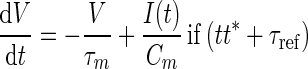 |
| V(t) = Vreset else | |
 |
|
| Spiking | If 
|
| 1. set t* = t, 2. emit spike with time stamp t* | |
| Input | |
| Type | Description |
| Background | Independent Poisson spikes to iaf neurons (Table 5) |
| Measurements | |
| Spiking activity and membrane potentials from a subset of neurons in every population | |
To instantiate the network model, we randomly draw for every synapse the pre- and the postsynaptic neuron. In contrast to the often used convergent and divergent connectivity schemes (Eppler et al. 2009), this procedure results in binomially distributed numbers of incoming and outgoing synapses. In practice, we could first calculate the total number of synapses forming a connection by inverting eq. (1) and then successively create the synapses. In a distributed simulation set-up, however, this procedure is inefficient because the neurons are distributed over multiple processes. Although a synapse is only created if the postsynaptic neuron is local to the process (Morrison et al. 2005), the full algorithm would have to be carried out on each process. We solve this problem by calculating a priori how many synapses will be created locally on each process, exploiting that the distribution of synapses over processes is multinomial. Subsequently, we apply the serial algorithm on every machine to the local synapses only: The presynaptic neuron is drawn from all neurons in the presynaptic population and the postsynaptic cell on a given process is drawn only from the neurons located on this process (compare Supplementary Fig. 6). While the first step is serial, but efficient for the number of processes we typically employ, the second step is fully parallelized. The procedure is detailed in the Supplementary Material.
All simulations are carried out with the NEST simulation tool (Gewaltig and Diesmann 2007) using a grid constrained solver and a computation step size h = 0.1 ms on a compute cluster with 24 nodes each equipped with 2 quad core AMD Opteron 2834 processors and interconnected by a 24-port Voltaire InfiniBand switch ISR9024D-M. Forty-eight cores simulate the network of around 80 000 neurons and 0.3 billion synapses in close to real time (Djurfeldt et al. 2010). A reference implementation of the wiring algorithm (RandomPopulationConnect) and an implementation of the network simulation will be made available with the next release of the NEST simulation tool (http://www.nest-initiative.org).
Results
Comparison of Connectivity Maps
The anatomical and the physiological connectivity maps are shown in Figure 2. We observe that the estimated absolute connection probabilities are different for both maps, but exhibit a similar structure: Recurrent within-layer connections are all nonzero with the densest connectivity in superficial layers. Interlayer connections can be subdivided into connections with probabilities of the same order of magnitude as within-layer connections and those with values close or equal to zero. These observations hold for the raw data and for the modified data.
We quantify the relation of the 2 connectivity maps by several measures (as defined in section Materials and Methods). First, we determine the relative connectivity of subsets of the connectivity maps: The recurrence strength compares within-layer and interlayer connectivity (Fig. 2C) and the loop strength the average connectivity of the feed-forward loop and other interlayer connections (Fig. 2D). We find that both measures are statistically indistinguishable for the 2 maps (z-test, P > 0.1 and 0.05, respectively), highlighting the overall similarity of both maps. Secondly, we compare the individual connections by the discrepancy index (Fig. 2A, lower panel). This measure reveals that particularly interlayer connections are partly not consistently estimated: 50% of the discrepancy indices of interlayer connections are large (L2/3e to L4i, L5e to L2/3e, L4i to L2/3e, and L4i to L2/3i) for both the raw and the modified data.
In the following, we first exploit the overall similarity of relative connectivity measures between the 2 maps in a lateral connectivity model and then address the different estimates of a subset of interlayer connections by means of the target specificity of connections.
Lateral Connectivity
We hypothesize that the differences in the mean connection probabilities are explained by differences in the methodology applied to obtain the connectivity maps: Physiological recordings in slices are usually restricted to a maximal lateral distance of the somata of around 100 μm (as reported in Thomson and Morris (2002) for the raw physiological map). The anatomical data, in contrast, are based on reconstructed axons and dendrites, with axons extending up to 4 mm (Binzegger et al. 2007), in general beyond 1 mm. When providing absolute numbers, Binzegger et al. (2004) refer to the surface area of cat area 17 (399 mm2).
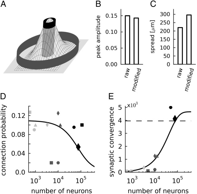
We exploit the information on the experimental methods to account for the different experimental sampling radii (for details see Materials and Methods) by evaluation of a Gaussian lateral connectivity model (eq. 4) similar to the one by Hellwig (2000) and Buzas et al. (2006). We assume the model to reflect the in vivo connectivity structure and the experimental connectivity maps to characterize samples of this structure. The anatomical measurement is interpreted as an unconstrained sampling over the complete lateral connectivity structure, whereas the physiological measurement corresponds to a local measure sampling from the center region of the Gaussian.
The model's 2 parameters, peak connection probability, and lateral spread are determined based on the mean connection probabilities of the 2 maps and the physiological sampling radius (equations 7 and 8). Figure 3A illustrates the approach to determine the 2 parameters by the 2 independent measurements of mean values and Figure 3B,C provides the estimates based on the raw and modified connectivity maps, respectively. One experimental parameter, the physiological sampling radius, is only reliably provided for the raw data set (100 μm, Thomson and Morris 2002). We apply the same value to the modified physiological map. A sensitivity analysis (data not shown) shows that a larger sampling radius implies an increased zero-distance connection probability and a decreased lateral spread and that the effect is small: The estimates of both parameters change by <8% when altering the sampling radius from 50 to 150 μm.
The estimated lateral spread is consistent with data from rat and cat primary visual cortex, which were obtained based on morphological reconstructions and the potential connectivity method: Hellwig (2000, his Fig. 7), reports a lateral spread of 150–310 μm, and Stepanyants et al. (2008, their Fig. 7), find a spread of around 200 μm of main projections in input and output maps. Also, the overall connectivity level of 0.138 for nearby neurons with a distance of 100 μm is in good agreement with the extensively used estimate of 0.1 provided by Braitenberg and Schüz (1998). These consistencies indicate that our underlying assumption—anatomical and physiological experiments sample independently from the same lateral connectivity profile—is valid.
Average Model Connectivity
We use the Gaussian lateral connectivity model exclusively to determine the average connection probability of a pair of neurons at a given network size (Fig. 3D). Thus, the network model consists of randomly connected populations; the neurons do not exhibit a lateral connectivity profile. The connectivity of small networks (up to about 7000 neurons) is largely determined by the physiological connectivity and that of large networks (above 100 000 neurons) by the anatomical connection probability (decaying quadratically, see Fig. 2B). For intermediate network sizes, eq. (9) interpolates between these 2 extremes according to the Gaussian lateral connectivity profile. Figure 3E shows the average synaptic convergence as a function of the network size. It reveals, that only sufficiently large network models represent the majority of local synapses: For example, a network of around 80 000 neurons comprises >85% of all local synapses. In contrast, a network consisting of 10 000 neurons represents only around 20% of the local connectivity. Therefore, we select our network to correspond to 1 mm2 of cortical surface (77 169 neurons).
According to our analysis, the maximal average number of local synapses per neuron is about 5000. This number is consistent with the data of Binzegger et al. (2004, see their Fig. 11A). In Figure 3, we also display the connectivities and convergences of a selection of other modeling studies on the local cortical network (some data representing local networks embedded in larger networks). Independent of the model size, most studies use a connection probability of around 0.1, which is largely consistent with our results. Only for large networks of 50 000 neurons and more, this connection probability is above our estimate. Two studies use a significantly smaller connection probability of 0.02, arguing that this value interpolates between high local and low distal connectivity. Although the absolute number differs from our estimate, the reasoning is the same as for our model. In all but 2 cases (Morrison et al. 2007; Kumar et al. 2008), the models' convergence is <20% of the anatomical estimate.
Randomness and Specificity
A central assumption of the anatomical connectivity map is randomness, that is, synapses are established independent of the excitatory or inhibitory nature of the pre- and postsynaptic cells. Nevertheless, the target specificity estimates of the anatomical connectivity map (circles in Fig. 4) are >0.2, reflecting a preferential selection of excitatory targets. The bias is introduced by the application of the modified version of Peters' rule: Binzegger et al. (2004) assume that synaptic densities on dendrites are independent of the cell type and apply this rule to bouton densities and dendritic lengths. The bias to positive target specificity estimates indicates that dendrites of excitatory cells in their data set are generally longer than that of inhibitory cells. Furthermore, some projections exhibit very high values >0.5, because primarily the dendrites of excitatory cells reach into the cloud of presynaptic axonal elements. This rule differs from the formulation by Braitenberg and Schüz (1998), which considers selection of targets on the level of cells not dendrites and by definition yields target specificity values of 0.
Figure 4.
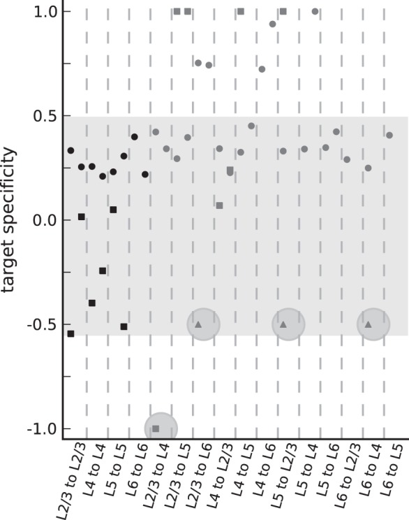
Anatomical (circles) and physiological (squares) estimates of target specificity based on the modified connectivity maps. +1(−1) indicates exclusive selection of excitatory (inhibitory) targets, and 0 random selection. Triangles show additional candidates of inhibition-specific projections discovered in photostimulation or EM studies. The shaded area highlights the estimates of all within-layer projections and the interlayer projections with target specificity values between 0 and 0.5 (“nonspecific” interlayer connections). Within these bounds, the anatomical and physiological estimates are 0.32 ± 0.07 and −0.17 ± 0.28, respectively. The largest statistically well constrained values from a single laboratory are exhibited by the projections L2/3e to L2/3, L4e to L4, and L5e to L5 (compare Supplementary Table 1) of the raw physiological map. The target specificity of these data is −0.01 ± 0.03. The 4 highlighted data points are candidates of specific target type selection. For every pair of pre- and postsynaptic layer, the figure shows data for both presynaptic neuron types (left: Excitatory, right: Inhibitory).
The target specificity values of the physiological map contrast with the anatomical findings. Most values (squares in Fig. 4) are consistently smaller and show larger variability than the anatomical estimates. Excitatory within-layer connections of the raw connectivity map based on Thomson, West, et al. 2002 univocally select their targets independent of the postsynaptic type. Overall, physiological within-layer connections are biased toward negative target specificity values. Several projections in the physiological map, however, connect exclusively to excitatory neurons due to incomplete sampling of or missing experiments on inhibitory subtypes. This highlights that a straightforward application of the currently available physiological connectivity map in simulations results in artifacts due to missing feed-forward inhibition.
The projection from L2/3e to L4 specifically targets inhibitory, but not excitatory cells (see also Table 1). This specific target type selection cannot be explained by differences in the overlap of the excitatory and inhibitory dendrites with the excitatory axons and is therefore beyond the scope of anatomical studies relying on the statistics of neuronal morphology, such as Peters' rule (Binzegger et al. 2004), and also potential connectivity (Stepanyants et al. 2008). The specificity in the interlayer circuitry explains the large discrepancy index of this projection (Fig. 2A).
We identify 3 additional candidates of specific target type selection: L5e to L2/3, L2/3e to L6, and L6e to L4. The projection from L5e to L2/3 is identified based on a photostimulation study that revealed preferred targeting of interneurons (Dantzker and Callaway 2000). In addition, a much higher connectivity has been observed in paired recordings for the connection from L2/3e to L5e than for the inverse connection (Thomson and Bannister 1998; Thomson, West, et al. 2002; Lefort et al. 2009), although axonal arborizations of L5e neurons exist in L2/3 that give rise to a comparable anatomical estimate of the connectivity (e.g. Martin and Whitteridge 1984; Binzegger et al. 2004; Stepanyants et al. 2009). Furthermore, the projection from L2/3e to L6 is identified based on photostimulation experiments (Zarrinpar and Callaway 2006) and that from L6e to L4 based on an EM study (McGuire et al. 1984). The Supplementary Material, Section 2, contains a detailed discussion regarding the selection of these candidates exhibiting specific target type selection. Evidence is not based on comprehensive sampling in paired recordings and remains indicative. We tentatively assume for these projections a lower specificity than for the L2/3e to L4 projection (triangles in Fig. 4). Two of these projections (L2/3e to L4 and L5e to L2/3) are inverse to the feed-forward loop. Thomson and Morris (2002) and Thomson, Bannister, et al. (2002) argued that the specific target type selection plays a distinct functional role, because the inhibition-specific (“i-specific”) feedback projections may prevent reverberant excitation involving L2/3, L4, and L5 and enhance the propagation of synchronous thalamic inputs.
We utilize the information on i-specific feedback and the anatomical estimates to remove for some projections the methodological biases by consistently modifying the respective target specificities (see Materials and Methods and Table 2). Thereby, we estimate previously not measured physiological connection probabilities and introduce the specific selection of targets into the anatomical map. The latter constitutes an effective redistribution of synapses and corresponds to a refinement of Peter's rule (Supplementary Fig. 1).
Integrated Connectivity Map
Based on the information gathered in the previous sections, we now compile an integrated connectivity map. Our proposed algorithmic compilation method is derived from the analysis and comparison of the anatomical and physiological maps. It consists of 4 steps (see Materials and Methods and Supplementary Fig. 2): The procedure 1) collects the input parameters, 2) applies the lateral model to account for the differences in the lateral sampling of the anatomical and physiological experimental methods, 3) corrects for methodological shortcomings expressed in the target specificity of projections (Table 2) by incorporating photostimulation and EM data, and 4) combines the 2 enhanced connectivity maps.
The resulting connection probabilities are given in Table 5 (compare also upper panel of Supplementary Fig. 3 for a representation equivalent to Fig. 2A). For a consistency check, we calculate the discrepancy indices based on our integrated map and the recently published data for excitatory to excitatory connections of the mouse C2 barrel column (Lefort et al. 2009). In this comparison, we combine the data of Lefort et al. (2009) on L2 and L3 to L2/3 and on L5A and L5B to L5 according to eq. (3). The discrepancy indices are low, indicating a good agreement of the connectivity maps (Supplementary Fig. 3, center panel). The main outlier is the recurrent L4e to L4e connection, which exhibits the highest connection probability in the study of Lefort et al. (2009), but rather low values in the physiological and particularly the anatomical map. The target specificity structure of the integrated map (lower panel of Supplementary Fig. 3) reflects rather random selection of targets for within-layer projections, whereas interlayer projections inherit mostly the properties of the anatomical map, except for the 4 candidate i-specific projections.
The cell-type specific convergences and divergences (Fig. 5) show that the integrated connectivity map reflects prominent features of local cortical connectivity: Except for L5e, convergence is dominated by within-layer connections (consistent with, e.g. Douglas and Martin 1991, 2004). Furthermore, the strongest interlayer excitatory to excitatory divergences correspond to the feed-forward loop from L4 to L2/3 to L5 to L6 and back to L4 (Gilbert 1983; Gilbert and Wiesel 1983). The excitatory to inhibitory divergence is dominated by the i-specific feedback connections.
Figure 5.

Cell-type specific convergence (A) and divergence (B) of the integrated connectivity map. The histograms display blocks of data for the 4 different connection types between excitatory (e) and inhibitory (i) neurons (as indicated). For a neuron in the layer specified on the horizontal axis, the individual bar segments show the absolute number of synapses the neuron receives from a source layer (convergence) or establishes in a target layer (divergence). Bar segments are arranged according to the physical location of the layers in the cortex (from top to bottom: L2/3, L4, L5, L6). Hatched bars represent within-layer connections. Lightness of gray increases from superficial to deeper layers. Gray horizontal lines indicate the convergence and divergence of a balanced random network with the same total number of neurons and synapses as the layered model.
By comparing the average convergence and divergence with the neuronal densities of the different cell populations (Supplementary Fig. 4), we find that neurons in the local microcircuit sample most excitatory inputs from L2/3 and fewest from L5 and L6. In contrast, local outputs within the microcircuit project preferentially to L5.
External Inputs
The model consists totally of about 217 million excitatory and 82 million inhibitory synapses. The inhibitory synapse count (64 ± 21 million) is consistent with Beaulieu and Colonnier (1985), while the number of excitatory synapses is lower than their estimate (339 ± 43 million), presumably reflecting that a fraction of all excitatory synapses originates outside of the local network. The ratio of local synapses (total number of synapses in our network model) and all synapses (according to the countings of Beaulieu and Colonnier (1985)) is 0.74, similar to the ratio reported by Binzegger et al. (2004), but see Stepanyants et al. (2009) for a different approach. The number can be related to the ratio of total axonal length per volume originating from local pyramidal cells, which Schüz et al. (2006) estimate to be 55–70%. Including the axons from the inhibitory neurons, the value can be expected to be even closer to our estimate.
Here, we distinguish between thalamic afferents, gray matter, and other white matter inputs to the local network (see Materials and Methods). The resulting total number of external inputs per neuron (Table 3) is lowest in L2/3, intermediate in L4 and L5, and highest in L6. The number of white matter inputs increases with cortical depth, whereas gray matter long-range inputs form most synapses on L2/3 neurons and fewest in L6. Given the presently available data, we cannot exclude that some synapses treated here as the external input actually represent a pathway in the local microcircuit still awaiting comprehensive experimental assessment.
Spontaneous Layer-Specific Activity
Hitherto, we were exclusively concerned with the analysis of the connectivity structure of the local cortical network and the compilation of an integrated connectivity map. Equipped with this, we now turn to full-scale simulations of the local cortical network (see Materials and Methods and Table 4 for a complete description of the network model).
The simulated spontaneous spiking activity of all cell types corresponds, without any additional tuning, to the AI activity state observed in mono-layered balanced random network models (Amit and Brunel 1997; Brunel 2000). Figure 6A–D shows the ongoing spontaneous spiking activity of all populations and the corresponding firing rates, irregularity, and synchrony. The activity varies significantly across cell types. L2/3e and L6e exhibit the lowest firing rates with a mean below or close to 1 Hz. L4e cells fire more rapidly at around 4 Hz and L5e cells at more than 7 Hz. In all layers, inhibitory firing exceeds excitatory rates. The boxplots furthermore visualize that the firing rates of single neurons can substantially differ. For instance in L2/3e, several neurons fire at more than 5 Hz, while the majority of neurons is rather quiescent emitting less than one spike per second. This effect is due to the random connectivity which results in binomially distributed convergences.
Single-unit activity is irregular; the mean of the single unit coefficients of variation of the interspike intervals is >0.8. The population activity is largely asynchronous, but exhibits fast oscillations with low amplitude similar to balanced random networks (e.g. Brunel 2000). We assess the synchrony of every population's multiunit activity by the variability of the spike count histogram (Fig. 6D). At the given firing rates and bin width, the synchrony of the spiking activity is highest in L5e and lowest in L6. The synchrony of the membrane potential traces (Golomb 2007, Supplementary Fig. 8) confirms that the activity is asynchronous.
Dependence on External Inputs
The observed activity features of the network are robust to changes in the specific structure of the external inputs: Replacing the Poissonian background by a constant DC current to all neurons (Fig. 7A) or applying layer-independent Poissonian background inputs (Fig. 7B) yields similar results. In the latter case, the strongly reduced number of inputs to L6e results in a zero L6e firing rate, indicating that the layer-specific input structure (Table 3) is realistic.
We additionally simulate 100 trials with varying numbers of external inputs (randomly drawn constrained by the reference and the layer-independent parameterization, see Materials and Methods), further confirming the previous findings. Figure 7C shows the histograms of the population firing rates in the different layers for excitatory and inhibitory cells. The distribution of excitatory population firing rates in L2/3 and L6 are persistently low. L5e activity exhibits the highest firing rates and also the largest variability. L4e and the inhibitory populations vary only slightly with mean firing rates similar to the reference parameterization (Fig. 6B). The different applied inputs represent a robustness check of the network dynamics against uncertainties in the data and can also be interpreted as different situations in the awake state, for example, biased toward top-down versus bottom-up inputs. Apparently, the local microcircuitry reconfigures the firing rate distributions for different input situations while conserving general features like the low rate regime in L2/3e and L6e. In 85% of the simulations, L2/3e and L6e fire at a lower rate than L4e and simultaneously L5e exhibits the highest firing rate. We also observe the inhibitory firing rate within a given layer to be higher than the excitatory rate in 83% of all cases.
Comparison to In Vivo Activity
Table 6 contrasts the experimentally observed firing rates in individual layers with our simulation results. Experimentally, the spontaneous activity of L2/3e pyramids has been extensively studied. Consistent over species, areas, and behavioral states, the firing rate is <1 Hz, in good quantitative agreement with the model. The L6e firing rates are similar to the model values, although the experimental data base is more sparse. The L4e and L5e firing rates of rat primary somatosensory cortex are lower than in the model, and L5e consistently shows the highest spontaneous activity, also in rat auditory cortex. The activity of cortico-tectal cells in L5 (and L4) of various cortices in the rabbit is slightly higher.
Table 6.
Experimentally measured (awake state) and simulated cell-type specific firing rates
| Species | Area | Firing rates (Hz) |
Data source | |||
|---|---|---|---|---|---|---|
| L2/3e | L4e | L5e | L6e | |||
| Mouse | S1 | 0.61 | — | — | — | Crochet and Petersen (2006) |
| Poulet and Petersen (2008) | ||||||
| Rat | V1 | 0.44 | — | — | — | Greenberg et al. (2008) |
| Rat | M1 | 0.36 | — | — | — | Lee et al. (2006) |
| Rat | S1 | 0.3 | 1.4 | 2–3 | 0.5 | de Kock and Sakmann (2009) |
| Rat | A1 | <1 | — | 3–4 | — | Sakata and Harris (2009) |
| Rabbit | Four areas | <1 | — | 4–7 | <1 | Swadlow (1988, 1989, 1991, 1994) |
| Model | Reference | 0.86 | 4.45 | 7.59 | 1.09 | Figure 6B |
| Model | 100 trials | 1.11 ± 0.8 | 4.8 ± 1.1 | 11 ± 6.1 | 0.56 ± 0.9 | Figure 7C |
Notes: Numerical columns show the layer-resolved mean firing rates obtained in in vivo awake animal recordings and in the present modeling study (last row indicates additionally the standard deviation). The investigated areas are S1: primary somatosensory cortex, V1: primary visual cortex, M1: primary motor cortex, A1: primary auditory cortex. The 4 areas investigated in the rabbit by Swadlow (1988, 1989, 1991, 1994) are V1, S1, S2 (secondary somatosensory cortex) and M1, respectively. In these 4 studies, L5 corresponds to cortico-tectal cells that are partly also located in L4. Rat V1 data are based on periods where animals were whisking or showing forepaw movements and rat M1 data are from freely moving animals. Other studies report little or no effect on behavioral state (mouse S1 and rat S1) or correspond to a mixture of behavioral states without assessing the impact on the activity (rat A1 and rabbit V1, S1, S2, and M1). The model results refer to the reference parameterization and to the mean ± standard deviation of the population rates for 100 trials with randomly drawn numbers of external inputs.
Several studies provide data on putative interneurons (Swadlow 1988, 1989, 1991, 1994; Fujisawa et al. 2008; Sakata and Harris 2009), demonstrating that inhibitory activity is typically higher than that of excitatory cells. Furthermore, the statistics of single-neuron spike trains in our model show great variations due to the random connectivity, which also imposes a variance in the convergence of inputs. Therefore, “neighboring” neurons, that is, neurons with statistically identical connectivity, can exhibit very different firing rates, consistent with experimental observations (e.g. Gilbert 1977; Swadlow 1988; Heimel et al. 2005; de Kock and Sakmann 2009).
In addition to the data presented in Table 6, Fujisawa et al. (2008) report medial prefrontal cortex firing rates around 1.5 Hz in L2/3e and around 3 Hz in L5e for animals performing a working memory task in a maze. They estimate, however, that these numbers exhibit a bias to higher rates due to sampling of active cells. For 2 additional species, we only found data in the anesthetized condition. In the primary visual cortex of the gray squirrel, Heimel et al. (2005) obtain firing rates comparable with the numbers for rat S1, however, compared with the awake state, with lower L4e and L5e rates of 0.35 and 1.7 Hz, respectively. A similar pattern is reported for the spontaneous rates of cat area 17 (Gilbert 1977): L2/3e and L6e are largely quiescent and also L4e exhibits low rates. Increased rates are observed at the border of L3 and L4 and in particular for L5e.
Stability of the Network Activity
The low-rate AI firing regime has been considered to be the ground state of cortical activity (Amit and Brunel 1997). For the balanced random network model, the AI state requires a sufficient balance of excitation and inhibition (relative strength of inhibitory synapses >4) and sufficiently high background rates (Brunel 2000). Figure 8 shows that the properties of the layered network are consistent with the mono-layered model: The activity is AI for background rates >5 Hz and relative inhibitory synaptic strengths >3–5 for the shown range of inputs. Increasing the background rate predominantly affects the activity of L4e, while an increase of the relative inhibitory synaptic strength decreases mostly the activity of L5e cells. Consequently, the order of excitatory firing rates (smallest in L2/3 and L6, highest in L5) is largely preserved except for large relative inhibitory synaptic strengths (combined with large background rates).
Role of I-Specific Projections for the Stability of the AI State
In the following, we conduct a series of simulation experiments to investigate how the specific selection of inhibitory targets affects the spontaneous activity. Therefore, we alter the target type selection of the i-specific projections (upper 4 rows in Table 2). This allows us to investigate the dynamics of our network model assuming that these projections select target cells at random or with a bias to selecting excitatory cells as predicted by the anatomical map (Fig. 4). Technically, we compile for each parameter set a new connectivity map algorithmically, that is, solely the target specificity input for the algorithmic compilation procedure is changed so that the experimental data are fully respected. The resulting connection probabilities for the projections from L2/3e to L4 and L5e to L2/3 are shown in Supplementary Table 3.
Figure 9A shows that the target specificity of the i-specific projections has a strong impact on the activity: The firing rates and the synchrony of the excitatory populations increase exponentially when the connectivity of the 4 candidate projections approaches random connectivity (target specificity of 0). For a connectivity preferring excitatory targets (positive target specificity values), rates and synchrony increase super-exponentially and then saturate when the connectivity approaches the level of target type selection obtained from the anatomical map (target specificity values >0.2, Fig. 4). The increase in synchronization precedes the firing rate increases. For L6e, we observe 2 outliers at T = 0.2 and 0.25 where the activity in this layer corresponds to the low-rate AI state. This is likely due to the strong within-layer inhibitory feedback in L6 and the high amount of random external inputs to L6e. The general trend for L6 is nevertheless the same as for the other layers: Keeping all other paramters constant, the stability of the network is not given when assuming for the i-specific projections target specificity levels comparable with all other interlayer connections.
Figure 9.
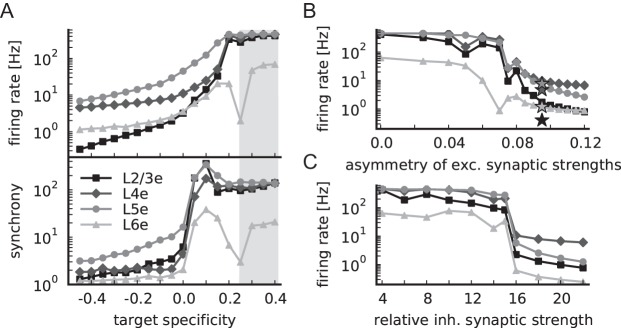
Relevance of target specificity for network stability. (A) Population firing rates (top panel) and synchrony (bottom panel), both in logarithmic representation, as a function of the target specificity of candidate projections L2/3e to L4, L2/3e to L6, L5e to L2/3, and L6e to L4, see Supplementary Table 3 for corresponding connection probabilities. A target specificity of zero reflects random connectivity; the gray-shaded area marks the range of target specificity of other interlayer connections (0.33 ± 0.08). (B) Population firing rates of the model with target specificity of candidate projections of +0.4 as a function of the asymmetry of excitatory to inhibitory and excitatory to excitatory synaptic strengths (defined as (wie − wee)/(wie + wee), with fixed mean excitatory synaptic strength). Stars indicate firing rates of the reference model with target specificity of candidate projections of −0.4. (C) As B, but as a function of the relative inhibitory synaptic strength. All markers as in Figure 8A.
The modification of target specificity not only changes the local microcircuit at the level of specific cell types but also the overall level of excitation in the network. Therefore, we simulate further control networks that globally correct for the change in the level of excitation: We induce an asymmetry of the excitatory synaptic strengths by increasing for all connections, not only for the i-specific candidates, the synaptic strength of excitatory to inhibitory connections and simultaneously reduce the synaptic strength of excitatory to excitatory connections. Figure 9B shows that a sufficiently large asymmetry of excitatory synaptic strengths counterbalances the overexcitation. However, the order of the excitatory activity levels of the cortical layers is partly inverted, that is, it is not consistent with the experimental activity data summarized in Table 6.
This stabilization procedure uses different excitatory synaptic strengths according to the target cell type and thereby introduces an additional parameter. We also investigate whether the network can alternatively be stabilized by changing an already existing parameter, the relative inhibitory synaptic strength. We find that only implausibly large values (g> 15) lead to a stable low-rate AI state (Fig. 9C) and that also in this case the order of firing rates is partly inverted.
In summary, the data-based layered network model that is parameterized equivalent to the balanced random network model requires the inclusion of i-specific feedback connections in order to exhibit AI spiking activity. The alternative stabilization of the network by global changes of parameters results in a distribution of layer-specific firing rates in conflict with experimental observations.
Propagation of Transient Thalamic Inputs
Confronted with a transient thalamic input, the layered network model responds with a stereotypical propagation of activity through the different layers. Figure 10A shows an exemplary spike raster of the model after a short-lasting increase of the thalamic firing rate. The cell-type specific activity pattern is consistent over 100 different network and input instantiations (Fig. 10B).
Figure 10.

Response to transient thalamic input. Thalamic firing rates increase step-like by 15 Hz for a duration of 10 ms; 0 ms corresponds to the onset of transient input, gray bars show the arrival of thalamic spikes at cortical neurons taking the mean delay (for simplicity the same as within the network, 1.5 ms) into account. (A) Cell-type specific spiking activity of the network with i-specific projections. Markers as in Figure 6A. (B) Corresponding cell-type specific population spike counts averaged over 100 instantiations of network and input (excitatory populations in black, inhibitory in gray). Spike counts are calculated with a bin width of 0.5 ms with the number of recorded neurons L3e: 500, L3i: 141, L4e: 529, L4i: 132, L5e: 117, L5i: 25, L6e: 347, L6i: 71 (numbers correspond to relative population sizes). (C) Spiking activity of a control network without i-specific projections (target specificity of candidate projections of +0.4) stabilized by an asymmetry of excitatory synaptic strengths of 0.095. (D) Corresponding cell-type specific population spike counts of excitatory populations averaged over 100 instantiations. Filled area shows the difference of the data in D and B. (E) Average percentage of cells in the excitatory populations that are activated by thalamic stimulation in relation to the ongoing activity (according to the data in B). (F) Dynamical gain, defined as the firing rate during the stimulus presentation divided by the spontaneous firing rate, of excitatory populations (according to the data in B).
Amplitude and Timing of Cell-Type Specific Responses
L2/3e, L4e, and L5e emit a comparable amount of additional spikes in response to the stimulus, while L6e shows a comparatively sparse response (Fig. 10B). In total, only a minority of all neurons in the network is activated by the thalamic stimulus (Fig. 10E). Only in L5e, a large fraction of all cells emits additional spikes in response to the stimulus. In relation to the ongoing activity, we find that the input layers (L4 and L6) exhibit a similar dynamical gain, which is much lower than the gain of the output layers L5 and particularly L2/3.
The response is initiated in the input layers and then propagates to L2/3 and L5 (Fig. 10A,B). The latency of activation (defined as the maximum of the excitatory spike count histogram) is shortest in L4 followed by L6 and L5, and finally L2/3. The early onset of activation of L5, not after but rather synchronously with L2/3, is in contrast to the expectation according to the classical notion of the feed-forward loop from L4 to L2/3 to L5 (Gilbert 1983), but in agreement with the experimental activity data (Sakata and Harris 2009, compare also Mitzdorf 1985). The difference in the latency of activation (defined as the time of the peak of the PSTH, compare also Sakata and Harris 2009) between the input layers and the output layers in our network is with around 2–3 ms below the experimentally observed latencies (5–10 ms according to Schroeder et al. (1998); Sakata and Harris (2009)). The feed-forward connection from L2/3 to L5 causes the prolonged response in L5 that is reflected in the second peak in the spike count. L6, being already slightly excited by the thalamic input, receives feed-forward input from L5 that triggers a sparse response during the ramp-up phase in L5. The activity is back to baseline in all layers before the last thalamic spikes arrive at cortex. Deactivation is ordered similar to activation, starting in L4, followed by L2/3 and L6, and finally L5.
Interplay of Excitation and Inhibition in the Propagation of Inputs
Not only the excitatory populations, but also the inhibitory populations show a distinct activation pattern (see Fig. 10A, gray dots, and B, gray lines). Initially, as the interneurons in any layer receive the same, albeit slightly weaker, feed-forward inputs, the inhibitory response resembles the excitatory response. However, the inhibitory populations show, in contrast to the respective excitatory populations, 2 pronounced activation peaks in L2/3, L4, and L6. As shown above, these layers receive i-specific feedback connections. Apparently, the cell-type specific connectivity structure results in a complex interplay of excitation and inhibition not explained by within-layer recurrent inhibition and thereby shapes the propagating response to a transient thalamic input. Specifically, we observe that the activation of L2/3 entails the increased activity of inhibitory interneurons in L4, thereby stopping the excitatory activity in this layer. A similar effect is observed in the next step of the feed-forward loop between L2/3 and L5. The activation of L2/3 prolongs the excitatory activity in L5 as stated above. In contrast, the early activation of L5 results in a sharpening of the response in L2/3 by the additional activation of L2/3 interneurons. The connection from L6e to L4i adds to the sharpening of the L4 response and the rather weak i-specific connection from L2/3 to L6 plays a role in preventing a stronger ramp-up of excitatory activity in L6.
Role of I-Specific Feedback Connections for the Propagation of Inputs
These observations suggest that the i-specific feedback connections control the duration and the amplitude of the response to thalamic inputs. To further elucidate their role for the propagation of input-related activity, we study the response of a network without i-specific feedback connections, but similar spontaneous activity. The small differences in the firing rates (compare Fig. 9B) are reflected in the initial response of the network to the thalamic input (first bumps in the spike count histograms in Fig. 11D), which exhibits a steeper increase in L2/3e and L4e and is weaker in L5e. After this initial phase, the response is drastically different and shows reverberating activation of the different layers lingering well beyond the offset of the input. The response is much stronger and shows oscillatory components by reciprocal activation of the different layers. The effect stays the same, albeit smaller, for a control network with the candidate projections having a target specificity value of +0.2, which is well below the range for nonspecific interlayer connections.
Figure 11.

Flow of activity following transient thalamic input. Black and gray ellipses represent excited and inhibited activity states, respectively. Dark gray dashed arrows indicate input and output of the local network. The black arrows represent the feed-forward loop projections L4 to L2/3 to L5 to L6. The gray arrows correspond to the activation of the candidate i-specific connections (L2/3e to L4 and to L6, L5e to L2/3, and L6e to L4).
Discussion
In this work, we employ full-scale spiking network modeling to relate the connectivity structure of the cortical microcircuit to its activity. To this end, we first provide an analysis of the currently used connectivity maps and integrate these into a map incorporating additional knowledge from functional connectivity studies. The integrated map yields, in a spiking network model, realistic cell-type specific spontaneous firing rates and captures the flow of activity through the different layers for stimulus-evoked activity. These findings depend on the specific target type selection of a subset of interlayer connections, which has largely been neglected by previous models.
Modeling Approach
The present work extends the balanced random network model (van Vreeswijk and Sompolinsky 1996, 1998; Amit and Brunel 1997; Brunel 2000) to multiple layers with realistic connection probabilities. Despite their reduced structure, the mono-layered models exhibit qualitatively consistent activity dynamics and the classical analysis of them has guided our research. Our neuron and synapse model as well as the random connectivity scheme do not differ qualitatively from the earlier work. Like in most network models with random connectivity, randomness here represents the simplest assumption (Amit 1989) and substitutes fine-scale structure addressed in other models (e.g. Lundqvist et al. 2010). Demanding global consistency of the random and the functionally motivated fine-scale structure will facilitate the reconciliation of the different approaches. The model size is selected sufficiently large to incorporate the majority of all local synapses. The network structure, one excitatory and one inhibitory population in each layer, represents the minimal laminar extension of the mono-layered models and also the minimal set of cell types typically distinguished in experiments. Data resolving the connectivity at a finer scale (e.g. Mercer et al. 2005; West et al. 2006) are combined to match the more coarse resolution of our model. Previous multilayered models partly use the same approach (e.g. Haeusler and Maass 2007) and partly more detailed cell-type classifications (e.g. Traub et al. 2005; Izhikevich and Edelman 2008). However, quantitative connectivity data are not yet widely and consistently available on a finer level of detail for neither anatomy nor physiology. The dynamical consequences of any further separation of cell types remain unclear. The model provides a building block for further modeling studies: Wagatsuma et al. (2011) apply the network model in the context of attentional modulation in the visual cortex and Lindén et al. (2011) employ the simulated spiking activity in combination with morphologically detailed single-neuron models to create a biologically realistic model of the local field potential.
Integrated Connectivity Map
The success of the dynamical analysis in the second part of the study relies on our finding that the 2 connectivity maps are consistent when one considers the differences in methodology. The compiled connectivity map accounts for these, but it nevertheless merges data not only from multiple laboratories, but also from different cortical areas and species. Although this choice is driven by the incompleteness of data for a specific area and species, we focus on 2 species, cat and rat. Primarily, the data originate from cat area 17 and rat primary visual and primary somatosensory areas. The density of neurons in our model is based on cat area 17 and the density of synapses is consistent with the cat data (Beaulieu and Colonnier 1985). The most crucial difference between our map and the original data-based maps is the target specific structure that removes the systematic biases introduced by the undersampling of inhibitory cells (electrophysiology) and the application of Peters' rule (anatomy).
The integrated connectivity map is consistent with the most prominent features of the cortical microcircuit: The recurrence of connections (Douglas et al. 1989; Douglas and Martin 1991) and the feed-forward loop from L4 to L2/3 to L5 to L6 to L4 (Gilbert 1983). The excitatory subcircuit is largely consistent with the recently published excitatory map of the C2 barrel column of the mouse (Lefort et al. 2009). In addition, the circuit exhibits a distinct feedback structure with projections targeting predominantly interneurons most notably from L2/3e to L4 and from L5e to L2/3. Thomson, Bannister, et al. (2002) and Thomson and Morris (2002) recognized the potential of selective feedback projections for stabilizing the activity and increasing the sensitivity for time-dependent signaling, but were unable to test this hypothesis. Here, we quantify the dynamical relevance of these i-specific projections and find that they are crucial for the stability and the reliability of spontaneous activity and evoked input propagation. Extending the idea of i-specific feedback, it is a conceivable, but untested, hypothesis that L6e cells target predominantly interneurons in L5, too.
The connectivity of L6 still poses several open questions (see Briggs 2010; Thomson 2010; for recent reviews). According to our estimate, L6 is the main recipient of external inputs (Table 3) primarily based, however, on indirect evidence of missing asymmetric synapses. In addition, some input pathways to this layer, for example, from L4 (Thomson 2010, see also Tarczy-Hornoch et al. 1999), are not sufficiently quantified to be incorporated in the integrated map. Likewise, outputs from L6 interneurons, for example, Martinotti cells projecting to superficial layers (Wang et al. 2004), are not included. We identify the projection from L6e to L4 as 1 of the 4 i-specific projections (Table 2) based on the EM study in the cat by McGuire et al. (1984), providing sparse and partial data. In their discussion, Ahmed et al. (1994) present an alternative interpretation of these data, proposing that many synapses originally assigned to inhibitory targets are potentially on excitatory cells. Still the authors acknowledge that the relative number of synapses targeting interneurons is very high in comparison with other excitatory projections. Staiger et al. (1996) report contrasting evidence in the rat so that further clarification is needed.
Model Parameterization
Today, only a subset of the model parameters is experimentally known. Here, we focus on cell-type specific structural parameters: The numbers of neurons, the numbers of external inputs, and the connection probabilities between neurons. Other parameters like neuronal parameters, synaptic strengths, and delays are selected independent of the cell type, based on the balanced random network model (Brunel 2000). The consistency of the activity in our model with the experimental data suggests that the (static) connectivity structure plays a dominant role in shaping the neuronal activity and that it is not required to model complex neuronal features such as morphology to reproduce the particular experimental findings discussed here.
An exception to the cell-type independent parameterization is the increased synaptic strength for the connection from L4e to L2/3e. Although this change affects the ongoing activity only marginally (Supplementary Fig. 7), it is important for a successful transmission of activity from L4 to L2/3 following thalamic stimulation. The modification is motivated by the large discrepancies of the L4i to L2/3 projection in the anatomical and physiological maps and the difference in the relative convergence of excitatory inputs from L2/3 and L4 to L2/3 pyramids between our model and Feldmeyer et al. (2006), see the caption to Supplementary Figure 7. To ultimately resolve this issue, it might be necessary to incorporate additional specificity (Yoshimura et al. 2005; Sarid et al. 2007; Fares and Stepanyants 2009) and, despite a plethora of studies on the L4 to L2/3 connections, potentially additional experiments especially regarding the inhibitory projection.
Spontaneous Cell-Type Specific Activity
The application of the integrated connectivity map and the parameterization according to the balanced random network models results in AI activity without specific tuning, indicating that the properties of the mono-layered model generalize to the multilayered network. This activity state is stable over a wide range of parameters regarding, for example, external inputs, synaptic strengths, and delays.
The model predicts cell-type specific firing rates in agreement with data from awake animals (Table 6). In particular, the connectivity map captures the low excitatory firing rates in L2/3 and L6 quantitatively, although mono-layered models hardly show stable activity at these low levels of activity (Sussillo et al. 2007). Due to the parameterization, the increase of inhibitory firing rates in all layers compared with the respective excitatory rates can be attributed to the network structure. L4e and L5e show the appropriate ranking but slightly higher firing rates than observed experimentally. We expect that the inclusion of further cell-type specificity would yield a closer match of simulations and experimental observations. For example in L5, a fine-scale structure has been observed between L5 pyramids and Martinotti cells, which efficiently counteracts transient increases in L5e firing rates (Silberberg and Markram 2007; Berger et al. 2010) and involves short-term synaptic facilitation.
The fact that other contemporary models have difficulties in matching the observed cell-type specific activity potentially relates to the employed connectivity maps: Only our integrated map features the i-specific connections in combination with the detailed mapping from anatomy and physiology. Rasch et al. (2011), using the physiological data of Thomson, West, et al. (2002), observe that it is necessary to increase the synaptic strength of excitatory to inhibitory connections in order to produce a realistic firing regime. Although their work takes a more detailed approach to model neuronal dynamics and synaptic interactions, this specific finding may relate to the properties of the applied connectivity map: Our investigation of target specificity reveals that the straightforward application of the physiological data likely introduces a bias to purely excitatory to excitatory interlayer connections (Fig. 4). Furthermore, in our integrated map, the particular ordering by firing rate depends on the inclusion of i-specific feedback connections. Increasing the excitatory to inhibitory synaptic strength globally compensates for missing i-specific connections, but destroys the consistency of the simulated and observed firing rates (Fig. 9B).
Flow of Activity
Confronted with transient thalamic input, the model exhibits a particular propagation of activity from the input layers to the output layers (compare Miller 1996). The propagation pattern (Fig. 11) is shaped by the interaction of excitation and inhibition between the different layers and promotes a temporal neural code (Thomson and Morris 2002): Excitatory feed-forward projections determine the spread of excitation, while i-specific feedback shapes the temporal structure of the response. The propagation pattern in our simulations matches those observed in in vivo experiments of awake rats (Sakata and Harris 2009), although a detailed comparison is difficult as the thalamic activation in the experiments is not known. The difference in latencies of activation between input and output layers exhibits slightly faster timescales in our model than in experiments (Schroeder et al. 1998; Sakata and Harris 2009). This discrepancy may originate in different properties of the thalamic input patterns or in longer synaptic delays for interlayer connections than used in our model. Additional fine-scale structure, for example, inhibitory subtypes or functionally distinct neuronal populations (e.g. Beierlein et al. 2003; Yoshimura and Callaway 2005), would also contribute to more complex activations with a correspondingly increased average latency of activation.
The interactions between L4 and L2/3 and between L2/3 and L5 can be understood as a notification or handshake principle: The sender of information, for example, L4, is notified by the receiver, L2/3, that the information is being processed. This takes place in the local microcircuit by the i-specic projection from L2/3 to L4 interneurons, which can use the additional excitation to reduce (or reset) the activity of L4 excitatory cells. This circuit design contributes to shaping the flow of activity through the local network after thalamic stimulation. The same notification principle may hold also for other projections within and outside of the local microcircuit. The notification principle may be considered in addition to other ideas on cortical operation like the “just-enough and just-in-time” principle (Douglas and Martin 2007a) as it is concerned neither with the forward propagation of information nor the actual calculation, but with the preparation for the next operation. A prediction of this hypothesis is, for example, the response of L4 excitatory cells in the context of attentional modulation, which exhibits inverse tendencies compared with L2/3 and L5 (Wagatsuma et al. 2011).
Relation of Structure and Activity
The cell-type specific input structure of the integrated map (Fig. 12) sheds light on the mechanisms underlying the observed activity features. For example, the low firing rates of L2/3e and L6e neurons in our model have different structural origins: L2/3e effectively integrates, next to the excitatory inputs from L2/3e and L4e, inhibitory inputs from all layers. In contrast, L6e interacts largely with the recurrent within-L6 network; other inputs predominantly pass through L5e and rather modulate L6e activity. L4e is also dominated by within-layer connectivity, and the i-specific inputs from L2/3 and L6 modulate its activity and temporally structure the response to transient stimuli. L5 consists of relatively few neurons and correspondingly forms rather few recurrent within-layer inputs. Furthermore, L5e integrates the highest number of first-order inputs and does not receive i-specific projections. As a result, L5e reacts with a wide range of firing rates to changes in the external input, particularly in comparison with the other layers. This, together with the control that L5 exerts on L2/3 by the i-specific feedback, puts it in a special position to integrate and amplify information. Inhibitory cells receive predominantly excitatory interlayer inputs (Supplementary Fig. 5) and therefore exhibit elevated firing rates.
Figure 12.
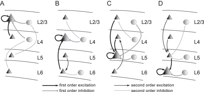
Input structure for the excitatory cell types L2/3e (A), L4e (B), L5e (C), and L6e (D) (large triangles). The illustrations show the strongest pathways, that is, only connection probabilities >0.04 are considered, of direct (first order, thick arrows) and indirect (second order, thin arrows) excitation (black) and inhibition (gray) of a given population (see Supplementary Material for further details). Triangles represent excitatory and circles inhibitory populations.
Outlook
Our microcircuit model successfully reproduces prominent features of cortical activity based on minimal constituents, leaky integrate-and-fire model neurons interacting by static synapses, lacking features such as short-term plasticity, adaptation, or complex morphologies, which affect the dynamics of the network. This suggests that these neuronal and synaptic features are relevant to more complex tasks performed by the cortical microcircuit (see, e.g., Fujisawa et al. 2008; Gutnisky and Dragoi 2008; Mongillo et al. 2008), but not to support the spontaneous activity or rapid propagation of transient inputs. To elucidate the role of these features, functional studies based on more complex inputs and potentially incorporating functional fine-scale connectivity structure (e.g. Sporns and Kötter 2004; Yoshimura et al. 2005) and the lateral intrinsic network (Rockland and Lund 1982; Douglas and Martin 2004) have to be conducted. In this context, also more complex distributions of synaptic strengths (e.g. long-tail distributions, Teramae et al. 2012) may become relevant.
Complementing the sophistication of network structures and the constituent's dynamics, further theoretical work is required to fully understand the properties of the microcircuit model (e.g. Tetzlaff et al. 2012). Reduced models like an 8-dimensional mean-field description (see Deco et al. 2011, for a recent overview) will enable a more comprehensive investigation of the model's parameter space.
Ultimately, it is indispensable to bridge the scales between the microcircuit and the macroscopic connectivity (Felleman and Van Essen 1991; Reid et al. 2009) to understand the interactions of the local network with other parts of the brain. We suppose that brain-scale models will allow for self-consistent descriptions of neuronal activity dynamics: Networks of networks incorporating subcortical feedback loops and multiple brain areas (Sporns et al. 2005) will provide realistic inputs to the local cortical network and simultaneously enable a consistency check of microscopic and macroscopic activity patterns (Fox et al. 2005; Deco et al. 2009).
Conclusion
The connectivity structure of the local cortical network shapes the cell-type specific activity and defines functional roles of the different layers. Any fine-scale connectivity structure (e.g. Song et al. 2005; Yoshimura et al. 2005; Kampa et al. 2006) faces the constraints imposed by the connectivity implemented in this model. The presented framework can be continuously refined as new data become available and extends the available mathematical methods to infer synaptic connectivity from neuronal morphology. Based on the currently available data, it reproduces prominent activity features, suggesting that these arise predominantly from network structure, not single cell properties. The results predict distinct activity patterns of interneurons and highlight the need to uncover the target specificity of projections in future experiments.
Supplementary Material
Supplementary material can be found at: http://www.cercor.oxfordjournals.org/
Funding
This work was supported by the Helmholtz Alliance on Systems Biology; European Union (FACETS, grant 15879 and BrainScaleS, grant 269921); Deutsch-Israelische Projektkooperation (DIP, grant F1.2); Bundesministerium für Bildung und Forschung, Germany (BMBF, grant 01GQ0420 to BCCN Freiburg), and the Next-Generation Supercomputer Project of the Ministry of education, culture, sports, science and technology (MEXT), Japan. Funding to pay the Open Access publication charges for this article was provided by Research Center Juelich a member of the Helmholtz Association.
Supplementary Material
Notes
We are grateful to Kathleen S. Rockland and Dirk Feldmeyer for fruitful discussions about the structure of the local cortical network and to our colleagues in the NEST Initiative for continued support. Conflict of Interest: None declared.
References
- Ahmed B, Anderson J, Douglas R, Martin K, Nelson J. Polyneuronal innervation of spiny stellate neurons in cat visual cortex. J Compar Neurol. 1994;341:39–49. doi: 10.1002/cne.903410105. doi:10.1002/cne.903410105. [DOI] [PubMed] [Google Scholar]
- Ali AB, Bannister AP, Thomson AM. Robust correlations between action potential duration and the properties of synaptic connections in layer4 interneurones in neocortical slices from juvenile rats and adult rat and cat. J Physiol (Lond) 2007;580:149–169. doi: 10.1113/jphysiol.2006.124214. doi:10.1113/jphysiol.2006.124214. [DOI] [PMC free article] [PubMed] [Google Scholar]
- Amit DJ. Modeling brain function. Cambridge, NY: Cambridge University Press; 1989. [Google Scholar]
- Amit DJ, Brunel N. Model of global spontaneous activity and local structured activity during delay periods in the cerebral cortex. Cereb Cortex. 1997;7:237–252. doi: 10.1093/cercor/7.3.237. doi:10.1093/cercor/7.3.237. [DOI] [PubMed] [Google Scholar]
- Bannister AP, Thomson AM. Dynamic properties of excitatory synaptic connections involving layer 4 pyramidal cells in adult rat and cat neocortex. Cereb Cortex. 2007;17:2190–2203. doi: 10.1093/cercor/bhl126. doi:10.1093/cercor/bhl126. [DOI] [PubMed] [Google Scholar]
- Beaulieu C, Colonnier M. A laminar analysis of the number of round-asymmetrical and flat-symmetrical synapses on spines, dendritic trunks, and cell bodies in area 17 of the cat. J Compar Neurol. 1985;231:180–189. doi: 10.1002/cne.902310206. doi:10.1002/cne.902310206. [DOI] [PubMed] [Google Scholar]
- Beaulieu C, Colonnier M. The number of neurons in the different laminae of the binocular and monocular regions of area 17 in the cat. J Compar Neurol. 1983;217:337–344. doi: 10.1002/cne.902170308. doi:10.1002/cne.902170308. [DOI] [PubMed] [Google Scholar]
- Beierlein M, Connors BW. Short-term dynamics of thalamocortical and intracortical synapses onto layer 6 neurons in neocortex. J Neurophysiol. 2002;88:1924–1932. doi: 10.1152/jn.2002.88.4.1924. [DOI] [PubMed] [Google Scholar]
- Beierlein M, Gibson JR, Connors BW. Two dynamically distinct inhibitory networks in layer 4 of the neocortex. J Neurophysiol. 2003;90:2987–3000. doi: 10.1152/jn.00283.2003. doi:10.1152/jn.00283.2003. [DOI] [PubMed] [Google Scholar]
- Berger TK, Silberberg G, Perin R, Markram H. Brief bursts self-inhibit and correlate the pyramidal network. PLoS Biol. 2010;8:e1000473. doi: 10.1371/journal.pbio.1000473. doi:10.1371/journal.pbio.1000473. [DOI] [PMC free article] [PubMed] [Google Scholar]
- Binzegger T, Douglas RJ, Martin KAC. A quantitative map of the circuit of cat primary visual cortex. J Neurosci. 2004;39:8441–8453. doi: 10.1523/JNEUROSCI.1400-04.2004. doi:10.1523/JNEUROSCI.1400-04.2004. [DOI] [PMC free article] [PubMed] [Google Scholar]
- Binzegger T, Douglas RJ, Martin KAC. Stereotypical bouton clustering of individual neurons in cat primary visual cortex. J Neurosci. 2007;27:12242–12254. doi: 10.1523/JNEUROSCI.3753-07.2007. doi:10.1523/JNEUROSCI.3753-07.2007. [DOI] [PMC free article] [PubMed] [Google Scholar]
- Binzegger T, Douglas RJ, Martin KAC. Topology and dynamics of the canonical circuit of cat V1. Neural Netw. 2009;22:1071–1078. doi: 10.1016/j.neunet.2009.07.011. doi:10.1016/j.neunet.2009.07.011. [DOI] [PubMed] [Google Scholar]
- Braitenberg V, Schüz A. Cortex: statistics and geometry of neuronal connectivity. 2nd ed. Berlin: Springer-Verlag; 1998. [Google Scholar]
- Brémaud A, West DC, Thomson AM. Binomial parameters differ across neocortical layers and with different classes of connections in adult rat and cat neocortex. Proc Nat Acad Sci USA. 2007;104:14134–14139. doi: 10.1073/pnas.0705661104. doi:10.1073/pnas.0705661104. [DOI] [PMC free article] [PubMed] [Google Scholar]
- Briggs F. Organizing principles of cortical layer 6. Front Neural Circuits. 2010;4:3. doi: 10.3389/neuro.04.003.2010. [DOI] [PMC free article] [PubMed] [Google Scholar]
- Brunel N. Dynamics of sparsely connected networks of excitatory and inhibitory spiking neurons. J Comput Neurosci. 2000;8:183–208. doi: 10.1023/a:1008925309027. doi:10.1023/A:1008925309027. [DOI] [PubMed] [Google Scholar]
- Buzas P, Kovacs K, Ferecsko AS, Budd JML, Eysel UT, Kisvarday ZF. Model-based analysis of excitatory lateral connections in the visual cortex. J Compar Neurol. 2006;499:861–881. doi: 10.1002/cne.21134. doi:10.1002/cne.21134. [DOI] [PubMed] [Google Scholar]
- Crochet S, Petersen CCH. Correlating whisker behavior with membrane potential in barrel cortex of awake mice. Nat Neurosci. 2006;9:608–610. doi: 10.1038/nn1690. doi:10.1038/nn1690. [DOI] [PubMed] [Google Scholar]
- Dantzker JL, Callaway EM. Laminar sources of synaptic input to cortical inhibitory interneurons and pyramidal neurons. Nat Neurosci. 2000;3:701–707. doi: 10.1038/76656. doi:10.1038/76656. [DOI] [PubMed] [Google Scholar]
- Deco G, Jirsa VK, McIntosh AR. Emerging concepts for the dynamical organization of resting-state activity in the brain. Nat Rev Neurosci. 2011;12:43–56. doi: 10.1038/nrn2961. doi:10.1038/nrn2961. [DOI] [PubMed] [Google Scholar]
- Deco G, Jirsa V, McIntosh AR, Sporns O, Kötter R. Key role of coupling, delay, and noise in resting brain fluctuations. Proc Natl Acad Sci U S A. 2009;106:10302–10307. doi: 10.1073/pnas.0901831106. doi:10.1073/pnas.0901831106. [DOI] [PMC free article] [PubMed] [Google Scholar]
- de Kock CPJ, Sakmann B. Spiking in primary somatosensory cortex during natural whisking in awake head-restrained rats is cell-type specific. Proc Natl Acad Sci U S A. 2009;106:16446–16450. doi: 10.1073/pnas.0904143106. doi:10.1073/pnas.0904143106. [DOI] [PMC free article] [PubMed] [Google Scholar]
- Djurfeldt M, Hjorth J, Eppler JM, Dudani N, Helias M, Potjans TC, Bhalla US, Diesmann M, Hellgren Kotaleski J, Ekeberg Ö. Run-time interoperability between neuronal network simulators based on the MUSIC framework. Neuroinformatics. 2010;8:43–60. doi: 10.1007/s12021-010-9064-z. doi:10.1007/s12021-010-9064-z. [DOI] [PMC free article] [PubMed] [Google Scholar]
- Djurfeldt M, Lundqvist M, Johansson C, Rehn M, Ekeberg O, Lansner A. Brain-scale simulation of the neocortex on the IBM Blue Gene/L supercomputer. IBM J Res Develop. 2008;52:31–41. doi:10.1147/rd.521.0031. [Google Scholar]
- Douglas RJ, Martin KAC. The butterfly and the loom. Brain Res Bull. 2007b;55:314–328. doi: 10.1016/j.brainresrev.2007.04.011. [DOI] [PubMed] [Google Scholar]
- Douglas RJ, Martin KAC. A functional microcircuit for cat visual cortex. J Physiol (Lond) 1991;440:735–769. doi: 10.1113/jphysiol.1991.sp018733. [DOI] [PMC free article] [PubMed] [Google Scholar]
- Douglas RJ, Martin KAC. Mapping the matrix: the ways to neocortex. Neuron. 2007a;56:226–238. doi: 10.1016/j.neuron.2007.10.017. doi:10.1016/j.neuron.2007.10.017. [DOI] [PubMed] [Google Scholar]
- Douglas RJ, Martin KAC. Neuronal circuits of the neocortex. Annu Rev Neurosci. 2004;27:419–451. doi: 10.1146/annurev.neuro.27.070203.144152. doi:10.1146/annurev.neuro.27.070203.144152. [DOI] [PubMed] [Google Scholar]
- Douglas RJ, Martin KAC, Whitteridge D. A canonical microcircuit for neocortex. Neural Comput. 1989;1:480–488. doi:10.1162/neco.1989.1.4.480. [Google Scholar]
- Eppler JM, Helias M, Muller E, Diesmann M, Gewaltig M. PyNEST: a convenient interface to the NEST simulator. Front Neuroinform. 2009;2:12. doi: 10.3389/neuro.11.012.2008. [DOI] [PMC free article] [PubMed] [Google Scholar]
- Fares T, Stepanyants A. Cooperative synapse formation in the neocortex. Proc Natl Acad Sci U S A. 2009;106:16463–16468. doi: 10.1073/pnas.0813265106. doi:10.1073/pnas.0813265106. [DOI] [PMC free article] [PubMed] [Google Scholar]
- Feldmeyer D, Lübke J, Sakmann B. Efficacy and connectivity of intracolumnar pairs of layer 2/3 pyramidal cells in the barrel cortex of juvenile rats. J Physiol (Lond) 2006;575:583–602. doi: 10.1113/jphysiol.2006.105106. doi:10.1113/jphysiol.2006.105106. [DOI] [PMC free article] [PubMed] [Google Scholar]
- Feldmeyer D, Lübke J, Silver RA, Sakmann B. Synaptic connections between layer 4 spiny neurone-layer 2/3 pyramidal cell pairs in juvenile rat barrel cortex: physiology and anatomy of interlaminar signalling within a cortical column. J Physiol (Lond) 2002;538:803–822. doi: 10.1113/jphysiol.2001.012959. doi:10.1113/jphysiol.2001.012959. [DOI] [PMC free article] [PubMed] [Google Scholar]
- Feldmeyer D, Roth A, Sakmann B. Monosynaptic connections between pairs of spiny stellate cells in layer 4 and pyramidal cells in layer 5a indicate that lemniscal and paralemniscal afferent pathways converge in the infragranular somatosensory cortex. J Neurosci. 2005;25:3423–3431. doi: 10.1523/JNEUROSCI.5227-04.2005. doi:10.1523/JNEUROSCI.5227-04.2005. [DOI] [PMC free article] [PubMed] [Google Scholar]
- Felleman DJ, Van Essen DC. Distributed hierarchical processing in the primate cerebral cortex. Cereb Cortex. 1991;1:1–47. doi: 10.1093/cercor/1.1.1-a. doi:10.1093/cercor/1.1.1-a. [DOI] [PubMed] [Google Scholar]
- Fetz E, Toyama K, Smith W. Synaptic interactions between cortical neurons. In: Peters A, editor. Cerebral cortex. Vol. 9. New York, London: Plenum Press; 1991. pp. 1–47. Chapter 1. [Google Scholar]
- Fox MD, Snyder AZ, Vincent JL, Corbetta M, Van Essen DC, Raichle ME. The human brain is intrinsically organized into dynamic, anticorrelated functional networks. Proc Natl Acad Sci U S A. 2005;102:9673–9678. doi: 10.1073/pnas.0504136102. doi:10.1073/pnas.0504136102. [DOI] [PMC free article] [PubMed] [Google Scholar]
- Fujisawa S, Amarasingham A, Harrison MT, Buzsáki G. Behavior-dependent short-term assembly dynamics in the medial prefrontal cortex. Nat Neurosci. 2008;11:823–833. doi: 10.1038/nn.2134. doi:10.1038/nn.2134. [DOI] [PMC free article] [PubMed] [Google Scholar]
- Gabbott PL, Somogyi P. Quantitative distribution of GABA-immunoreactive neurons in the visual cortex (area 17) of the cat. Exp Brain Res. 1986;61:323–331. doi: 10.1007/BF00239522. [DOI] [PubMed] [Google Scholar]
- Gewaltig M-O, Diesmann M. NEST (NEural Simulation Tool) Scholarpedia. 2007;2:1430. doi:10.4249/scholarpedia.1430. [Google Scholar]
- Gilbert CD. Laminar differences in receptive field properties of cells in cat primary visual cortex. J Physiol (Lond) 1977;268:391–421. doi: 10.1113/jphysiol.1977.sp011863. [DOI] [PMC free article] [PubMed] [Google Scholar]
- Gilbert CD. Microcircuitry of the visual cortex. Annu Rev Neurosci. 1983;6:217–247. doi: 10.1146/annurev.ne.06.030183.001245. doi:10.1146/annurev.ne.06.030183.001245. [DOI] [PubMed] [Google Scholar]
- Gilbert CD, Wiesel TN. Clustered intrinsic connections in cat visual cortex. J Neurosci. 1983;5:1116–33. doi: 10.1523/JNEUROSCI.03-05-01116.1983. [DOI] [PMC free article] [PubMed] [Google Scholar]
- Golomb D. Neuronal synchrony measures. Scholarpedia. 2007;2:1347. doi:10.4249/scholarpedia.1347. [Google Scholar]
- Gonchar Y, Burkhalter A. Distinct GABAergic targets of feedforward and feedback connections between lower and higher areas of rat visual cortex. J Neurosci. 2003;23:10904–10912. doi: 10.1523/JNEUROSCI.23-34-10904.2003. [DOI] [PMC free article] [PubMed] [Google Scholar]
- Greenberg DS, Houweling AR, Kerr JND. Population imaging of ongoing neuronal activity in the visual cortex of awake rats. Nat Neurosci. 2008;11:749–751. doi: 10.1038/nn.2140. doi:10.1038/nn.2140. [DOI] [PubMed] [Google Scholar]
- Gutnisky DA, Dragoi V. Adaptive coding of visual information in neural populations. Nature. 2008;452:220–224. doi: 10.1038/nature06563. doi:10.1038/nature06563. [DOI] [PubMed] [Google Scholar]
- Haeusler S, Maass W. A statistical analysis of information-processing properties of lamina-specific cortical microcircuit models. Cereb Cortex. 2007;17:149–162. doi: 10.1093/cercor/bhj132. doi:10.1093/cercor/bhj132. [DOI] [PubMed] [Google Scholar]
- Haeusler S, Schuch K, Maass W. Motif distribution, dynamical properties, and computational performance of two data-based cortical microcircuit templates. J Physiol (Paris) 2009;103:73–87. doi: 10.1016/j.jphysparis.2009.05.006. doi:10.1016/j.jphysparis.2009.05.006. [DOI] [PubMed] [Google Scholar]
- Heimel JA, Van Hooser SD, Nelson SB. Laminar organization of response properties in primary visual cortex of the gray squirrel (sciurus carolinensis) J Neurophysiol. 2005;94:3538–3554. doi: 10.1152/jn.00106.2005. doi:10.1152/jn.00106.2005. [DOI] [PubMed] [Google Scholar]
- Heinzle J, Hepp K, Martin KAC. A microcircuit model of the frontal eye fields. J Neurosci. 2007;27:9341–9353. doi: 10.1523/JNEUROSCI.0974-07.2007. doi:10.1523/JNEUROSCI.0974-07.2007. [DOI] [PMC free article] [PubMed] [Google Scholar]
- Hellwig B. A quantitative analysis of the local connectivity between pyramidal neurons in layers 2/3 of the rat visual cortex. Biol Cybern. 2000;2:111–121. doi: 10.1007/PL00007964. doi:10.1007/PL00007964. [DOI] [PubMed] [Google Scholar]
- Hill S, Tononi G. Modeling sleep and wakefulness in the thalamocortical system. J Neurophysiol. 2005;93:1671–1698. doi: 10.1152/jn.00915.2004. doi:10.1152/jn.00915.2004. [DOI] [PubMed] [Google Scholar]
- Holmgren C, Harkany T, Svennenfors B, Zilberter Y. Pyramidal cell communication within local networks in layer 2/3 of rat neocortex. J Physiol (Lond) 2003;1:139–153. doi: 10.1113/jphysiol.2003.044784. doi:10.1113/jphysiol.2003.044784. [DOI] [PMC free article] [PubMed] [Google Scholar]
- Izhikevich EM. Polychronization: computation with spikes. Neural Comput. 2006;18:245–282. doi: 10.1162/089976606775093882. doi:10.1162/089976606775093882. [DOI] [PubMed] [Google Scholar]
- Izhikevich EM, Edelman GM. Large-scale model of mammalian thalamocortical systems. Proc Natl Acad Sci U S A. 2008;105:3593–3598. doi: 10.1073/pnas.0712231105. doi:10.1073/pnas.0712231105. [DOI] [PMC free article] [PubMed] [Google Scholar]
- Izhikevich EM, Gally JA, Edelman GM. Spike-timing dynamics of neuronal groups. Cereb Cortex. 2004;14:933–944. doi: 10.1093/cercor/bhh053. doi:10.1093/cercor/bhh053. [DOI] [PubMed] [Google Scholar]
- Johnson RR, Burkhalter A. Microcircuitry of forward and feedback connections within rat visual cortex. J Compar Neurol. 1996;368:383–398. doi: 10.1002/(SICI)1096-9861(19960506)368:3<383::AID-CNE5>3.0.CO;2-1. doi:10.1002/(SICI)1096-9861(19960506)368:3<383::AID-CNE5>3.0.CO;2-1. [DOI] [PubMed] [Google Scholar]
- Kampa BM, Letzkus JJ, Stuart GJ. Cortical feed-forward networks for binding different streams of sensory information. Nat Neurosci. 2006;9:1472–1473. doi: 10.1038/nn1798. doi:10.1038/nn1798. [DOI] [PubMed] [Google Scholar]
- Kapfer C, Glickfeld L, Atallah B, Scanziani M. Supralinear increase of recurrent inhibition during sparse activity in the somatosensory cortex. Nat Neurosci. 2007;10:743–753. doi: 10.1038/nn1909. doi:10.1038/nn1909. [DOI] [PMC free article] [PubMed] [Google Scholar]
- Kriener B, Tetzlaff T, Aertsen A, Diesmann M, Rotter S. Correlations and population dynamics in cortical networks. Neural Comput. 2008;20:2185–2226. doi: 10.1162/neco.2008.02-07-474. doi:10.1162/neco.2008.02-07-474. [DOI] [PubMed] [Google Scholar]
- Kumar A, Schrader S, Aertsen A, Rotter S. The high-conductance state of cortical networks. Neural Comput. 2008;20:1–43. doi: 10.1162/neco.2008.20.1.1. doi:10.1162/neco.2008.20.1.1. [DOI] [PubMed] [Google Scholar]
- Le Be J-V, Markram H. Spontaneous and evoked synaptic rewiring in the neonatal neocortex. Proc Natl Acad Sci USA. 2006;103:13214–13219. doi: 10.1073/pnas.0604691103. doi:10.1073/pnas.0604691103. [DOI] [PMC free article] [PubMed] [Google Scholar]
- Lee A, Manns I, Sakmann B, Brecht M. Whole-cell recordings in freely moving rats. Neuron. 2006;51:399–407. doi: 10.1016/j.neuron.2006.07.004. doi:10.1016/j.neuron.2006.07.004. [DOI] [PubMed] [Google Scholar]
- Lefort S, Tomm C, Sarria J-CF, Petersen CCH. The excitatory neuronal network of the C2 barrel column in mouse primary somatosensory cortex. Neuron. 2009;61:301–316. doi: 10.1016/j.neuron.2008.12.020. doi:10.1016/j.neuron.2008.12.020. [DOI] [PubMed] [Google Scholar]
- Lindén H, Tetzlaff T, Potjans TC, Pettersen KH, Grün S, Diesmann M, Einevoll GT. Modeling the spatial reach of the LFP. Neuron. 2011;72:859–872. doi: 10.1016/j.neuron.2011.11.006. doi:10.1016/j.neuron.2011.11.006. [DOI] [PubMed] [Google Scholar]
- Lundqvist M, Compte A, Lansner A. Bistable, irregular firing and population oscillations in a modular attractor memory network. PLoS Comput Biol. 2010;6:e1000803. doi: 10.1371/journal.pcbi.1000803. doi:10.1371/journal.pcbi.1000803. [DOI] [PMC free article] [PubMed] [Google Scholar]
- Lundqvist M, Rehn M, Djurfeldt M, Lansner A. Attractor dynamics in a modular network model of neocortex. Network. 2006;17:253–276. doi: 10.1080/09548980600774619. doi:10.1080/09548980600774619. [DOI] [PubMed] [Google Scholar]
- Maffei A, Nelson SB, Turrigiano GG. Selective reconfiguration of layer 4 visual circuitry by visual deprivation. Nat Neurosci. 2004;7:1353–1359. doi: 10.1038/nn1351. doi:10.1038/nn1351. [DOI] [PubMed] [Google Scholar]
- Markram H, Lübke J, Frotscher M, Roth A, Sakmann B. Physiology and anatomy of synaptic connections between thick tufted pyramidal neurons in the developing rat neocortex. J Physiol (Lond) 1997;500:409–440. doi: 10.1113/jphysiol.1997.sp022031. [DOI] [PMC free article] [PubMed] [Google Scholar]
- Martin KAC, Whitteridge D. Form, function, and intracortical projections of spiny neurons in the striate visual cortex of the cat. J Physiol (Lond) 1984;353:463–504. doi: 10.1113/jphysiol.1984.sp015347. [DOI] [PMC free article] [PubMed] [Google Scholar]
- Mason A, Nicoll A, Stratford K. Synaptic transmission between individual pyramidal neurons of the rat visual cortex in vitro. J Neurosci. 1991;11:72–84. doi: 10.1523/JNEUROSCI.11-01-00072.1991. [DOI] [PMC free article] [PubMed] [Google Scholar]
- McGuire BA, Hornung J-P, Gilbert CD, Wiesel TN. Patterns of synaptic input to layer 4 of cat striate cortex. J Neurosci. 1984;4:3021–3033. doi: 10.1523/JNEUROSCI.04-12-03021.1984. [DOI] [PMC free article] [PubMed] [Google Scholar]
- Mercer A, West DC, Morris OT, Kirchhecker S, Kerkhoff JE, Thomson AM. Excitatory connections made by presynaptic cortico-cortical pyramidal cells in layer 6 of the neocortex. Cereb Cortex. 2005;15:1485–1496. doi: 10.1093/cercor/bhi027. doi:10.1093/cercor/bhi027. [DOI] [PubMed] [Google Scholar]
- Miller R. Neural assemblies and laminar interactions in the cerebral cortex. Biol Cybern. 1996;75:253–261. doi: 10.1007/s004220050292. doi:10.1007/s004220050292. [DOI] [PubMed] [Google Scholar]
- Mitzdorf U. Current source-density method and application in cat cerebral cortex: investigation of evoked potentials and EEG phenomena. Physiol Rev. 1985;65:37–100. doi: 10.1152/physrev.1985.65.1.37. [DOI] [PubMed] [Google Scholar]
- Mongillo G, Barak O, Tsodyks M. Synaptic theory of working memory. Science. 2008;319:1543–1546. doi: 10.1126/science.1150769. doi:10.1126/science.1150769. [DOI] [PubMed] [Google Scholar]
- Morrison A, Aertsen A, Diesmann M. Spike-timing dependent plasticity in balanced random networks. Neural Comput. 2007;19:1437–1467. doi: 10.1162/neco.2007.19.6.1437. doi:10.1162/neco.2007.19.6.1437. [DOI] [PubMed] [Google Scholar]
- Morrison A, Mehring C, Geisel T, Aertsen A, Diesmann M. Advancing the boundaries of high connectivity network simulation with distributed computing. Neural Comput. 2005;17:1776–1801. doi: 10.1162/0899766054026648. doi:10.1162/0899766054026648. [DOI] [PubMed] [Google Scholar]
- Nordlie E, Gewaltig M-O, Plesser HE. Towards reproducible descriptions of neuronal network models. PLoS Comput Biol. 2009;5:e1000456. doi: 10.1371/journal.pcbi.1000456. doi:10.1371/journal.pcbi.1000456. [DOI] [PMC free article] [PubMed] [Google Scholar]
- Peters A, Payne BR. Numerical relationships between geniculocortical afferents and pyramidal cell modules in cat primary visual cortex. Cereb Cortex. 1993;3:69–78. doi: 10.1093/cercor/3.1.69. doi:10.1093/cercor/3.1.69. [DOI] [PubMed] [Google Scholar]
- Poulet J, Petersen C. Internal brain state regulates membrane potential synchrony in barrel cortex of behaving mice. Nature. 2008;454:881–885. doi: 10.1038/nature07150. doi:10.1038/nature07150. [DOI] [PubMed] [Google Scholar]
- Rasch MJ, Schuch K, Logothetis NK, Maass W. Statistical comparison of spike responses to natural stimuli in monkey area V1 with simulated responses of a detailed laminar network model for a patch of V1. J Neurophysiol. 2011;105:757–778. doi: 10.1152/jn.00845.2009. doi:10.1152/jn.00845.2009. [DOI] [PMC free article] [PubMed] [Google Scholar]
- Reid AT, Krumnack A, Wanke E, Kötter R. Optimization of cortical hierarchies with continuous scales and ranges. Neuroimage. 2009;47:611–617. doi: 10.1016/j.neuroimage.2009.04.061. doi:10.1016/j.neuroimage.2009.04.061. [DOI] [PubMed] [Google Scholar]
- Ren M, Yoshimura Y, Takada N, Horibe S, Komatsu Y. Specialized inhibitory synaptic actions between nearby neocortical pyramidal neurons. Science. 2007;316:758–761. doi: 10.1126/science.1135468. doi:10.1126/science.1135468. [DOI] [PubMed] [Google Scholar]
- Rockland KS, Lund JS. Widespread periodic intrinsic connections in the tree shrew visual cortex. Science. 1982;215:1532–1534. doi: 10.1126/science.7063863. doi:10.1126/science.7063863. [DOI] [PubMed] [Google Scholar]
- Sakata S, Harris KD. Laminar structure of spontaneous and sensory-evoked population activity in auditory cortex. Neuron. 2009;64:404–418. doi: 10.1016/j.neuron.2009.09.020. doi:10.1016/j.neuron.2009.09.020. [DOI] [PMC free article] [PubMed] [Google Scholar]
- Sarid L, Bruno R, Sakmann B, Segev I, Feldmeyer D. Modeling a layer 4-to-layer 2/3 module of a single column in rat neocortex: interweaving in vitro and in vivo experimental observations. Proc Natl Acad Sci U S A. 2007;104:16353–16358. doi: 10.1073/pnas.0707853104. doi:10.1073/pnas.0707853104. [DOI] [PMC free article] [PubMed] [Google Scholar]
- Schroeder CE, Mehta AD, Givre SJ. A spatiotemporal profile of visual system activation revealed by current source density analysis in the awake macaque. Cereb Cortex. 1998;8:575–592. doi: 10.1093/cercor/8.7.575. doi:10.1093/cercor/8.7.575. [DOI] [PubMed] [Google Scholar]
- Schüz A, Chaimow D, Liewald D, Dortenman M. Quantitative aspects of corticocortical connections: a tracer study in the mouse. Cereb Cortex. 2006;16:1474–1486. doi: 10.1093/cercor/bhj085. doi:10.1093/cercor/bhj085. [DOI] [PubMed] [Google Scholar]
- Silberberg G, Markram H. Disynaptic inhibition between neocortical pyramidal cells mediated by Martinotti cells. Neuron. 2007;53:735–746. doi: 10.1016/j.neuron.2007.02.012. doi:10.1016/j.neuron.2007.02.012. [DOI] [PubMed] [Google Scholar]
- Song S, Sjöström P, Reigl M, Nelson S, Chklovskii D. Highly nonrandom features of synaptic connectivity in local cortical circuits. PLoS Biol. 2005;3:e68. doi: 10.1371/journal.pbio.0030068. doi:10.1371/journal.pbio.0030068. [DOI] [PMC free article] [PubMed] [Google Scholar]
- Sporns O, Kötter R. Motifs in brain networks. PLoS Biol. 2004;2:e369. doi: 10.1371/journal.pbio.0020369. doi:10.1371/journal.pbio.0020369. [DOI] [PMC free article] [PubMed] [Google Scholar]
- Sporns O, Tononi G, Kötter R. The human connectome: a structural description of the human brain. PLoS Comput Biol. 2005;1:e42. doi: 10.1371/journal.pcbi.0010042. doi:10.1371/journal.pcbi.0010042. [DOI] [PMC free article] [PubMed] [Google Scholar]
- Staiger JF, Zilles K, Freund TE. Recurrent axon collaterals of corticothalamic projection neurons in rat primary somatosensory cortex contribute to excitatory and inhibitory feedback-loops. Anat Embryol. 1996;194:533–543. doi: 10.1007/BF00187467. [DOI] [PubMed] [Google Scholar]
- Stepanyants A, Hirsch J, Martinez LM, Kisvarday ZF, Ferecsko AS, Chklovskii DB. Local potential connectivity in cat primary visual cortex. Cereb Cortex. 2008;18:13–28. doi: 10.1093/cercor/bhm027. doi:10.1093/cercor/bhm027. [DOI] [PubMed] [Google Scholar]
- Stepanyants A, Martinez LM, Ferecskó AS, Kisvárday ZF. The fractions of short- and long-range connections in the visual cortex. Proc Nat Acad Sci U S A. 2009;106:3555–3560. doi: 10.1073/pnas.0810390106. doi:10.1073/pnas.0810390106. [DOI] [PMC free article] [PubMed] [Google Scholar]
- Sussillo D, Toyoizumi T, Maass W. Self-tuning of neural circuits through short-term synaptic plasticity. J Neurophysiol. 2007;97:4079–4095. doi: 10.1152/jn.01357.2006. doi:10.1152/jn.01357.2006. [DOI] [PubMed] [Google Scholar]
- Swadlow HA. Efferent neurons and suspected interneurons in binocular visual cortex of the awake rabbit: receptive fields and binocular properties. J Neurophysiol. 1988;59:1162–1187. doi: 10.1152/jn.1988.59.4.1162. [DOI] [PubMed] [Google Scholar]
- Swadlow HA. Efferent neurons and suspected interneurons in s-1 vibrissa cortex of the awake rabbit: receptive fields and axonal properties. J Neurophysiol. 1989;62:288–308. doi: 10.1152/jn.1989.62.1.288. [DOI] [PubMed] [Google Scholar]
- Swadlow HA. Efferent neurons and suspected interneurons in second somatosensory cortex of the awake rabbit: receptive fields and axonal properties. J Neurophysiol. 1991;66:1392–1409. doi: 10.1152/jn.1991.66.4.1392. [DOI] [PubMed] [Google Scholar]
- Swadlow HA. Efferent neurons and suspected interneurons in motor cortex of the awake rabbit: axonal properties, sensory receptive fields, and subthreshold synaptic inputs. J Neurophysiol. 1994;71:437–453. doi: 10.1152/jn.1994.71.2.437. [DOI] [PubMed] [Google Scholar]
- Tarczy-Hornoch K, Martin KAC, Stratford KJ, Jack JJB. Intracortical excitation of spiny neurons in layer 4 of cat striate cortex in vitro. Cereb Cortex. 1999;9:833–843. doi: 10.1093/cercor/9.8.833. doi:10.1093/cercor/9.8.833. [DOI] [PubMed] [Google Scholar]
- Teramae J-N, Tsubo Y, Fukai T. Optimal spike-based communication in excitable networks with strong-sparse and weak-dense links. Sci Rep. 2012;2:485. doi: 10.1038/srep00485. [DOI] [PMC free article] [PubMed] [Google Scholar]
- Tetzlaff T, Helias M, Einevoll G, Diesmann M. Decorrelation of neural-network activity by inhibitory feedback. PLoS Comput Biol. 2012;8:e1002596. doi: 10.1371/journal.pcbi.1002596. doi:10.1371/journal.pcbi.1002596. [DOI] [PMC free article] [PubMed] [Google Scholar]
- Thomson AM. Activity-dependent properties of synaptic transmission at two classes of connections made by rat neocortical pyramidal axons in vitro. J Physiol (Lond) 1997;502:131–147. doi: 10.1111/j.1469-7793.1997.131bl.x. doi:10.1111/j.1469-7793.1997.131bl.x. [DOI] [PMC free article] [PubMed] [Google Scholar]
- Thomson AM. Neocortical layer 6, a review. Front Neuroanat. 2010;4:13. doi: 10.3389/fnana.2010.00013. [DOI] [PMC free article] [PubMed] [Google Scholar]
- Thomson AM, Bannister P. Interlaminar connections in the neocortex. Cereb Cortex. 2003;13:5–14. doi: 10.1093/cercor/13.1.5. doi:10.1093/cercor/13.1.5. [DOI] [PubMed] [Google Scholar]
- Thomson AM, Bannister AP. Postsynaptic pyramidal target selection by descending layer iii pyramidal axons: dual intracellular recordings and biocytin filling in slices of rat neocortex. Neuroscience. 1998;84:669–683. doi: 10.1016/s0306-4522(97)00557-5. doi:10.1016/S0306-4522(97)00557-5. [DOI] [PubMed] [Google Scholar]
- Thomson AM, Bannister AP, Mercer A, Morris OT. Target and temporal pattern selection at neocortical synapses. Phys Rev A. 2002;357:1781–1791. doi: 10.1098/rstb.2002.1163. [DOI] [PMC free article] [PubMed] [Google Scholar]
- Thomson AM, Deuchars J. Synaptic interactions in neocortical local circuits: dual intracellular recordings in vitro. Cereb Cortex. 1997;7:510–522. doi: 10.1093/cercor/7.6.510. doi:10.1093/cercor/7.6.510. [DOI] [PubMed] [Google Scholar]
- Thomson AM, Lamy C. Functional maps of neocortical local circuitry. Front Neurosci. 2007;1:19–42. doi: 10.3389/neuro.01.1.1.002.2007. doi:10.3389/neuro.01.1.1.002.2007. [DOI] [PMC free article] [PubMed] [Google Scholar]
- Thomson AM, Morris OT. Selectivity in the inter-laminar connections made by neocortical neurones. J Neurocytol. 2002;31:239–246. doi: 10.1023/a:1024117908539. doi:10.1023/A:1024117908539. [DOI] [PubMed] [Google Scholar]
- Thomson AM, West DC, Deuchars J. Properties of single axon excitatory postsynaptic potentials elicited in spiny interneurons by action potentials in pyramidal neurons in slices of rat neocortex. Neuroscience. 1995;69:727–738. doi: 10.1016/0306-4522(95)00287-s. doi:10.1016/0306-4522(95)00287-S. [DOI] [PubMed] [Google Scholar]
- Thomson AM, West DC, Hahn J, Deuchars J. Single axon IPSPs elicited in pyramidal cells by three classes of interneurones in slices of rat neocortex. J Physiol (Lond) 1996;496:81–102. doi: 10.1113/jphysiol.1996.sp021667. [DOI] [PMC free article] [PubMed] [Google Scholar]
- Thomson AM, West DC, Wang Y, Bannister A. Synaptic connections and small circuits involving excitatory and inhibitory neurons in layer 2–5 of adult rat and cat neocortex: triple intracellular recordings and biocytin labelling in vitro. Cereb Cortex. 2002;12:936–953. doi: 10.1093/cercor/12.9.936. doi:10.1093/cercor/12.9.936. [DOI] [PubMed] [Google Scholar]
- Traub RD, Contreras D, Cunningham MO, Murray H, LeBeau FEN, Roopun A, Bibbig A, Wilent WB, Higley MJ, Whittington MA. Single-column thalamocortical network model exhibiting gamma oscillations, sleep spindles, and epileptogenic bursts. J Neurophysiol. 2005;93:2194–2232. doi: 10.1152/jn.00983.2004. doi:10.1152/jn.00983.2004. [DOI] [PubMed] [Google Scholar]
- Tukey JW. Exploratory data analysis. Reading, MA: Addison-Wesley; 1977. [Google Scholar]
- van Vreeswijk C, Sompolinsky H. Chaos in neuronal networks with balanced excitatory and inhibitory activity. Science. 1996;274:1724–1726. doi: 10.1126/science.274.5293.1724. doi:10.1126/science.274.5293.1724. [DOI] [PubMed] [Google Scholar]
- van Vreeswijk C, Sompolinsky H. Chaotic balanced state in a model of cortical circuits. Neural Comput. 1998;10:1321–1371. doi: 10.1162/089976698300017214. doi:10.1162/089976698300017214. [DOI] [PubMed] [Google Scholar]
- Vogels TP, Abbott LF. Signal propagation and logic gating in networks of integrate-and-fire neurons. J Neurosci. 2005;25:10786–10795. doi: 10.1523/JNEUROSCI.3508-05.2005. doi:10.1523/JNEUROSCI.3508-05.2005. [DOI] [PMC free article] [PubMed] [Google Scholar]
- Vogels TP, Rajan K, Abbott LF. Neural network dynamics. Annu Rev Neurosci. 2005;28:357–376. doi: 10.1146/annurev.neuro.28.061604.135637. doi:10.1146/annurev.neuro.28.061604.135637. [DOI] [PubMed] [Google Scholar]
- Wagatsuma N, Potjans TC, Diesmann M, Fukai T. Layer-dependent attentional processing by top-down signals in a visual cortical microcircuit model. Front Comput Neurosci. 2011;5:31. doi: 10.3389/fncom.2011.00031. [DOI] [PMC free article] [PubMed] [Google Scholar]
- Wang Y, Markram H, Goodman PH, Berger TK, Ma J, Goldman-Rakic PS. Heterogeneity in the pyramidal network of the medial prefrontal cortex. Nat Neurosci. 2006;9:534–542. doi: 10.1038/nn1670. doi:10.1038/nn1670. [DOI] [PubMed] [Google Scholar]
- Wang Y, Toledo-Rodriguez M, Gupta A, Wu C, Silberberg G, Luo J, Markram H. Anatomical, physiological and molecular properties of Martinotti cells in the somatosensory cortex of the juvenile rat. J Physiol (Lond) 2004;561:65–90. doi: 10.1113/jphysiol.2004.073353. doi:10.1113/jphysiol.2004.073353. [DOI] [PMC free article] [PubMed] [Google Scholar]
- West DC, Mercer A, Kirchhecker S, Morris OT, Thomson AM. Layer 6 cortico-thalamic pyramidal cells preferentially innervate interneurons and generate facilitating EPSPs. Cereb Cortex. 2006;16:200–211. doi: 10.1093/cercor/bhi098. doi:10.1093/cercor/bhi098. [DOI] [PubMed] [Google Scholar]
- Yoshimura Y, Callaway E. Fine-scale specificity of cortical networks depends on inhibitory cell type and connectivity. Nat Neurosci. 2005;8:1552–1559. doi: 10.1038/nn1565. doi:10.1038/nn1565. [DOI] [PubMed] [Google Scholar]
- Yoshimura Y, Dantzker J, Callaway E. Excitatory cortical neurons form fine-scale functional networks. Nature. 2005;433:868–873. doi: 10.1038/nature03252. doi:10.1038/nature03252. [DOI] [PubMed] [Google Scholar]
- Zarrinpar A, Callaway EM. Local connections to specific types of layer 6 neurons in the rat visual cortex. J Neurophysiol. 2006;95:1751–1761. doi: 10.1152/jn.00974.2005. doi:10.1152/jn.00974.2005. [DOI] [PubMed] [Google Scholar]
Associated Data
This section collects any data citations, data availability statements, or supplementary materials included in this article.